Article

Person Re-Identification across Data Distributions Based on General Purpose DNN Object Detector

by
Roxana-Elena Mihaescu
1,2,
Mihai Chindea
2,
Constantin Paleologu
1,*,
Serban Carata
2 and
Marian Ghenescu
2,3
1
Department of Telecommunications, University Politehnica of Bucharest, 1-3, Iuliu Maniu Blvd., 061071 Bucharest, Romania
2
Softrust Vision Analytics, 107A, Oltenitei Avenue, 041303 Bucharest, Romania
3
Institute of Space Science, 409, Atomistilor Street, 077125 Magurele, Romania
*
Author to whom correspondence should be addressed.
Submission received: 15 November 2020 / Revised: 4 December 2020 / Accepted: 9 December 2020 / Published: 15 December 2020
(This article belongs to the Special Issue Feature Papers in Algorithms for Multidisciplinary Applications)

Abstract

:
Solving the person re-identification problem involves making associations between the same person’s appearances across disjoint camera views. Further, those associations have to be made on multiple surveillance cameras in order to obtain a more efficient and powerful re-identification system. The re-identification problem becomes particularly challenging in very crowded areas. This mainly happens for two reasons. First, the visibility is reduced and occlusions of people can occur. Further, due to congestion, as the number of possible matches increases, the re-identification is becoming challenging to achieve. Additional challenges consist of variations of lightning, poses, or viewpoints, and the existence of noise and blurring effects. In this paper, we aim to generalize person re-identification by implementing a first attempt of a general system, which is robust in terms of distribution variations. Our method is based on the YOLO (You Only Look Once) model, which represents a general object detection system. The novelty of the proposed re-identification method consists of using a simple detection model, with minimal additional costs, but with results that are comparable with those of the other existing dedicated methods.

1. Introduction

Nowadays, the surrounding world is full of surveillance cameras, so that data that are generated from video surveillance are continuously expanding. Therefore, it has become impossible for a human operator to track and verify people’s identities in the entire database on its own. For this reason, the tendency is to use systems that are capable of achieving the recognition [1,2] and tracking [3,4] of people automatically.
Automatizing in video processing was possible due to the recent evolution in this field. New methods were implemented, being able to offer more remarkable performances. Simultaneously, hardware components had evolved and they can achieve higher levels of parallel processing. Most algorithms in the field focus on detecting and recognizing people [5]. Although it faces many obstacles, the recognition has evolved considerably over the last years.
When compared to face recognition, a more powerful application is the person re-identification [6]. Implementing a person re-identification system is one of the most difficult and challenging tasks in video processing. This field is continually expanding, while newer methods are being developed at an ever more accelerated pace. Furthermore, nowadays, the computational power is high, while the hardware resources are increasingly proficient. However, the problem of person re-identification has not yet been solved.
This task consists of finding a match of a given image inside the database. It uses facial features and other features that are found throughout the person’s body, such as clothing, colors, height, and many others. The importance of person re-identification can be observed in many situations.
First, facial recognition only works successfully if the subject is close enough to the camera and placed facing it. However, there are many situations where it may occur partial or even total occlusions of the faces. Furthermore, it may happen that a particular person deliberately covers the face or hides it from the surveillance cameras. In such cases, facial recognition cannot be performed.
If a precise and accurate re-identification method can be implemented, then the same person’s appearances can be tracked in different places in order to create an itinerary of a person of interest [7]. In this way, a person can be recognized even when the face is hidden. Thus, person recognition can be done by associating a person with other appearances (from other places) through re-identification.
This application has several real-life applications, but the most important is personal and national security, by identifying a suspect person, even when the face is hidden. This is the main reason why more and more ideas are being developed to address person re-identification. People can easily re-identify other people by considering a person’s face, weight, height, facial features, how they are dressed, or even how they walk. Nevertheless, it is challenging to implement an algorithm that is capable of doing the same thing automatically, which is why this problem is continuously being researched.
The majority of the existing re-identification methods offer outstanding results and high performances when using the same distribution datasets. When changes in location, environment, background, and other characteristic factors of a particular distribution occur, the problem of re-identification is considerably more difficult. In this paper, we target to address this problem by presenting a first attempt to obtain a general re-identification system, which is robust in terms of distribution variations.
Our re-identification method is based on the You Only Look Once (YOLO) model [8], which uses the Convolutional Neural Network (CNN) Darknet-53 [9,10]. The original purpose of the YOLO model is object detection. Our proposal is to modify the network architecture. The first goal was to adapt the network in order to recognize instances of the same class by creating a recognition system [2]. The final goal is to transform this system into a general one, which should re-identify any person from a database. Simultaneously, the original functionality of the YOLO model has been preserved. Our goal was to expand the model to fit in and re-identify people.
The outline of the paper is as follows. Section 2 presents a short introduction of the person re-identification problem. Afterward, Section 3 describes a theoretical overview, including a brief survey of Convolutional Neural Networks (CNN) and the YOLO model. In Section 4, we outline our proposed method, which consists of two stages: first, we modify the YOLO model to obtain a recognition system, and secondly, we design a general re-identification system by adding a new layer at the end of the Deep Neural Network (DNN). Finally, Section 5 and Section 6 present the experimental results and the conclusions, respectively.

2. Related Work

Person Re-Identification. Nowadays, person re-identification represents one of the primary purposes in the field of video processing. The re-identification of a person is the process of associating a particular person caught on a surveillance camera with other appearances of the same person, taken with other cameras, or at other time instances. The main goal of person re-identification is to assign unique labels to each person that appears on one or more surveillance cameras in order to recreate lost tracks and create an itinerary of each person inside a multi-camera surveillance network [11]. Person re-identification encounters several difficulties. First, the main challenge is represented by intra-class variations. The same person can be caught in many poses, wearing different clothes, in different colors. Thus, the features vector extracted at the network’s output will be quite different in such situations, making their association extremely challenging. Another aspect that influences the re-identification process is the variation of light. Light intensity, shadows, reflected light, or artificial lighting can cause a subject to appear differently on a surveillance camera.
Existing re-identification datasets. In the last decade, increasing databases have been created for re-identification. Each database is different in terms of the locations, the number of identities or appearances, and the number of images that make it up. The main difference is the way bounding boxes are generated. These are either generated manually, which is the case of VIPeR [12] or CUHK02 [13] datasets, either generated automatically, while using a detector, such as CUHK03 [14], Market-1501 [15], MARS [16], or DukeMTMC-reID [17] datasets. These are the most familiar and utilized databases in the existing methods in the current literature. Two databases less used, in both training and testing, a re-identification model are RPIField [18] and PRW-v16.04.20 [19] datasets. Table 1 describes all of these databases.
Existing methods. In general, in most of the existing works, the re-identification problem is treated as a recognition problem. Some other methods are based on appearance [20], but these features are not stable over a long period, because people dress differently from a day to another. The greatest evolution in the field of re-identification is closely related to deep learning, because it is known that the use of neural networks leads to the highest performance [21].
The main difference between the existing re-identification methods is related to how this problem is addressed: either as a classification problem or as a more general one, which is based on deep metric embedding learning. The first implemented versions treat re-identification as an extension of the classification method. One approach uses the Softmax function to decide whether or not two input images belong to the same person [14,22]. In order to improve the Softmax function, which does not take the distance into account, the idea of the logistic regression loss function was introduced in [23], which improves the ability of the network to learn features. Later, ref. [24] proposed a Gaussian-based Softmax function, which also takes into account the distribution of features (which is considered a Gaussian distribution).
Recently, a newer approach is to implement Siamese networks [25]. Although it is also a classification method, unlike the other methods, this one is more efficient when the number of classes for people’s recognition increases.
The most used approach is to implement a deep metric embedding. In the re-identification methods, the most commonly related function is triplet loss [26]. This function is also used in the current paper. Over time, various approaches have been implemented on this topic, e.g., some papers have implemented new methods for generating several triplet types [27,28,29], while others have tried to improve the triplet loss function [30,31,32]. In addition to the triplet loss, there have been attempts to implement other functions in order to better separate the feature vectors, like: quadruplet loss [33] or sphere loss [34].
One of the things that all of these methods has in common is the use of databases as large as possible, with as many subjects as possible. In [35], all databases with less than 200 subjects are explicitly excluded. In this paper, we aim to implement a re-identification method based on one of those small databases (with a reduced number of subjects), which was not used in the literature up to this point. So, we chose to train our neural network with a dataset from the RPIField database [18].
Furthermore, all of the existing methods train and test their models on datasets consisting of the same database. In this paper, we performed the test on a set that consists of another database, which are utterly different from the training one. Our primary purpose was to see how a re-identification method behaves when the two distributions are entirely different, thus proving the generalization capability of our method.

3. Theory Overview

In this section, we will describe the theoretical aspects related to the proposed method. First, we will present a short history of neural networks, along with a brief survey of CNN’s [36], followed by the YOLO model, which represents the key issue of our algorithm.

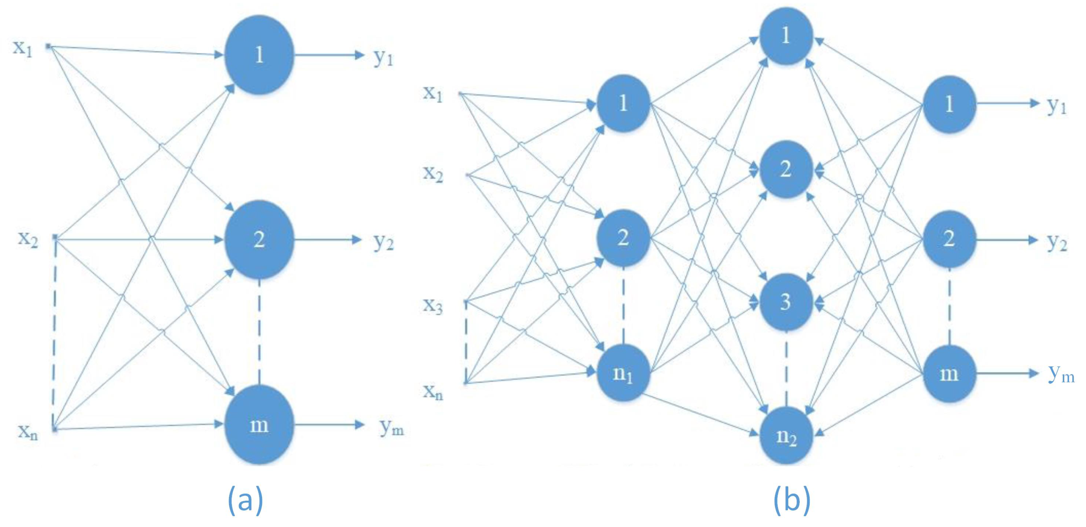
3.1. Fully Connected Neural Networks

The architecture of a Fully Connected Neural Network defines how neurons are organized and interconnected inside a network. Training a particular architecture involves several steps that aim to adjust the weights and thresholds of neurons.
A neural network is generally composed of three parts, which are referred as layers. These are:
  • The input layer. It receives information, signals, features, or measurements made in the external environment. Network inputs are usually set to maximum values. As a result of the normalization stage, the numerical accuracy of the network’s mathematical operations increases.
  • The hidden, intermediate, or invisible layers. These layers are composed of neurons that are responsible for extracting the patterns associated with the analyzed process. Most of the internal processing of the neural network takes place at the level of these layers. There may be one or more hidden layers in a network.
  • The output layer. This layer is responsible for producing and presenting the network’s final outputs, which were obtained after the processing performed by the previous layers.
The fundamental component of a Fully Connected Neural Network is the perceptron [37]. The perceptron is an element that has a certain number of inputs, x i , i = 1 N , and it calculates the weighted sum of these inputs. For each input i, the weight β i can take one of the values { 1 , 1 } . Eventually, this sum is compared with a threshold, in order to obtain the output y, according to Equation (1).
y = 1 if i = 1 N w i · x i θ 0 if i = 1 N w i · x i < θ
where w i represents the input weights and θ is the threshold.
The condition from Equation (1) is unintelligible. Accordingly, there can be made two modifications to simplify it. First, the sum can be write as a dot product, w · x = i w i x i where w and x are vectors whose components are the weights and inputs, respectively. The second change is to move the threshold to the other side of the inequality and replace it with the perceptron’s bias, b = t h r e s h o l d . The bias represents a measure of how easily the perceptron will output 1. Using the bias rather than the threshold, the perceptron rule can be rephrased as:
y = 1 if w · x + b 0 0 if w · x + b > 0
The perceptron is not a complete model of decisions. Instead, a complex network of perceptrons can make better decisions. For this reason, Fully Connected networks are also known in the literature as Multi Layer Perceptrons (MLP) networks.
Their goal is to approximate a function f, as defined in Equation (3). The network learns the value of the parameter θ , which leads to the best approximation of the function.
y = f ( x ; θ )
Figure 1 shows the two types of Fully Connected networks: single-layer network and multilayer network. There are situations in which neural networks do not have all the connections. Lack of a connection is equivalent to zero weight.
Concerning single-layer networks, it can be seen that the number of outputs of the network coincides with the number of neurons. This type of network is generally used in model classification and linear filtering problems. Unlike single-layer networks, multilayer networks have more hidden neural layers. They are used in more complex issues, such as system identification and optimization. A multilayer network can be seen as a cascade of multiple single-layer networks.
The level of complexity increases with the number of layers that are used. In 1989, the theorem of universal approximation appeared, which states that there is a neural network that is large enough to achieve any desired degree of accuracy. The theorem, on the other hand, does not specify how extensive the network might be. The one who designs such a network must reach a compromise between the network’s complexity and accuracy offered.
In order to design a model, it is necessary to select a cost function, which depends on the weight values. Mean Squared Error (Equation (4)) is one of the most often used cost functions.
C ( w , b ) = 1 2 n x y ( x ) a 2
where w represents the weights in the network, b is the bias, n is the number of inputs involved, and the vector a represents the vector of the outputs when the vector x is at the input of the network. Minimizing this cost function is the purpose of any neural network.

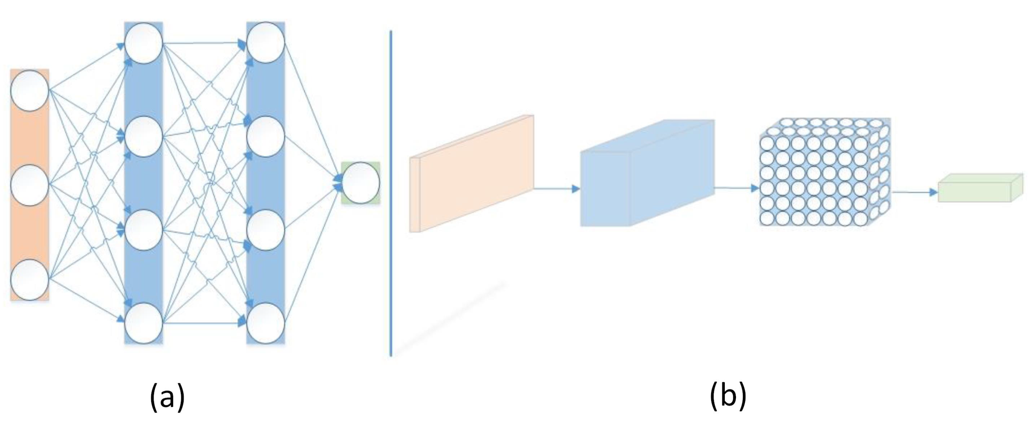
3.2. Convolutional Neural Networks

A CNN receives at the input an image, attributes importance to several objects within the image, and differentiates one from the other. CNN’s are composed of several layers of neurons that have different weights. The first layer of neurons receives the input data, while the performances that are offered by the network and the accuracy of the outputs are measured by a loss function (e.g., SVM, SoftMax) that is applied to the last neural layer.
The difference between a CNN and the Fully Connected networks relies in terms of input data, i.e., CNN relies on the assumption that the input data are an image. This assumption leads to specific changes in network architecture. Regarding the Fully Connected networks, the neurons are placed in two-dimensional layouts. Unlike this type of neural networks, the layers of a CNN are developed from neurons arranged in three-dimensional layouts. This essential difference can also be observed in Figure 2.
Generally, the CNN architecture contains the following types of layers:
  • Input layer. At this layer’s level, the pixel values from an image of various widths and heights are stored, using three color channels (R—Red, G—Green, B—Blue).
  • Convolution layer. It calculates the output of neurons that are connected to the input regions. The third dimension of the output changes depending on the number of filters (kernels) used in the convolution operation.
  • RELU layer. This layer applies an input data activation function, such as max ( 0 , x ) , with the threshold 0. The operations that take place at this layer do not change the size of the input data.
  • Pooling layer. It performs the subsampling operation along the spatial dimensions (width and height, respectively).
  • Fully Connected (FC) layer. This layer calculates the results for each class. Unlike all other layers, the neurons in this layer are connected to all of the previous layers’ neurons.
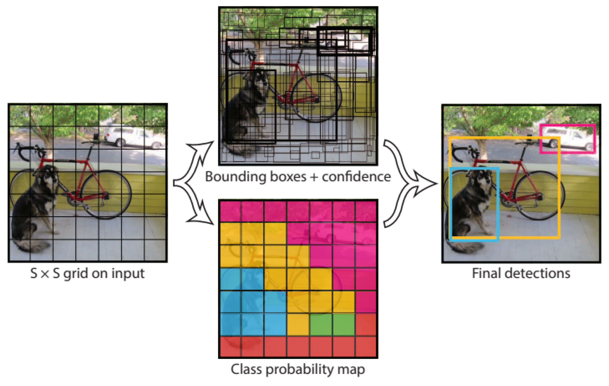
In this way, the CNN network transforms the original image, from the pixel values to all classes’ final probabilities. In image processing, these neural networks are predominantly used, because they allow for the use of information from the three image channels in order to extract essential characteristics of the images, which leads to high efficiency in terms of video processing.
Subsequently, Region-based Convolutional Neural Networks (R-CNN) [38] were implemented, which involve two stages: identifying regions of interest (RoI) in the image containing various objects and independently extracting CNN features from each region. Several versions of these networks were developed, which aimed to improve the performance in terms of both the processing time and method accuracy [39,40].

3.3. YOLO Model

In this paper, we use the YOLOv3 model [10], which is the last version of the original YOLO detection system [8]. There was also implemented YOLOv2 [41], an improved algorithm based on a smaller CNN, with fewer convolutional layers. However, although this network, called Darknet-19, has few layers, the running time and computational costs are comparable to those of the Darknet-53 neural network. Furthermore, the accuracy of the detection increases when using the third YOLO model.
The YOLO model is a general object detection system, which is more efficient and faster than the other existing methods. As the name suggests, a single network predicts both the location of objects and the probabilities directly from the original image, which makes it more suitable for applications for which real-time running represents a priority.
It treats object recognition as a unified regression problem instead of R-CNN, which are learned in order to perform classification. Additionally, YOLO sees the entire image during the training phase, which leads to better background recognition.
The YOLO model has several advantages when compared to other existing methods. Firstly, it is a faster system, since it treats the detection as a regression problem. Second, this model uses the entire input image when it performs final detection.
Unlike other techniques that use regions of interest, YOLO uses the full image in both the training and testing stages. The network uses the features of the entire image in order to predict each bounding box. Furthermore, all of the bounding boxes corresponding to all classes are predicted at the same time.
In Figure 3, the entire YOLO model is presented. The system divides the input image into S × S cells. The cell that is responsible for detecting an object is the cell located in the center of that object. Further, each cell predicts B bounding boxes and confidence scores for each bounding box. These scores reflect the system’s certainty that a bounding box contains an object and how accurate the prediction is.
For each predicted bounding box, the system generates five values:
  • (x, y), which represent the coordinates of the center of the bounding box;
  • (w, h), which represent the dimensions: the weight, and respectively, the height of the bounding box; and,
  • the prediction’s confidence, representing the Intersection Over Union (IOU) ratio between the predicted and the real bounding box.
Each cell also predicts C conditional probabilities, P r ( C l a s s i | O b j e c t ) , which depend on an object’s existence in that cell. The number of probabilities is the same as the number of classes. Only one set of such probabilities will be predicted, regardless of the number of existing framing rectangles. In the testing phase, it will obtain:
P r ( C l a s s i | O b j e c t ) · P r ( O b j e c t ) · I O U p r e d r e a l = P r ( C l a s s i ) · I O U p r e d r e a l
Equation (5) defines the confidence that represents the product between the probability of an object’s existence and the IOU size (calculated for the predicted and the real rectangle). If there is no object, then the confidence value is 0. This represents both the probability that a particular class of objects exists in the predicted framing rectangle and the accuracy with which it frames an object.
In the end, an image will contain S × S × B bounding boxes. Each bounding box corresponds to four predictions of the location, one confidence score, and C conditional probabilities, where C represents the number of classes. This leads to an amount of
N = S · S · ( 5 · B + C )
predicted values for a single image.

3.3.1. Darknet Architecture

Darknet neural network has multiple convolutional layers. Figure 4 presents the architecture of this network. The last two layers are fully connected. While the first layers extract the input image features, the last two layers predict the probabilities and output coordinates. The weight and the height of the predicted bounding boxes are normalized to the input image’s size. Therefore, the output values will be in the range [0, 1].
The YOLO model is trained in order to minimize the sum-squared error. Two scaling parameters are also introduced to control the loss function. This function is computed while using the equation:
L = λ c o o r d i = 0 s 2 j = 0 B 1 i j o b j [ ( x i x ^ i ) 2 + ( y i y ^ i ) 2 + ( w i w ^ i ) 2 + ( h i h ^ i ) 2 ] + i = 0 s 2 j = 0 B 1 i j o b j ( C i C ^ i ) 2 + λ n o o b j i = 0 s 2 j = 0 B 1 i j o b j ( C i C ^ i ) 2 + i = 0 s 2 1 i o b j c ϵ c l a s e [ p i ( c ) p ^ i ( c ) ] 2
where:
  • 1 i o b j 
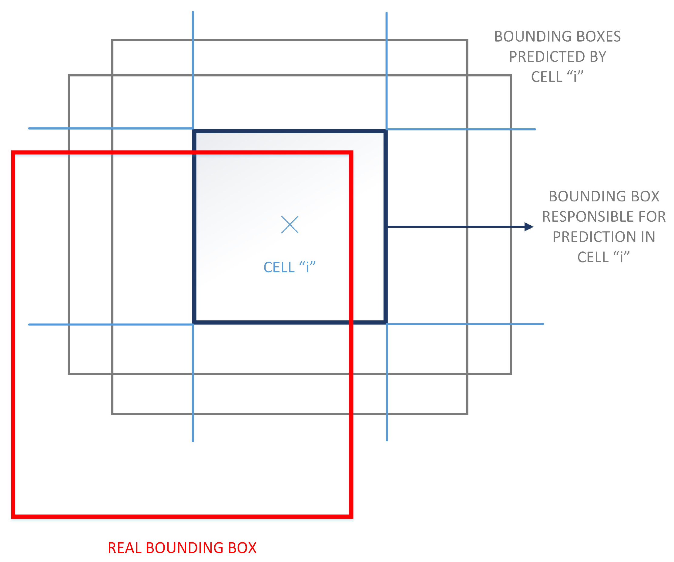
indicates if there is an object in cell i;
  • 1 i j o b j refers to the bounding box j in cell i, which is responsible for the prediction. This is the bounding box with the highest IOU relatively to the real bounding box (described in Figure 5).
  • C i represents the confidence score of the responsible predictor, from cell i;
  • C ^ i represents the predicted confidence score;
  • P i ( c ) defines the conditional probability that the cell i contains an object from class c; and,
  • λ c o o r d represents the scaling parameter that leads to the increasing of the loss function according to the coordinates’ predictions of bounding boxes. YOLO model uses the parameter
λ c o o r d = 5
  • λ n o o b j represents the scaling parameter that leads to the decreasing of the loss function, according to the predictions for the confidence score of the bounding boxes that do not contain objects. This system uses the scaling parameter
    λ n o o b j = 0.5
According to Equation (7), the classification errors only appear when there is an object in cell i, while, otherwise, 1 i o b j = 0 . Furthermore, the coordinates error only intervenes when it comes to the responsible predictor. For all the others predictors, 1 i j o b j = 0 .
Because to the improvements, the YOLO model has several advantages when compared to other classification-based systems. First of all, it knows the image’s global context, because it looks at the whole image, not only in the image regions.
Furthermore, it makes predictions after a single network evaluation, unlike the R-CNN network, which requires thousands of evaluations for a single image. This also leads to the second advantage. The YOLO model is high-speed. It is 1000 times faster than than the R-CNN network, and it is 100 times faster than the Fast R-CNN network [8].

3.3.2. YOLO Third Version

The newest version of the YOLO model trains a new and deeper neural network with more convolutional layers, while it also leads to more accurate detections. Although the number of layers in the network increases, it remains almost as fast as the previous versions [10].
Darknet-53 neural network predicts three bounding boxes, in order to frame the objects of different dimensions. For each bounding box, five values are predicted, i.e., t x , t y , t w , t h , and t o . When considering a cell displaced by ( c x , c y ) from the upper left corner of the image and a bounding box with dimensions p w and p h , respectively, the predictions will be computed using Equations (10)–(14). Additionally, Figure 6 describes the location prediction and related parameters.
b x = σ ( t x ) + c x
b y = σ ( t y ) + c y
b w = p w · e t w
b h = p h · e t h
P r ( o b j e c t ) · I O U ( b , o b j e c t ) = σ ( t 0 )
Additionally, the system predicts all of the classes that a bounding box may contain, while using a multiple label classification. In the end, the network will predict a number of N = 3 · ( 5 + C ) values. This model has 80 classes, which will lead to 255 parameters at the end of the network. The number of values also affects the number of layers from the last convolutional layer, which must always be equal to the neural network’s number of outputs.
One of the problems regarding the older versions of the YOLO model was the detection of small objects. The YOLOv3 model improves this detection. This model locates small objects with high accuracy due to the use of multi-scale predictions, which leads to a better and more efficient detection system.

4. Proposed Method

The primary purpose of this paper is to implement an efficient re-identification system. We started with the general detection system, YOLO, as described in the previous section. We aim to design a CNN that generates the feature vectors of each existing person in the databases, taking into account two essential elements. Firstly, the distance between the feature vectors that belong to persons with the same ID must be as small as possible, so that inner-class variation is not too significant. Furthermore, the feature vectors of different people must be as different as possible in order to separate the clusters.
Initially, we intended to implement a network with a small number of convolutional layers and generate a feature vector with reduced dimension. We started by extracting various layers from the Darknet network. In order to choose those layers, we analyzed the feature maps that were generated while using the tool described in [42]. We also extracted the associate weights that were pretrained from the YOLO model and we continue training it with our dataset. We tried different losses, like quadruplet loss [33] or center loss [43]. However, none of the versions led to the convergence of the re-identification system.
Further, we tended to use a deeper neural network and then divide the problem of re-identification into two stages. First, we aim to achieve a recognition system [2] of people from the database, followed by a stage of generalization, which will turn the recognition into a broader problem, i.e., person re-identification.

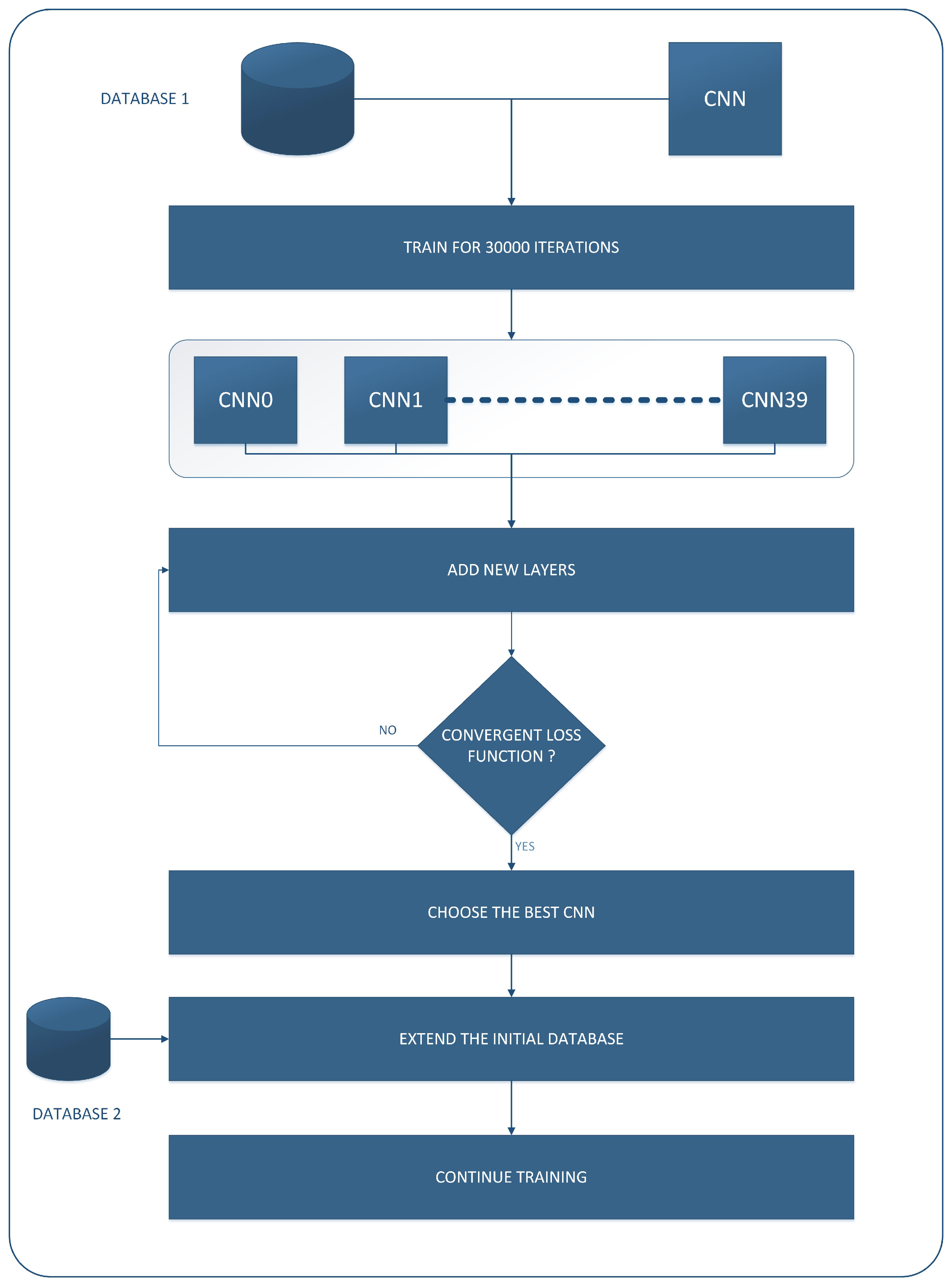
4.1. Algorithm Description

The first step of the algorithm is to train the CNN in order to obtain an accurate classifier, as can be seen in the diagram from Figure 7. The first stage has the primary purpose of initializing the weights used in convolutional layers. The network is initially trained on a small database for 30,000 iterations.
Further, from the obtained network, we generate more network architectures. Each network is trained using the same database, while, during the training phase, each network that does not converge is eliminated.
Further, the remaining networks are modified in order to be suitable for the re-identification problem. For this purpose, we added several layers at the end of each CNN and continue to train them on a bigger database. We aimed to obtain as many architectures as possible. We tried to change the last layers several times for each network if it does not converge. Finally, after training all of the remaining networks (using several layers), we choose the CNN that leads to the best results regarding re-identification. In the end, we take the best network and continue to train it using a vast database with a large number of subjects.
All of the presented stages and obtained results are described later in this paper.

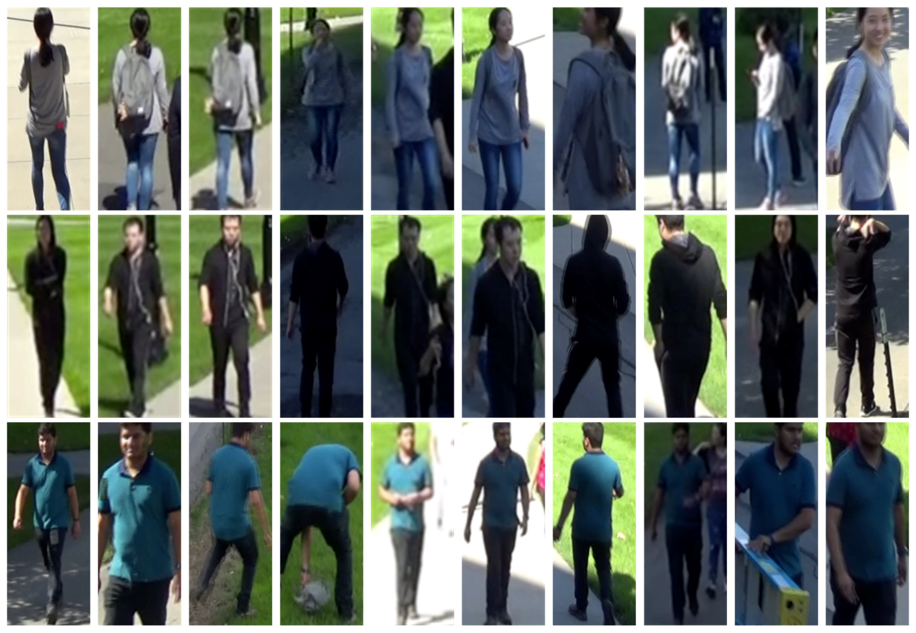
4.2. Image Databases

In this paper, we used two image databases, i.e., one for the training phase and one for testing our proposed method. This section presents both of the databases.
Firstly, we target an image dataset with several identities regarding the training phase, but we also need images with only one person. This is the reason why we have chosen the RPIField database [18] in this stage. This database contains 112 known identities. For each identity from the database, there are 12 camera views available, which is an essential feature of this dataset. Besides the known identities, which appear on each camera, there are also several unknown pedestrians.
The naming of each folder and each image is very helpful, being easier to generate a set of triplets when there is a well-known rule. The rule for naming the folder is personID_appearance, while the rule for naming an image from folders is CameraNO_FrameNO.png. For each image from the database, there is an associated .txt file. This file provides the location of the person within the image as well as the label.
Before training the neural network while using the RPIField database, we went through a database processing step. We propose only keeping the clean images to not introduce the wrong information through the network. Thus, the processing step involves several actions:
  • eliminating all the images that contain two or more persons;
  • eliminating all the images in which a person is partially hidden by other object, or is not fully captured on camera; and,
  • we eliminate all of the blurred images and the out of focus ones, in order to remove noise from database.
After this step, we only kept the clear images, which completely capture a person. In Figure 8, some samples that are extracted from the RPIField database are presented.
From this database, we initially used only 900 images that belonged to 30 people. Those images were randomly chosen from the clean database. After that, we formed the triplets that were used in the second phase of training from this small subset of images. Later in the training stage, we expanded the database to 60 images per subject, forming 1800 images.
Regarding the testing stage, we first tested our method on a subset of images that were extracted from the same database. Most importantly, we tested it on a completely different database, i.e., PRW-v16.04.20 [19]. This image database contains frames that are captured with six different cameras. Each frame has several persons, which makes the re-identification process more difficult. The images represent crowded places and, inevitably, there are occlusions of people, thus making re-identification impossible in certain situations.
We used this second database in order to test our system’s performances in a different situation, i.e., in a more general scenario. Figure 9 captures several frames that were extracted from this database.

4.3. First Training Phase

The first phase of the proposed method is to solve the recognition problem. As a starting point, we chose a CNN that consists of the first 80 layers extracted from the Darknet-53 neural network and the associated weights. The purpose was to start from a trained set of weights and avoid randomizing them. In this way, we increase the probability that the network will converge and we also try to avoid the idea of exploding gradients.
In this training stage, we consider a simple classification problem [10]. In order to do that, in the last layer, we use the logistic function for activation. This function is computed according to Equation (15). Further, for the prediction of classes, the binary cross-entropy loss is used, which is computed according to Equation (16).
f ( x ) = 1 1 + e x
L o s s = 1 N i = 1 N y i · log y ^ i + ( 1 y i ) · log ( 1 y ^ i ) ,
where N is the output size, y ^ i represents the i-th scalar from the output, and y i is the corresponding target value.
In this stage, we aim to perform the recognition of 30 classes. Accordingly, we chose from the database 30 subjects and 30 images for each subject, thus obtaining a small training database with 900 images in total.

4.4. Second Training Phase

During the second phase, we focus on converting the recognition problem into a more general one, i.e., person re-identification. To do so, we eliminate the last convolutional layer and classification layer, and we replaced them with other layers.
We only added convolutional layers and fully connected (FC) layers. The FC layers’ purpose was to reduce the feature vector’s size until we reached the desired dimension. At the end of the network, we designed a brand new layer, which implements the triplet loss function inside the YOLO framework. This layer optimizes the network in order to minimize the triplet loss in a more general way. We excluded the concept of classes, which gives us a greater degree of freedom. In this way, we are able to re-identify many people without considering their belonging to a particular class.
Unlike the initial classification while using the YOLO model, by adding the layer that we have designed, the network architecture becomes invariant to the number of classes that we train. Another advantage of the proposed method is the minimum volume of computational requirements and the shorter time that is required to train each network. This is a consequence of the reduced number of additional layers added and trained, with the rest of the layers from the first phase of the algorithm being frozen.
Starting from the Darknet network’s original parameters used in the first stage, we obtained 40 different variations. The most important parameters with the most significant impact on the network convergence are the learning rate and momentum. For these reasons, we varied both of the parameters according to Equations (17) and (18).
L R { 10 3 , 10 4 , 10 5 , 10 6 }
m o m e n t u m { 0.90 , 0.91 , 0.92 , , 0.99 }
The main goal was to obtain more network architectures in order to determine which one leads to the fastest convergence and most accurate re-identification.

4.4.1. Proposed Neural Network Architecture

The proposed architecture is not very different from the one used in the first phase. We have excluded the last two layers. The last convolutional layer was used in order to obtain (at the end of the network) the specific number of values that are described in Section 3. The number of filters in this layer varies with the number of classes. In our case, because we started with 30 classes in the previous phase, we had
N = 3 · ( 5 + 30 ) = 105
filters.
We excluded both the classification and last convolutional layer, because we do not want to further treat the re-identification as a problem of recognition. Instead, we added the layers that are described in Table 2 at the end of the neural network. As can be seen, we did not add any additional layers because we tried to keep at a minimum the computational power and the required additional memory. We froze all of the previous layers during this second training stage, aiming to train only the new layers.
Regarding the last layer, the re-identification one represents one of the novelties introduced by the proposed method. It implements several types of triplet losses in order to make the YOLO model suitable for person re-identification.

4.4.2. Triplet Loss

Triplet loss is a loss function that is often used in machine learning methods [44,45]. This function provides the idea of similarity, respectively, dissimilarity of images from a database. If the number of classes is considered to be known before training in the classification methods, using triplet loss is no longer necessary. Thus, the training phase does not have to be resumed every time that a new class is added.
In this way, the re-identification is seen as a problem of similarity, not of recognition. The main difference is that, for each input image, two more images are needed, thus forming a triplet. The three images from the triplet represent:
  • Anchor image. This is the image from the batch, which will pass through the network.
  • Positive image. It is an image similar to the anchor image (practically, from the same class).
  • Negative image. This must be dissimilar to the anchor image, belonging to another class.
Mathematically, triplet loss is computed while using Equation (20), being practically an Euclidean distance [44].
L ( A , P , N ) = [ D ( A , P ) D ( A , N ) + α ] +
[ D ( A , P ) D ( A , N ) + α ] + = m a x ( 0 , D ( A , P ) D ( A , N ) + α ) ,
where D ( x , y ) represents a distance between two learned feature vectors, x and y. As distance, one of the distances presented in Table 3 can be used. The second parameter used in triplet loss (i.e., the margin α ) represents the distance between two clusters. The purpose of this loss function is to ensure that for each anchor A, its features representation is closer to the positive image’s representation than that of the negative image, by at least α .
Those triplets can be chosen in many different ways, when considering the extent to which the anchor and the positive image are similar, or even to which the negative image differs from the anchor. One of the most common ways to choose triplets is the so-called hard negative triplets. In this case, we choose, for every anchor, the most similar negative image, according to the condition presented in Equation (22). In the worst-case scenario, the similarity between the anchor and positive image will be smaller than the similarity between the anchor and negative image.
Another type of triplets is the semihard negatives triplets. In this case, according to Equation (24), we have to choose for every anchor, the negatives sample that is the most similar with the anchor, but also less similar than the corresponding positive image. Regarding the third type of triplets (i.e., the moderate positives) they are chosen based on both the conditions from Equations (22) and (23).
D ( A , N ) = min i D ( A , N i )
D ( A , P ) = max i D ( A , P i )
D ( A , P ) D ( A , N i ) < D ( A , P ) + α
In order to use triplet loss in an optimization problem, a cost function can be obtained, which represents the sum of all the losses:
L t r i p l e t = A , P , N [ D ( A , P ) D ( A , N ) + α ] +
For this cost function to work, the network must be trained long enough until it passes through all of the pairs ( A , P ) , so that all of the images belonging to the same person are associated with each other. Eventually, all of the appearances of the same person will form a single cluster.

4.4.3. Re-Identification Layer

The proposed method’s novelty is the new layer that we implemented and included in the YOLO system. The re-identification layer is based on deep metric embedding learning. We use the triplet loss as a metric function. In this second phase, the neural network is trained in order to minimize the cost function that is described in Equation (25).
Mathematically, the re-identification layer uses (as metric distance) the l2-norm of a vector from Equation (26). Further, the algorithm requires several vector computations, which are described in Equations (26)–(30).
X 2 2 = i = 1 N x i 2
X 1 = i = 1 N | x i |
X Y = [ x 1 y 1 , , x N y N ]
X + Y = [ x 1 + y 1 , , x N + y N ]
α X = [ α x 1 , , α x N ]
When the neural network architecture is designed, the developer must provide the network with all of the parameters that it needs. In the case of the re-identification layer, the necessary parameters are:
  • margin. This parameter is used in the computation of the triplet loss, according to Equation (20). If not provided, this parameter has the default value 0.
  • type of triplets. Three types of triplets can be used in our algorithm: hard triplets, semihard triplets, and moderate positives triplets. Those three methods are described in Table 4. If not provided, this parameter will take the default value, i.e., hard triplets.
  • number of samples. This parameter is used only when it comes to moderate positives triplets. In this case, the number of positive, respectively, negative samples are different from the number of batches.

5. Experimental Results

This section will describe the testing steps and the methods used to test our proposed method’s performance after each training phase.

5.1. Testing Algorithm

In order to test the performance of the proposed method and be able to monitor the evolution of this system, it was necessary to design a test environment. At the end of each training stage, it is necessary to test the networks and the weights that were obtained to identify the best variants.
The testing stage involves passing each image from the test database through the CNN, thus obtaining the feature vectors. The ultimate goal is to compare each feature vector with all of the other vectors that belong to the previous images, and finally associate people based on the similarity between the vectors.
For running such a system, storing a remarkably large number of feature vectors is necessary. The number of vectors is equivalent to the number of occurrences of all persons in the test database. There are millions of such occurrences in a real scenario, which leads to much-needed storage space. It was necessary to store the features vectors in a database for operating the system on a wide range of real-life scenarios.
The feature vectors are generated once a neural network receives an image at the input. These are then stored in the database. Finally, the vector with the most significant similarity is sought in order to achieve the association. In order to test the re-identification method, storing five parameters in the database for each occurrence was required:
  • ID. This column is generated automatically and also incrementally. It represents a sequence of unique and consecutive numbers, being present in any database.
  • LABEL. This value is, in fact, an Universally Unique Identifiers (UUID). It is a 128 bits identifier, which consists of a total of 32 hexadecimal digits. Each time the system generates a new label, it considers that a feature vector belonging to a new person is being introduced in the database. If the system connects with an existing person in the database, the associated label is copied and assigned to the newly entered person.
  • TRUE_LABEL. This column represents the true identity of a person. The value is extracted from the .txt files that accompany the test images. It must be provided to the system in the testing stage.
  • NORM. This value represents the l2-norm of the feature vector and it is computed based on Equation (26).
  • FEATURES. This column stores the feature vector. This vector represents the output generated by the neural network. It is an 128-dimensional vector, based on which we finally made the association between the persons from the database.
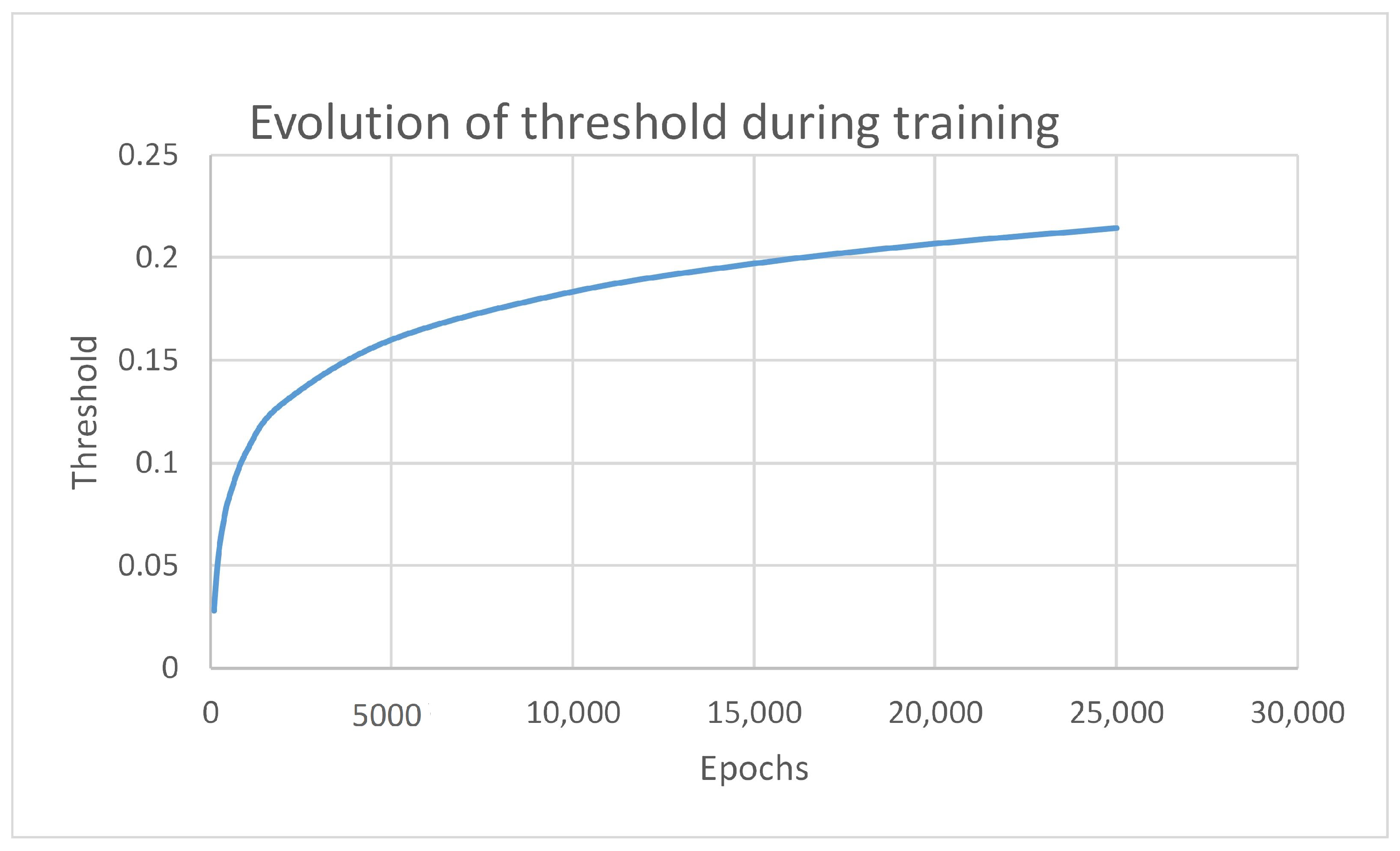
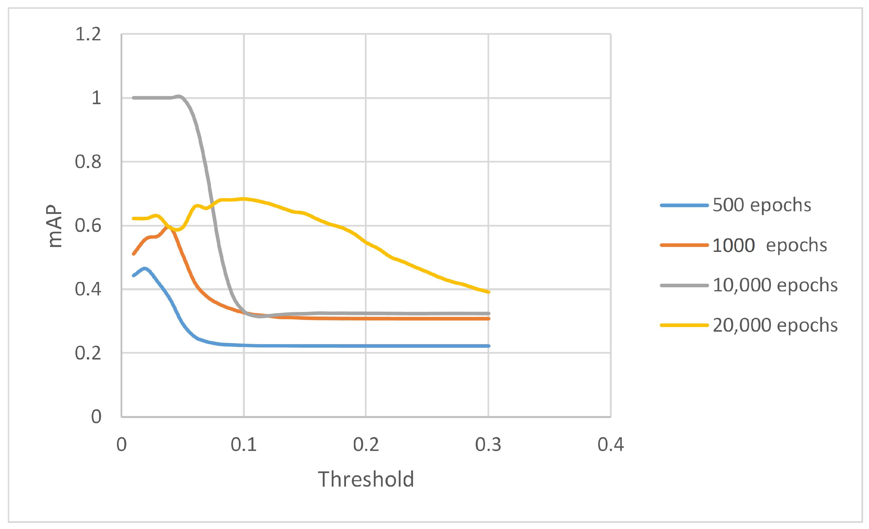
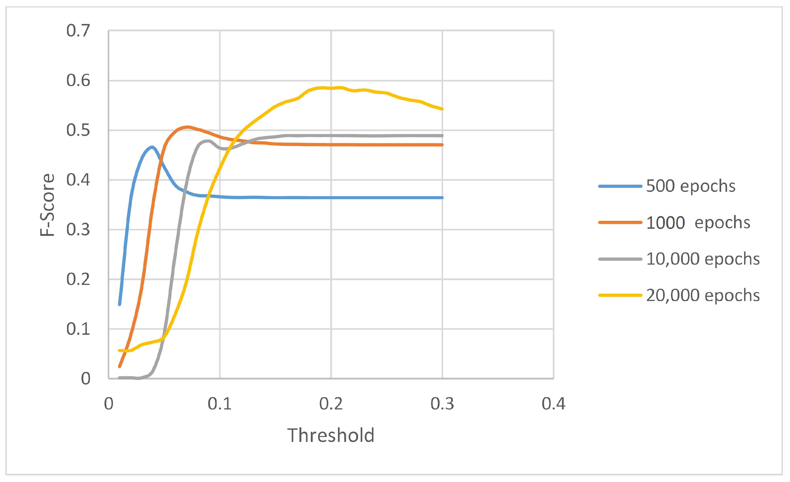
In Table 5, the algorithm according to which the database realizes the association between the feature vectors is described. Mathematically, there were relatively basics concept used, such as L1-norm, L2-norm, ascending order, and selections.
Knowing the minimum distance between the new feature vector and all of the other vectors from the database, we will further compare it with a previously set threshold. If the minimum distance is smaller than the threshold, we consider the two vectors to be similar and the system decides that the new person belongs to the same class with the most similar one. On the other side, if the minimum distance is greater than the threshold, then the system decides that there is no sufficiently similar vector in the database, and the new person is considered to be part of a new class, thus a new label is assigned. The threshold represents one of the main parameters of our proposed method. We used a wide range of thresholds (in all the designed tests) to find its optimal value.

5.2. Results

In order to observe how the CNN evolves, we created a series of scenarios, closely following these networks’ functioning. This helped us to intervene when the networks no longer converged, or the situation of gradients exploding appeared.
During the first phase of training, we trained the neural network on 30 classes, with a database of 900 images. Figure 8 presents some of the images used in this phase. This first step is only a classification one, in order to obtain the initial weights to start training in the following stage.
Table 6 presents the first results that were obtained after training all of the 40 variations of neural networks for several epochs. All of the tests executed in this first scenario are performed in some extreme and challenging conditions. While we trained our initial network on a particular distribution, using frames from RPIField database, we changed all of the conditions in this testing phase. We wanted to see how this system behaves, in a completely new environment, in which it was not trained at all. We aimed to obtain a system as general as possible, which does not only work on a trained database or in similar conditions. That is the reason why we have chosen the second database, PRW-v16.04.20 [19]. This database presents a real-life scenario, capturing a crowded location with many people and objects that partially overlap.
We compute both the mean Average Precision (mAP) and the F-score in order to determine the performance of our method. While mAP considers only positive detections (true positives and false positives), F-score is calculated based on mAP and recall. Accordingly, it also takes the false negative detections into account. The F-score represents the harmonic average of the two scores, being calculated with Equation (31). This score is used in deep learning to measure the accuracy of a model on a given database.
F score = 2 · mAP · recall mAP + recall
The tests that are described in Table 6 were realized on a dataset formed by 2800 images. From 2800 images, there were 6276 appearances of persons belonging to 621 classes. The main reason for this first test was to identify the best values for the learning rate and momentum.
Of the 40 neural networks trained and tested, some did not converge. For this reason, only 13 neural networks are shown in Table 6. These are the networks that have managed to converge and optimize the classification problem. In order to differentiate the networks, each received a unique ID. This is represented in the first column of the table.
While we followed the variation of the mAP and its comparison with other existing methods, the best model in terms of the total performance was chosen based on the F-score’s value. Following the first test results, it was concluded that the CNN with I D = 5 leads to the highest performance (as marked in Table 6). For this reason, the following tests are performed while using this CNN architecture: L R = 10 4 , m o m e n t u m = 0.91 , and b a t c h _ s i z e = 64 .
Furthermore, we focused on training this particular network over a more extended period in order to see how it behaves. Figure 10 shows the obtained results. After we trained our proposed model, we tested it using Rank1, Rank5, Rank10, and Rank20. Our proposed method achieves an Rank-20 accuracy of up to 0.72.
As the rank increases, so does the performance of the model. However, it also increases both the computational complexity and running time. Thus, Rank-5 offers a good compromise.
For each test presented, we computed the results while using different thresholds. We varied the threshold in the range ( 0 , 1 ] , using a step Δ = 0.01 . Figure 11 shows the evolution of the threshold when training the proposed CNN. This parameter represents the minimum distance from which the algorithm separates two classes. Thus, the distance between two embeddings belonging to different classes is reduced. Once the threshold is low, both the intra-class and inter-class variations are reduced, and the method does not efficiently separate different classes.
Once the threshold increases, the inter-class variation increases, and the neural network is more accurately learning the differences between the characteristics of each class. In the proposed method, we trained the network while using triplet loss optimization, with a value margin of 0.2.
Ideally, the threshold will tend toward the margin value. In our case, the threshold tends to 0.23 as the training progresses, as can be seen in Figure 11.
Next, in Figure 12 and Figure 13, the system’s evolution is presented in terms of the mAP and F-score. The evolution of the F-score is closely related to one of the thresholds. As the number of training epochs increases, the maximum value of the score also increases. Furthermore, the maximum point of the function changes and it tends to the threshold’s optimal value (0.2).
We focused on obtaining a general system re-identification, and so this is why all of these tests were realized across data distributions. While the whole training phase was performed on a small part of the RPIField database, the testing was performed entirely on a completely different database. Furthermore, the tests were realized in some crowded places, with several occlusions of people. This leads to the hiding of some features, with the neural network not receiving the complete information that it needs.
In order to compare the proposed method’s accuracy with other existing methods, we chose another method that is based on deep metric learning. According to [34], the SphereReID method has led to better results than the other methods. For this reason, we trained the network proposed in [34] on the same database that was used in our method, for 25,000 epochs. Subsequently, we tested both variants on a dataset extracted from the PRW-v16.04.20 database. It can be observed from Figure 14 that our proposed method outperforms the second method in the scenario stated in this paper. Also, in terms of the time performances, our proposed method is more efficient, tending to a duration of 120 ms/identity as the number of examples stored in the database increases. It can be seen that our proposed method leads to a Rank-1 accuracy of almost 0.5.

6. Conclusions and Future Work

This paper has shown that a general-purpose DNN object detector, like the YOLO model, can address the person re-identification problem. The main goal was to implement a method that would achieve re-identification with the minimum requirements for computing and hardware resources.
Our proposed method treats the re-identification as a classification problem, while the second part generalizes it. In this way, we only added five new layers to be trained. The small number of supplementary layers leads to a high processing speed, reducing both the time and resources required. We aimed to design a system that runs in real-time and generates as few computational costs as possible, but it would lead to a high re-identification rate.
When considering all of these requirements, our proposed method manages to implement the first version of a general re-identification system. After testing a database utterly different from the one used in the learning stage, we obtained a Rank-1 re-identification rate of 50% and a Rank-20 of 72% (based on F-score function). This is a promising result in generalizing re-identification and achieving a robust and invariant system for variations of data distributions. Furthermore, besides recognizing a large number of people from an entirely new database, our algorithm is fast, providing the right balance between the speed, cost, and re-identification rate.
Regarding future work, we intend to implement an improved version of the system that will increase the re-identification rate, keeping speed, and additional costs to a minimum. We aim to obtain a fully automatic re-identification system, containing a stage of detection of persons before the stage of re-identification.
In conclusion, this paper demonstrates that it is possible to implement a re-identification system that runs on a wide range of real-life scenarios. It is possible to obtain a high re-identification rate on distribution without collecting large volumes of data from security systems or retrain the network while using a limited number of samples during the training stage. While, historically, person re-identification methods were dependent on a specific database, our paper shows that a system can still be usable on other distributions with minimal effort, even if the accuracy still needs some improvement.

Author Contributions

Conceptualization, R.-E.M. and S.C.; methodology, M.G.; software, R.-E.M. and M.C.; validation, C.P.; formal analysis, M.C. and S.C.; investigation, R.-E.M.; supervision, C.P. All authors have read and agreed to the published version of the manuscript.

Funding

This work was supported by grants of the Romanian Ministry of Education and Research, CNCS – UEFISCDI, project number: PN-III-P1-1.1-TE-2019-0420, project number: PN-III-P2-2.1-PTE-2019-0055, and project number PN-III-P2-2.1-PTE-2019-0570.

Conflicts of Interest

The authors declare no conflict of interest.

Abbreviations

The following abbreviations are used in this manuscript:
YOLOYou Only Look Once
DNNDeep Neural Network
CNNConvolutional Neural Network
FCFully Connected
MLPMulti Layer Perceptrons
R-CNNRegion based Convolutional Neural Network
RoIRegion of Interest
IOUIntersection Over Union
ORDBMSObject-Relational Database Management System
MVCCMulti-Version Concurrency Control
ODBCOpen Database Connectivity
TCPTransmission Control Protocol
IPInternet Protocol
UUIDUniversally Unique Identifiers
mAPmean Average Precision

References

  1. Arca, S.; Campadelli, P.; Lanzarotti, R. A face recognition system based on automatically determined facial fiducial points. Pattern Recognit. 2006, 39, 432–443. [Google Scholar] [CrossRef]
  2. Ghenescu, V.; Mihaescu, R.E.; Carata, S.V.; Ghenescu, M.T.; Barnoviciu, E.; Chindea, M. Face detection and recognition based on general purpose dnn object detector. In Proceedings of the 2018 International Symposium on Electronics and Telecommunications (ISETC), Timisoara, Romania, 8–9 November 2018; pp. 1–4. [Google Scholar]
  3. Lalonde, M.; Foucher, S.; Gagnon, L.; Pronovost, E.; Derenne, M.; Janelle, A. A system to automatically track humans and vehicles with a PTZ camera. In Visual Information Processing XVI; Ur Rahman, Z., Reichenbach, S.E., Neifeld, M.A., Eds.; International Society for Optics and Photonics, SPIE: Bellingham, WA, USA, 2007; Volume 6575, pp. 9–16. [Google Scholar] [CrossRef]
  4. Choi, W.; Pantofaru, C.; Savarese, S. A general framework for tracking multiple people from a moving camera. IEEE Trans. Pattern Anal. Mach. Intell. 2012, 35, 1577–1591. [Google Scholar] [CrossRef] [PubMed]
  5. Kim, C.; Lee, J.; Han, T.; Kim, Y.M. A hybrid framework combining background subtraction and deep neural networks for rapid person detection. J. Big Data 2018, 5, 22. [Google Scholar] [CrossRef]
  6. Gong, S.; Cristani, M.; Loy, C.C.; Hospedales, T.M. The re-identification challenge. In Person Re-Identification; Springer: Berlin/Heidelberg, Germany, 2014; pp. 1–20. [Google Scholar]
  7. Zheng, M.; Karanam, S.; Radke, R.J. Towards Automated Spatio-Temporal Trajectory Recovery in Wide-Area Camera Networks. IEEE Trans. Biom. Behav. Identity Sci. 2020. [Google Scholar] [CrossRef]
  8. Redmon, J.; Divvala, S.; Girshick, R.; Farhadi, A. You only look once: Unified, real-time object detection. In Proceedings of the IEEE Conference on Computer Vision and Pattern Recognition, Las Vegas, NV, USA, 27–30 June 2016; pp. 779–788. [Google Scholar]
  9. Redmon, J. Darknet: Open Source Neural Networks in C. pp. 2013–2016. Available online: http://pjreddie.com/darknet/ (accessed on 14 December 2020).
  10. Redmon, J.; Farhadi, A. YOLOv3: An Incremental Improvement. arXiv 2018, arXiv:1804.02767. [Google Scholar]
  11. Bedagkar-Gala, A.; Shah, S.K. A survey of approaches and trends in person re-identification. Image Vis. Comput. 2014, 32, 270–286. [Google Scholar] [CrossRef]
  12. Gray, D.; Brennan, S.; Tao, H. Evaluating appearance models for recognition, reacquisition, and tracking. In Proceedings of the IEEE International Workshop on Performance Evaluation for Tracking and Surveillance (Pets), Rio de Janeiro, Brazil, 14 October 2007; Citeseer: Princeton, NJ, USA, 2007; Volume 3, pp. 1–7. [Google Scholar]
  13. Li, W.; Wang, X. Locally aligned feature transforms across views. In Proceedings of the IEEE Conference on Computer Vision and Pattern Recognition, Portland, OR, USA, 23–28 June 2013; pp. 3594–3601. [Google Scholar]
  14. Li, W.; Zhao, R.; Xiao, T.; Wang, X. DeepReID: Deep filter pairing neural network for person re-identification. In Proceedings of the IEEE Conference on Computer Vision and Pattern Recognition, Columbus, OH, USA, 23–28 June 2014; pp. 152–159. [Google Scholar]
  15. Zheng, L.; Shen, L.; Tian, L.; Wang, S.; Wang, J.; Tian, Q. Scalable person re-identification: A benchmark. In Proceedings of the IEEE International Conference on Computer Vision, Santiago, Chile, 7–13 December 2015; pp. 1116–1124. [Google Scholar]
  16. Zheng, L.; Bie, Z.; Sun, Y.; Wang, J.; Su, C.; Wang, S.; Tian, Q. Mars: A video benchmark for large-scale person re-identification. In European Conference on Computer Vision; Springer: Berlin/Heidelberg, Germany, 2016; pp. 868–884. [Google Scholar]
  17. Ristani, E.; Solera, F.; Zou, R.; Cucchiara, R.; Tomasi, C. Performance measures and a data set for multi-target, multi-camera tracking. In European Conference on Computer Vision; Springer: Berlin/Heidelberg, Germany, 2016; pp. 17–35. [Google Scholar]
  18. Zheng, M.; Karanam, S.; Radke, R.J. RPIfield: A new dataset for temporally evaluating person re-identification. In Proceedings of the IEEE Conference on Computer Vision and Pattern Recognition Workshops, Salt Lake City, UT, USA, 18–22 June 2018; pp. 1893–1895. [Google Scholar]
  19. Zheng, L.; Zhang, H.; Sun, S.; Chandraker, M.; Yang, Y.; Tian, Q. Person Re-identification in the wild. In Proceedings of the IEEE Conference on Computer Vision and Pattern Recognition, Honolulu, HI, USA, 21–26 July 2017; pp. 1367–1376. [Google Scholar]
  20. Khan, F.M.; Brèmond, F. Multi-shot person re-identification using part appearance mixture. In Proceedings of the 2017 IEEE Winter Conference on Applications of Computer Vision (WACV), Santa Rosa, CA, USA, 24–31 March 2017; pp. 605–614. [Google Scholar]
  21. Ye, M.; Shen, J.; Lin, G.; Xiang, T.; Shao, L.; Hoi, S.C. Deep learning for person re-identification: A survey and outlook. arXiv 2020, arXiv:2001.04193. [Google Scholar]
  22. Gao, H.; Chen, S.; Zhang, Z. Parts semantic segmentation aware representation learning for person re-identification. Appl. Sci. 2019, 9, 1239. [Google Scholar] [CrossRef] [Green Version]
  23. Chen, B.; Zha, Y.; Min, W.; Yuan, Z. Person Re-identification Algorithm Based on Logistic Regression Loss Function. J. Phys. Conf. Ser. 2019, 1176, 032041. [Google Scholar] [CrossRef]
  24. Luo, Y.; Wong, Y.; Kankanhalli, M.; Zhao, Q. G -Softmax: Improving Intraclass Compactness and Interclass Separability of Features. IEEE Trans. Neural Networks Learn. Syst. 2019, 31, 685–699. [Google Scholar] [CrossRef] [PubMed]
  25. Shrestha, A.; Mahmood, A. Enhancing Siamese Networks Training with Importance Sampling. In Proceedings of the 11th International Conference on Agents and Artificial Intelligence (ICAART 2019), Prague, Czech Republic, 19–21 February 2019; pp. 610–615. Available online: https://www.scitepress.org/Papers/2019/73717/73717.pdf (accessed on 14 December 2020). [CrossRef]
  26. Liu, Z.; Qin, J.; Li, A.; Wang, Y.; Van Gool, L. Adversarial binary coding for efficient person re-identification. In Proceedings of the 2019 IEEE International Conference on Multimedia and Expo (ICME), Shanghai, China, 8–12 July 2019; pp. 700–705. [Google Scholar]
  27. Zhao, Y.; Jin, Z.; Qi, G.J.; Lu, H.; Hua, X.S. An Adversarial Approach to Hard Triplet Generation. In Proceedings of the European Conference on Computer Vision (ECCV), Munich, Germany, 8–14 September 2018; pp. 508–524. [Google Scholar]
  28. Zhang, Y.; Zhong, Q.; Ma, L.; Xie, D.; Pu, S. Learning incremental triplet margin for person re-identification. In Proceedings of the AAAI Conference on Artificial Intelligence, Honolulu, HI, USA, 27 January–1 February 2019; Volume 33, pp. 9243–9250. [Google Scholar]
  29. Shi, H.; Yang, Y.; Zhu, X.; Liao, S.; Lei, Z.; Zheng, W.; Li, S. Embedding Deep Metric for Person Re-identification: A Study Against Large Variations. In Computer Vision—ECCV 2016; Springer: Cham, Switzerland, 2016; Volume 9905, pp. 732–748. Available online: https://arxiv.org/pdf/1611.00137.pdf (accessed on 14 December 2020). [CrossRef]
  30. Manmatha, R.; Wu, C.Y.; Smola, A.; Krahenbuhl, P. Sampling Matters in Deep Embedding Learning. 2017; pp. 2859–2867. Available online: https://arxiv.org/pdf/1706.07567.pdf (accessed on 14 December 2020). [CrossRef] [Green Version]
  31. Suh, Y.; Wang, J.; Tang, S.; Mei, T.; Lee, K. Part-Aligned Bilinear Representations for Person Re-identification. arXiv 2018, arXiv:1804.07094. [Google Scholar]
  32. Ristani, E.; Tomasi, C. Features for Multi-Target Multi-Camera Tracking and Re-Identification. arXiv 2018, arXiv:1803.10859. [Google Scholar]
  33. Chen, W.; Chen, X.; Zhang, J.; Huang, K. Beyond Triplet Loss: A Deep Quadruplet Network for Person Re-identification. In Proceedings of the 2017 IEEE Conference on Computer Vision and Pattern Recognition (CVPR), Honolulu, HI, USA, 21–26 July 2017. [Google Scholar] [CrossRef] [Green Version]
  34. Fan, X.; Jiang, W.; Luo, H.; Fei, M. SphereReID: Deep Hypersphere Manifold Embedding for Person Re-Identification. J. Vis. Commun. Image Represent. 2019, 60. [Google Scholar] [CrossRef] [Green Version]
  35. Kumar, D.; Siva, P.; Marchwica, P.; Wong, A. Unsupervised Domain Adaptation in Person re-ID via k-Reciprocal Clustering and Large-Scale Heterogeneous Environment Synthesis. In Proceedings of the IEEE Winter Conference on Applications of Computer Vision, Snowmass Village, CO, USA, 2–5 March 2020; pp. 2645–2654. [Google Scholar]
  36. Alom, M.Z.; Taha, T.; Yakopcic, C.; Westberg, S.; Sidike, P.; Nasrin, M.; Hasan, M.; Essen, B.; Awwal, A.; Asari, V. A State-of-the-Art Survey on Deep Learning Theory and Architectures. Electronics 2019, 8, 292. [Google Scholar] [CrossRef] [Green Version]
  37. McCulloch, W.S.; Pitts, W. A logical calculus of the ideas immanent in nervous activity. Bull. Math. Biophys. 1943, 5, 115–133. [Google Scholar] [CrossRef]
  38. Girshick, R.; Donahue, J.; Darrell, T.; Malik, J. Rich Feature Hierarchies for Accurate Object Detection and Semantic Segmentation. In Proceedings of the IEEE Computer Society Conference on Computer Vision and Pattern Recognition, Columbus, OH, USA, 23–28 June 2014. [Google Scholar] [CrossRef] [Green Version]
  39. Girshick, R. Fast r-cnn. In Proceedings of the 2015 IEEE International Conference on Computer Vision (ICCV), Santiago, Chile, 7–13 December 2015. [Google Scholar] [CrossRef]
  40. Ren, S.; He, K.; Girshick, R.; Sun, J. Faster R-CNN: Towards Real-Time Object Detection with Region Proposal Networks. IEEE Trans. Pattern Anal. Mach. Intell. 2016, 39, 1137–1149. [Google Scholar] [CrossRef] [PubMed] [Green Version]
  41. Redmon, J.; Farhadi, A. YOLO9000: Better, Faster, Stronger. arXiv 2016, arXiv:1612.08242. [Google Scholar]
  42. Carata, S.; Mihaescu, R.; Barnoviciu, E.; Chindea, M.; Ghenescu, M.; Ghenescu, V. Complete Visualisation, Network Modeling and Training, Web Based Tool, for the Yolo Deep Neural Network Model in the Darknet Framework. In Proceedings of the 2019 IEEE 15th International Conference on Intelligent Computer Communication and Processing (ICCP), Cluj-Napoca, Romania, 5–7 September 2019; pp. 517–523. [Google Scholar]
  43. Wu, D.; Zheng, S.J.; Bao, W.Z.; Zhang, X.P.; Yuan, C.A.; Huang, D.S. A novel deep model with multi-loss and efficient training for person re-identification. Neurocomputing 2019, 324, 69–75. [Google Scholar] [CrossRef]
  44. Hermans, A.; Beyer, L.; Leibe, B. In defense of the triplet loss for person re-identification. arXiv 2017, arXiv:1703.07737. [Google Scholar]
  45. Cheng, D.; Gong, Y.; Zhou, S.; Wang, J.; Zheng, N. Person re-identification by multi-channel parts-based CNN with improved triplet loss function. In Proceedings of the IEEE Conference on Computer Vision and Pattern Recognition, Las Vegas, NV, USA, 27–30 June 2016; pp. 1335–1344. [Google Scholar]
Figure 1. Types of Fully Connected Networks. (a) Single Layer Network; (b) Multi Layer Network.
Algorithms 13 00343 g001
Figure 2. Neuron layouts in different types of neural networks. (a) Fully Connected Neural Network; (b) Convolutional Neural Network.
Algorithms 13 00343 g002
Figure 3. The You Only Look Once (YOLO) [8] model.
Algorithms 13 00343 g003
Figure 4. Darknet architecture.
Algorithms 13 00343 g004
Figure 5. Bounding box responsible for prediction.
Algorithms 13 00343 g005
Figure 6. Bounding boxes and location prediction.
Algorithms 13 00343 g006
Figure 7. Diagram of proposed algorithm.
Algorithms 13 00343 g007
Figure 8. Examples extracted from RPIField Database [18]. There are three subjects which are captured from different views, by different cameras—Subjects with IDs 1, 6, and 20, respectively.
Algorithms 13 00343 g008
Figure 9. Examples extracted from PRW-v16.04.20 Database [19]. There are three different cameras that are capturing frames with several persons. The conditions are incredibly different when compared to RPIField database.
Algorithms 13 00343 g009
Figure 10. Performance of our proposed method according to Rank.
Algorithms 13 00343 g010
Figure 11. Evolution of the proposed threshold during the training phase.
Algorithms 13 00343 g011
Figure 12. mAP evolution according to the threshold. This test was performed for several sets of weights.
Algorithms 13 00343 g012
Figure 13. F-score evolution according to the threshold. This test was performed for several sets of weights.
Algorithms 13 00343 g013
Figure 14. Comparison between the proposed method and another method based on deep metric embedding learning; (a) Comparison in terms of running time; (b) Comparison in terms of precision.
Algorithms 13 00343 g014
Table 1. Comparing existing re-ID databases.
DatabaseFramesID’sAnnotated BoxBoxes per IDCameras
VIPeR [12] 632126422
CUHK02 [13] 18167264410
CUHK03 [14] 136013,1649.710
Market-1501 [15] 150125,25919.96
MARS [16] 12611,067,516846.56
DukeMTMC-reID [17] 185236,44119.78
RPIField [18]601,581112601,5815371.212
PRW-v16.04.20 [19]11,81693234,30436.86
Table 2. Proposed Network Architecture—layers added in the second phase of training.
Type of LayerInput DimensionsNumber of FiltersSizeStrideOutput Dimensions
Convolutional52 × 52 × 1281283226 × 26 × 128
Convolutional26 × 26 × 128641126 × 26 × 64
Fully Connected26 × 26 × 64---1024
Dropout1024---1024
Fully Connected1024---128
Dropout128---128
Re-Identification128----
Table 3. Distance metrics that are used in triplet loss.
Distance MetricEquation
Euclidean Distance D ( x , y ) = ( x 1 y 1 ) 2 + ( x 2 y 2 ) 2 + + ( x i y i ) 2 + + ( x N y N ) 2
1—cosine similarity D ( x , y ) = 1 i = 1 N x i · y i i = 1 N x i 2 i = 1 N y i 2
Table 4. Types of triplets implemented in our proposed method.
Type of TripletsAlgorithm
Hard negativeInitialization:
Set network parameters:
n e t _ b a t c h = 64 , n e t _ o u t p u t s = 128 , m a r g i n = 0.2 , t r i p l e t s = H A R D
For i = 1 , 2 , , number of batches:
 For j = 1 , 2 , , number of negative samples:
  Compute D ( A i , N j ) based on (28) and (26)
 Find for A i the most similar negative sample N j using (22)
 Compute D ( A i , P ) based on (28) and (26)
 Compute the triplet loss L i = L ( A i , P , N j ) using (20)
Compute the cost function based on (25)
Semi-hard negativesInitialization:
Set network parameters:
n e t _ b a t c h = 64 , n e t _ o u t p u t s = 128 , m a r g i n = 0.2 , t r i p l e t s = S E M I H A R D
For i = 1 , 2 , , number of batches:
 Compute D ( A i , P ) based on (28) and (26)
 For j = 1 , 2 , , number of negative samples
  Compute D ( A i , N j ) based on (28) and (26)
  Choose all the triplets that correspond to (24)
 Compute the number of semi-hard negative triplets for A i
 For k = 1 , 2 , , n u m b e r o f s e m i h a r d t r i p l e t s
  Compute the triplet loss L k = L ( A i , P , N k ) according to (20)
 Compute the partial cost function C i based on (25)
Compute the cost function by summing all the partial functions.
Moderate PositivesInitialization:
Set network parameters:
n e t _ b a t c h = 64 , n e t _ o u t p u t s = 128 , m a r g i n = 0.2 , n e t _ s a m p l e s = 100 , t r i p l e t s = M O D E R A T E
For i = 1 , 2 , , number of batches:
 For j = 1 , 2 , , number of negative samples:
  Compute D ( A i , N j ) based on (28) and (26)
 Find for A i the most similar negative sample N j using (22)
 For k = 1 , 2 , , number of positive samples:
  Compute D ( A i , P k ) based on (28) and (26)
 Find for A i the most different positive sample P k using (23)
 Check if the first part of the condition from (24) is fulfilled for D ( A i , P k ) and D ( A i , N j )
 If the condition is met, compute the triplet loss L i = L ( A i , P K , N j ) using (20)
Compute the cost function based on (25)
Table 5. Algorithm designed for PostgreSQL.
Algorithm for Finding the Most Similar Feature Vector from the Database
Initialization:
Set parameters from PostgreSQL database:
m i n _ d i s t a n c e = F L O A T _ M A X , n u m b e r _ o f _ r o w s , n o r m _ m a x , n o r m _ m i n
Compute | f | , as being the L1-norm of new feature vector based on (27)
Sort vectors ascending, according to L1-norm
Select k = n u m b e r _ o f _ r o w s most similar feature vectors, according to L1-norm
for i = 1 , 2 , , k :
    Compute the distance D ( f , f i ) , based on (28) and (26)
Compute the distance as being the minimum distance between the new feature vector and the others k vectors,
based on (22).
Table 6. Preliminary Rank-5 results obtained for mean Average Precision (mAP) and F-score by modifying the values for learning rate and momentum. All of these tests were implemented on PRW-v16.04.20 database.
NETWORKLEARNINGMOMENTUMEPOCHS TRAINEDmAPF-Score
IDRATE
1 10 4 0.9010,0000.5401670.599489
20,0000.5267940.58512
30,0000.5655350.592613
3 10 6 0.9010,0000.3489330.37761
20,0000.2988210.460086
30,0000.3940280.501042
5 10 4 0.9110,0000.4822610.568995
20,0000.5357480.578173
30,0000.4877420.604684
6 10 5 0.9110,0000.3538560.485571
20,0000.4110610.504279
30,0000.50.577131
7 10 6 0.9110,0000.5333330.397199
20,0000.467910.464961
30,0000.5274030.479184
13 10 4 0.9310,0000.5775770.614993
20,0000.5513970.568058
30,0000.548310.587156
15 10 6 0.9310,0000.2701890.425431
20,0000.3243630.489367
30,0000.5360480.49375
19 10 6 0.9410,0000.2579720.41014
20,0000.3000790.461632
30,0000.2819920.43265
21 10 4 0.9510,0000.3150370.475352
20,0000.3290390.489486
30,0000.3765140.538335
22 10 5 0.9510,0000.4002240.473076
20,0000.5291530.56472
30,0000.49090.544563
25 10 4 0.9610,0000.4604020.585877
20,0000.4387330.571622
30,0000.4392950.5609
34 10 5 0.9810,0000.4804840.576851
20,0000.5702230.599062
30,0000.519230.545269
39 10 6 0.9910,0000.3117380.475305
20,0000.3727430.472351
30,0000.4281610.557936
batch_size = 64, image_height = 416, image_weight = 416, max_epochs = 30, 000, classes = 852, appearances = 6276, rank = 5.
Publisher’s Note: MDPI stays neutral with regard to jurisdictional claims in published maps and institutional affiliations.

