Approximation Algorithm for Shortest Path in Large Social Networks


Big Data Research Center, University of Electronic Science and Technology of China, Chengdu 610051, China
*
Author to whom correspondence should be addressed.
Algorithms 2020, 13(2), 36; https://0-doi-org.brum.beds.ac.uk/10.3390/a13020036
Submission received: 31 December 2019
/
Revised: 28 January 2020
/
Accepted: 31 January 2020
/
Published: 6 February 2020
Abstract
:Proposed algorithms for calculating the shortest paths such as Dijikstra and Flowd-Warshall’s algorithms are limited to small networks due to computational complexity and cost. We propose an efficient and a more accurate approximation algorithm that is applicable to large scale networks. Our algorithm iteratively constructs levels of hierarchical networks by a node condensing procedure to construct hierarchical graphs until threshold. The shortest paths between nodes in the original network are approximated by considering their corresponding shortest paths in the highest hierarchy. Experiments on real life data show that our algorithm records high efficiency and accuracy compared with other algorithms.
1. Introduction
The internet and its associated technologies have changed the way society conducts businesses, and the way that families and friends relate with each other. Social networking has become so popular such that users have drifted from the traditional physical media (the print and broadcasting media) to a more sophisticated social interaction. Computer scientists are looking into designing tools, models, and applications in diverse fields in internet application technologies [1] such as communication [2], recommendations, social marketing, terrorist threats [3], and key node mining [4]. Efficiently computing the shortest path between any two nodes in a network is one of the most important concerns of researchers since it has a great potential for mobilizing people [5]. Exact algorithms such as Dijkstra’s and Floyd-Warshall’s algorithms have not performed so well on large scale networks due to their high computational complexity. Even though these algorithms are so popular for their accuracy and applications, they cannot be efficiently applied to our current trend of large-scale datasets. We design an approximate algorithm to calculate the distances of the shortest paths in a modeled large-scale network. Chow [6] presented a heuristic algorithm for searching the shortest paths on a connected, undirected network. Chow’s algorithm relies on a heuristic function whose quality affects the efficiency and accuracy of estimation. Rattgan et al. [7] designed a network structure index (NSI) algorithm to estimate the shortest path in networks by storing data in a structure. Construction of the structure however consumes so much time and space. Tang et al. [8] presented an algorithm, CDZ (Center Distance to Zone), based on local centrality and existing paths through central nodes (10% of all nodes) and approximates their distances by means of the shortest paths between the central nodes computed by Dijkstra’s algorithm. Although CDZ achieved high accuracy on some social networks within a reasonable time, it performed poorly on large scale networks due to the large number of central nodes. Tretyakov et al. [9] proposed two algorithms, LCA (Lowest Common Ancestor) and LBFS, (Lexicographic Breadth-First Search) based on landmark selection and shortest-path trees (SPTs). Although these algorithms perform well in practice, they do not provide strong theoretical guarantees on the quality of approximation. LCA depends on the lowest common ancestors derived from SPTs and landmarks to compute the shortest path. LBFS adopts SPTs to collect all paths from nodes to landmarks by using best coverage approach and split the network into sub networks. Based on the usual BFS traversal in these sub networks, LBFS can approximate the shortest path. Saeed Maleki [10] proposed the Dijkstra strip mined relation (DSMR) algorithm for calculating the single source shortest path in networks. With their approach, the entire network graph is passed to a distributor engine which slices the graph into subgraphs equal to the number of processors so that all subgraphs have approximately the same number of edges. After each subgraph is assigned to a processor, they are passed to optional processing procedures, pruning, and subgraph extraction. Pruning removes all edges that do not play major role in the shortest path calculation from any source vertex, while subgraph extraction extracts a subgraph from the original graph that contains most of the shortest paths traversing through that subgraph. They apply dijkstra’s algorithm on each subgraph and compute the shortest distances from source to each vertex by synchronizing with all other subgraphs. Shortest path is computed only from a single source. A* [11] (A star) algorithm is an extension of Dijkstra’s algorithm but in this case the direction to the shortest path is optimized by heuristics. A* calculates the cost of neighboring nodes and then select the possible path with the lowest cost to traverse to the target node. It does that by identifying which n node to the target node has the lowest cost after summing it with the neighbor node with the lowest cost. The entire graph has to be loaded into memory to find the shortest path between nodes which makes it computationally expensive. Even though A* enjoys optimality and completeness, the algorithm is not scalable to large graphs. Geisberger et al. [12] proposed a shortest path algorithm based on node contraction. Contraction is done by calculating the shortest path between all node pairs (immediate neighbors) and then introduce a shortcut path between them. The paths between two nodes can be reduced by the shortcut edge but not the cost. The shortest path between a pair of nodes is calculated in two ways, one from the shortcut edges of the starting node and the other from the ending nodes, respectively, until they meet. The total distance from both ends is taken as the shortest path between these two nodes. The major challenge with this algorithm is with the order of contracting nodes. The fewer shortcut edges introduced, the faster it is to calculate the shortest path.
Even though there exists a large variety of algorithms to calculate the shortest paths, there are few approximate algorithms based on hierarchical networks.
To deal with large scale hierarchical networks, we present a novel approximate algorithm based on the hierarchy of networks and parallel computing, which is able to efficiently and accurately scale up to large networks. To ensure high efficiency, we condense the central nodes and their neighbors into super nodes to construct higher-level networks iteratively, until the scale of the network is reduced to a threshold scale. In order to increase computational power and memory, for example if we use a machine with 32 cores, we pass a subset of the entire network (level i) hierarchy to each core evenly. After which the distances of the shortest paths in the original network are calculated by means of their central nodes in the hierarchical network. The performance of our algorithm was tested on four different real networks. Experimental results show that the runtime per query is only a few milliseconds on large networks, while accuracy is still maintained.
2. Construction of Hierarchical Networks
Let G = (V, E) be an undirected and unweighted network with n = |V| nodes and e = |E| edges. A path Ps,t between two nodes s, tV is represented as a sequence (s, u1, u2, ……, ul−1, t), where {s, u1, u2, ……, ul−1, t}V and {(s, u1), (u1, u2), ……, (ul−1, t)}E. d(s, t) is defined as the length of the shortest path between s and t.
Based on G (parent network), we construct a series of undirected and weighted networks with different scales. The original network G is taken as the bottom level or level 0 network. We define the role of various nodes at each level of graph construction as follows:
- Normal nodes are the immediate neighbors of nodes with the highest degree centrality at each of hierarchical graph construction.
- Super nodes are condensed nodes that are represented by a single node in the next hierarchy.
- Central nodes are nodes that have been selected to absorb its neighborhood nodes. After absorption, the central nodes become super nodes.
- Sub-nodes are all other nodes that have a path to the central node, a path of radius r.
For each level of construction, i.e., from bottom to top, we iteratively perform the following steps. A normal node with the largest degree (having lot of clusters) is selected as a central node and condensed with its normal neighbors (other than super nodes) into a super node. The edges between the normal nodes are redirected to their corresponding super nodes. Condensing of current level network is completed when all nodes are merged into super nodes. These nodes are regarded as normal nodes in the next level network. Edges between two super nodes in the previous hierarchy results in a single link for two normal nodes in the next level network. The weight of an edge between two adjacent nodes in the next level network represents the approximate distance between the nodes. The topmost network is obtained when the number of nodes in the next level network is below a given threshold t.
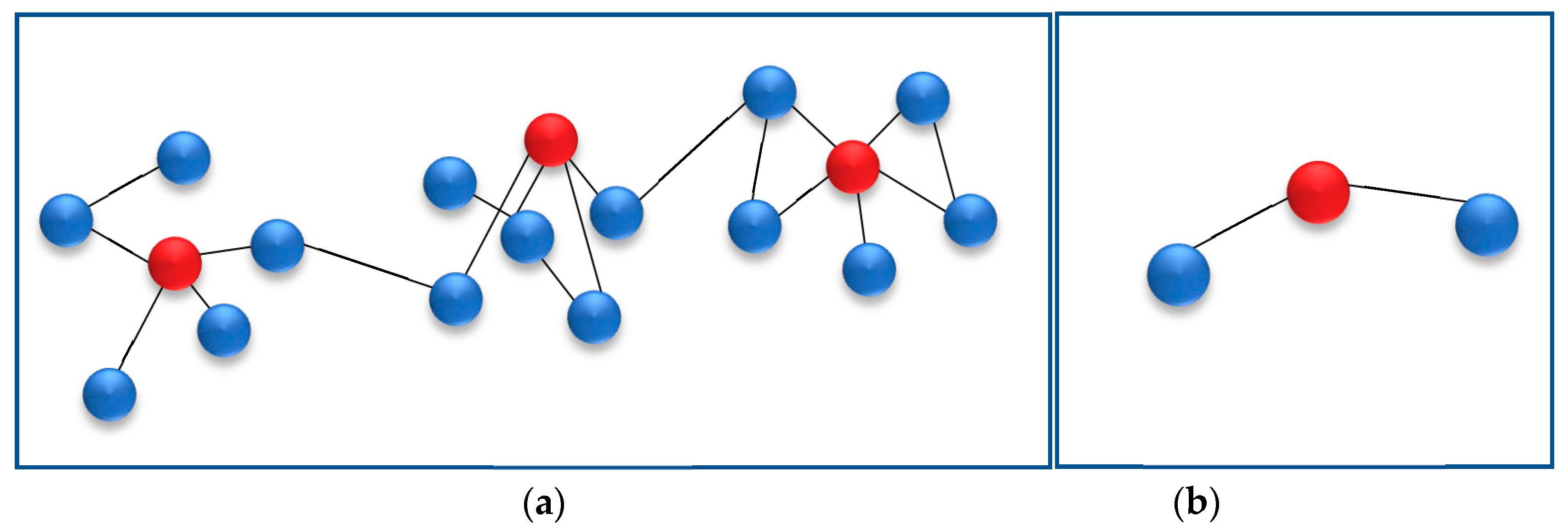
Figure 1 shows the process of constructing a hierarchical network. Figure 1a is the current level network whose red nodes represent central nodes. Central nodes condense with their neighbors (blue nodes) to form super nodes respectively, which results in the next level network as shown in Figure 1b. All super nodes in the previous level network (Figure 1a) are considered normal nodes in the next level network as shown in Figure 1b. The red node in Figure 1a will be selected as the central node, and condense with its neighbors into a super node in the next level hierarchy.
3. Algorithm Based on the Hierarchy of Networks
After transforming the original network into a number of hierarchical networks, the distance of the shortest path between any two nodes in the lower network can be estimated by considering their corresponding central nodes in the higher-level network.
Let be the approximate distance between nodes s and t in the level i network. The distance of shortest path between nodes s and t in the original network is approximated by . In general, is iteratively computed by
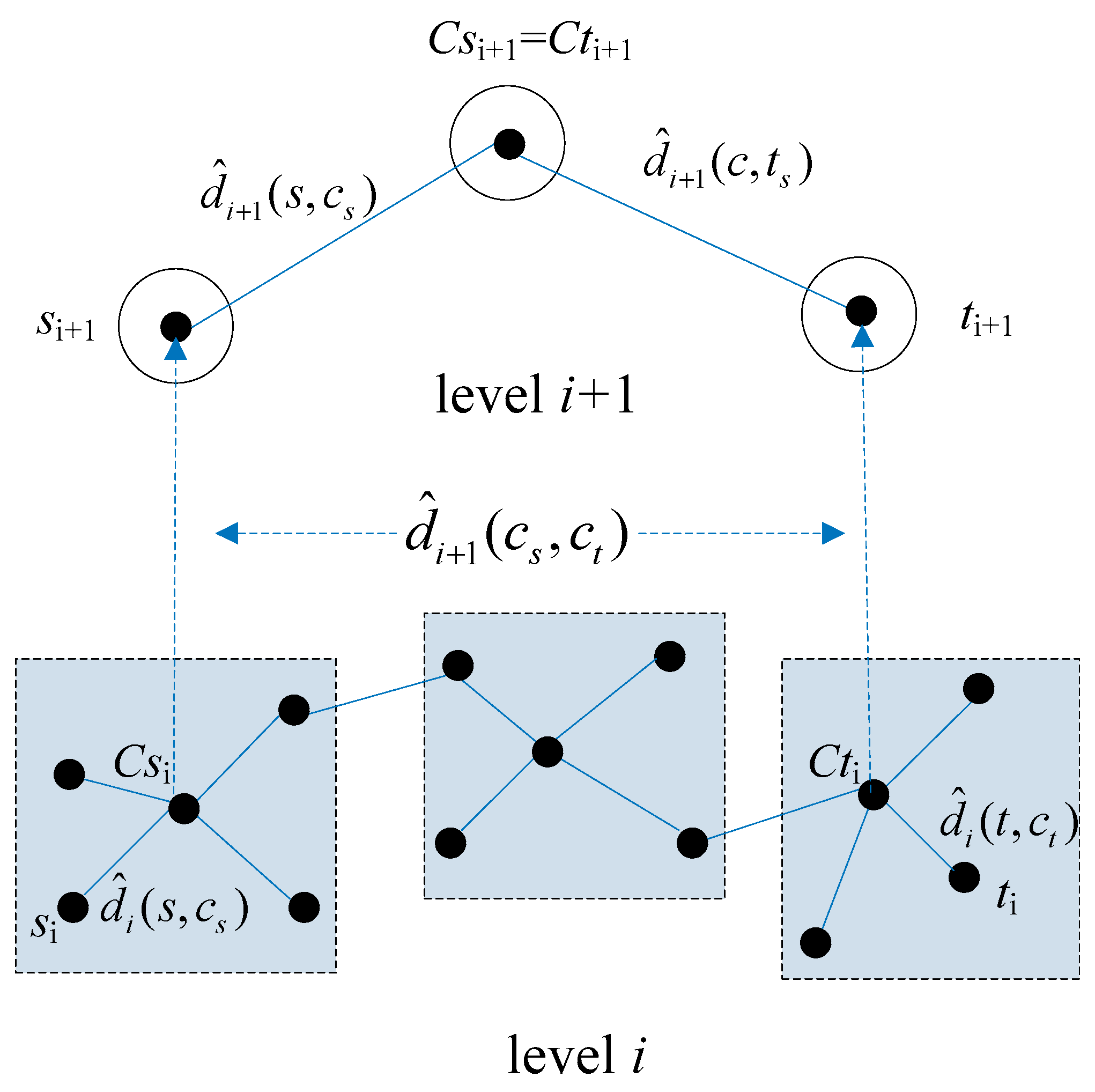
where cs and ct are the central nodes of nodes s and t respectively. Figure 2 shows an example of shortest path approximation using Equation (1). a nd are the approximate distances from nodes si and ti to their respective central nodes and in the level i network. and are the distances from nodes si+1 and ti+1 to their common central nodes in the level i + 1 network.
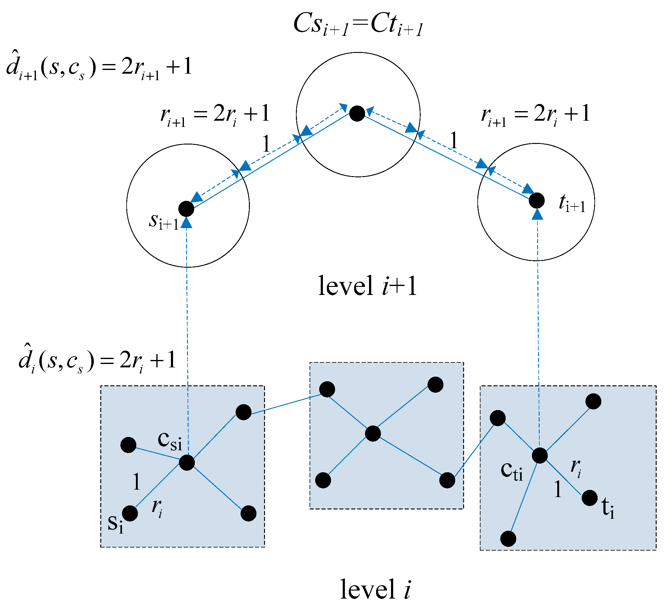
We define the longest distance from sub nodes to its corresponding central node as the radius of the super node. For example, assuming normal nodes in the level i network in Figure 2 have the same radius r, then the radiuses of their corresponding super nodes will range from r to 3r + 1 (Note: the longest path to a central node is 3r). However, computing for all radii of super nodes in the network hierarchy will consume so much memory and time. For this reason, we define an appr radius for all super nodes in the level i network by approximating the distance between two adjacent normal nodes in the level i network. As shown in Figure 3, the appr radiuses of super nodes in the level i + 1 network are the approximate distances between the centers of two adjacent normal nodes (represented as hollow circles). Normal nodes in the level i + 1 network were derived from super nodes in the level i network whose appr radiuses were same. The apprr adius of normal nodes in level i network is defined by
where k is the number of hierarchical networks with different scales including the original network. Furthermore, Equation (2) can be written as when . We approximate the distance from node s to its central node c in the level i network by
The approximate distance between adjacent nodes in level i network can also be written as . Substituting Equations (2) and (3) into Equation (1), the upper bound of can be calculated by
The distance between any two adjacent nodes in the top-level network is approximated as . in Equation (4) is the length of shortest path between nodes s and t in the top-level network computed by Dijsktra’s algorithm.
The construction of each level of the hierarchical network is described in Algorithm 1. Algorithm 1 consumes O(nilogni) time to rank the ni nodes in the level i network and O(ni + ei) time to generate the level i + 1 network, where ei is the number of edges in level i network. The space complexity of Algorithm 1 is O(n + e).
| Algorithm 1. First Hierarchy |
| Notations: is the original network, is the next level network, is the super node and its neighboring normal nodes repectively |
| 1: function SingleCluster (old) |
| 2: C←HighestDegree (old) |
| 3: for c ∈ C do |
| 4: if c S |
| 5: Sc = {c} U {c.neighbors\S} |
| 6: S←S U {Sc} |
| 7: Edges connected to the sub nodes inside Sc are redirected to Sc, also the multiple edges are merged into a single one. |
| 8: end if |
| 9: end for |
| 10: All super nodes in S are regarded as normal nodes in V′ of new. |
| 11: return new |
| 12: end function |
| 13: function HighestDegree (old) |
| 14: for each v ∈ V let d[v] ←degree (v) |
| 15: sort V by d[v] |
| 16: v(i) denotes the vertex with the i-th highest d[v] |
| 17: return sequence {v(1), v(2), ……, v(|V|)} |
| 18: end function |
4. Parallelization
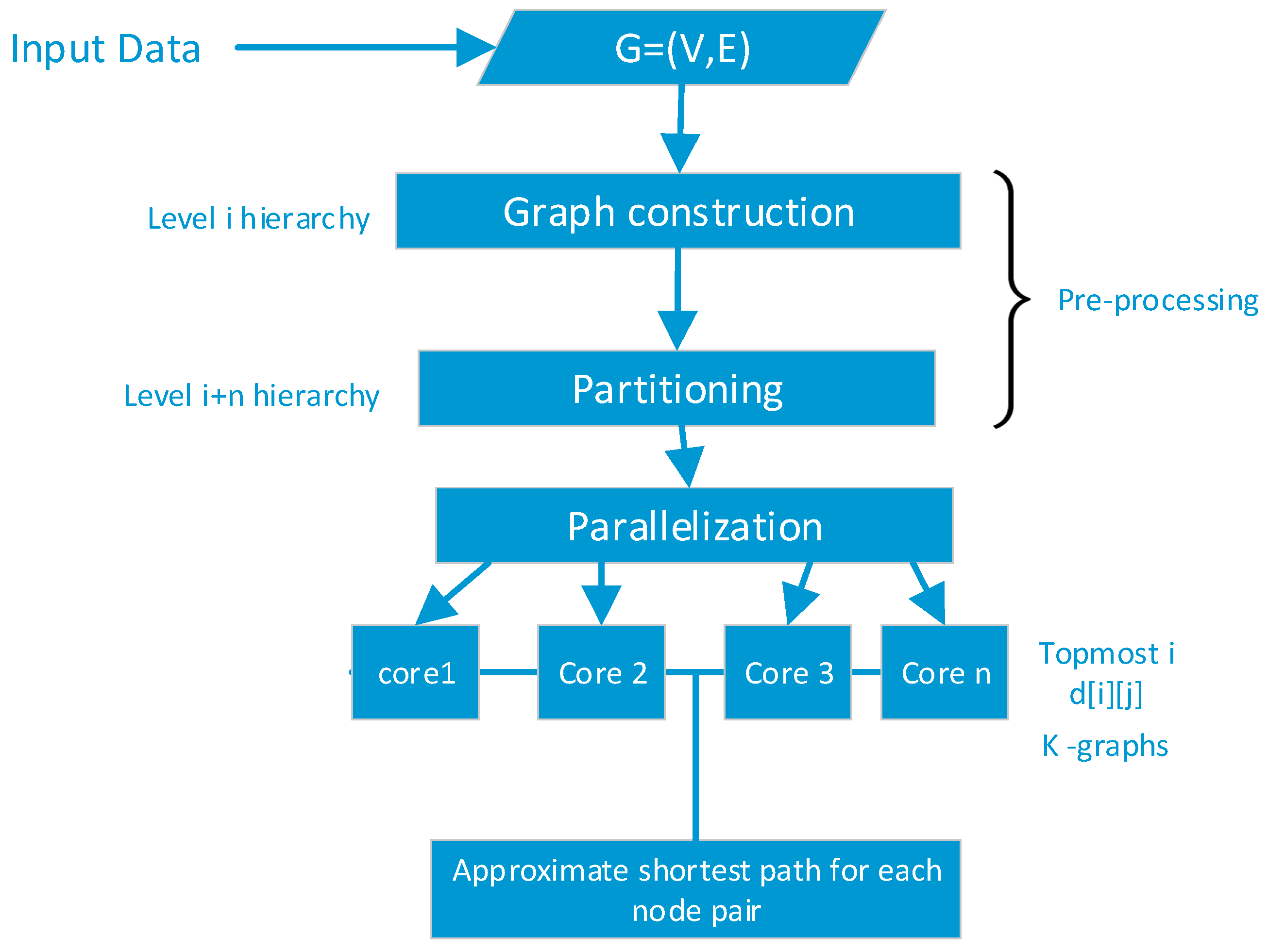
In order to reduce the overall computational runtime for computing the shortest path from to , we parallel to jobs to each processor on the computing hardware. Parallelization is simultaneously employing multiple compute resources by sharing tasks among these resources to solve a computational problem. Two common approaches to run our algorithm are via either threads or multiple processes. Threads treat each job as sub tasks of a single process and therefore would have to access the same memory location. If synchronization is not done properly, there could be conflicts for example when there is access to the same memory location at the same time. A safer approach is to submit each task to a completely separate memory location. We distribute networks evenly on to multiple cores thus passing level networks to a cpu core for computation. Dijkstra’s algorithm can only compute the shortest path from s to t after it has completed computation of shortest path where w is any vertex that satisfies It is evident that this process will increase the idleness on processors that leads to a reduction in resource utilization and efficiency [13] where efficiency was about . Figure 4 shows the architecture of the various stages of our proposed algorithm. The given network is the input data to the hierarchical graph construction process at the pre-processing stage. The graph in partitioned into k number of hierarchies and distributed across the processor cores of the computing machine.
Algorithm 2 describes the subsequent construction hierarchies. Algorithm 1 is repeatedly executed until the top-level network is achieved which is essentially equal to the partitioning value (p) nodes given a threshold (t). The time complexity for constructing hierarchical networks is given as and space complexity as . In the top level network, Dijsktra’s algorithm require time to compute the shortest paths between each pair of nodes and space to store the distances, where is the number of nodes in the top level network. Incorporating time and space complexity into Dijsktra’s algorithm requires space to store hierarchical networks and corresponding distances in the top level network.
| Algorithm 2. Hierarchy Networks |
| Preconditions: Network original = (V, E), d[i][j] records the shortest distance between node i and j in the top level network. |
| 1: Network = original |
| 2: k = Network/number_of _processors |
| 1: function HierarchyCluster |
| 2: Network current = original; |
| 3: while current.size > threshold |
| 4: If len(current) <= k |
| 5: next = SingleCluster(current);//Algorithm 1 |
| else |
| 6: current = next; |
| endif |
| 7: end while//hierarchy networks |
| 8: Employ Dijsktra’s algorithm to find shortest path between any pair of nodes on the top level network. Save the results to d[i][j]. |
| 9: return d[i][j] |
| 10: end function |
After the construction of a number of networks from Algorithm 2, Algorithm 3 distributes the networks across each processor core of the computing hardware for computation.
| Algorithm 3. Parallelization of Hierarchies |
| Input: level i networks computed by Algorithm 2. |
| Function Create Pool_Object(p) = processes |
| 1: part_generator = 4*len(p._pool) |
| 2: max_number_of_clusteres = int(len(original)/part_generator//total number of hierachies |
| 3: k = len(max_number_of _clusters) |
| 4: return k |
| 5: Distribute hierarchy networks evenly to each processor |
| 6: Parallel_mapping = p.map (btwn_pool, zip([original] *number of clusters, hierarchies)) |
| 7: Return parallel_mapping |
Finally, the approximate distances of the shortest paths in the original network can be calculated by Algorithm 4. Algorithm 4 requires at most time to compute the shortest paths for all pairs of nodes, where is the number of processor cores.
| Algorithm 4. Calculate Shortest Path |
| Preconditions: Network network = G(V, E), d[i][j] records shortest distances between nodes in the top level network calculated by Algorithm 2; k denotes the number of hierarchical networks constructed by Algorithm 2, including the original network; cs and ct are the central nodes of s and t respectively; supernode(cs) is the super node which contains nodes cs and s and its regarded as a normal node in the next level network. |
| 1: function IterativeApproximation(s,t,i) |
| 2: for i in parallel_mapping |
| 3: if i < k−1 |
| 4: if cs = ct in the level i network//hierarchy networks |
| 5: return d(s, cs)+d(t, ct)//use Equation (4) to calculate d(s, cs), d(t, ct) |
| 6: end if |
| 7: else if cs ≠ ct in the level i network |
| 8: return d(s, cs) + IterativeApproximation (supernode(cs), supernode(ct), i + 1) + d(t, ct)//Equation (4) |
| 9: end else |
| 10: end if |
| 11: else |
| 12: return d[s][t]//use the distances between nodes in the top network computed by Dijsktra in Algorithm 2 |
| 13: end else |
| 14: end function |
| 15: function CalculateshortestPath |
| 16: if s ∈ V is directly connected with t ∈ V then |
| 17: result = 1; |
| 18: end if |
| 19: else |
| 20: result = IterativeApproximation (s, t, 0)//iterative approximation for the d0(s, t) |
| 21: end else |
| 22: return result |
| 23: end function |
Based on the above analysis, the time complexity for approximating the shortest distances in an undirected and unweighted network with nodes and edges can be calculated as , and the memory complexity as .
We compared the complexity of CDZ [9] and LBFS [10] with our algorithm. CDZ algorithm selects c central areas in the network with nodes and edges and computes the distances between and its central nodes by Dijkstra’s algorithm. The time complexity of CDZ algorithm is given as . The number of central areas in CDZ algorithm is about 10% of the number of nodes. LBFS algorithm selects pairs of nodes from the network to obtain landmarks by “best coverage strategy” in a network with node and edges. The time complexity of LBFS is given as , where is the average size of the sub network related to the landmarks. Sometimes, the number of pairs of nodes in LBFS could be too large to make a best coverage and selection. The advantage of our algorithm over LBFS is that, the number of the nodes in the top network is relatively very small (m is below a certain threshold), which significantly reduces the complexity, moreover, optimum utilization of hardware and memory was realized by paralleling the computing tasks which yielded a significant improvement.
5. Completeness, Soundness and Cost Optimality
In this section, we will show that our proposed algorithm is sound, complete, and optimal. An algorithm is sound if it always returns an answer. Completeness on the other hand is the guarantee that an algorithm will always return the true results for any arbitrary inputs. Our proposed algorithm will always find the best solution to finding the shortest path even in worse case scenarios, the lower bound for the function for time complexities is used in computing the shortest path.
5.1. Sound and Completeness
Suppose we are to calculate the shortest path between two arbitrary nodes and . Our algorithm searches for their corresponding graph in the top-level hierarchy . If both nodes are contained in a super node or , the shortest path distance is approximated by the distances from their respective nodes to central nodes or and ⊃ and . For , the distances are approximated by the node s’s distance to + the distance between node and in the next higher network ) the distance from to . If , then the approximated distance between and existed within different central nodes within or across different levels of the algorithm will always search for the central nodes of and until the topmost hierarchy. If there is path between central nodes of s and t, and shortest path between and is not recorded at the topmost hierarchy, then the algorithm returns a path value of 0, which means there is no edge between and that is no path between and
5.2. Optimality
An algorithm is optimal if the time complexity for finding the solution to a problem in worst case scenario is in the lowest range of the functions that describes the time complexity in worst case scenario to the problem. Our algorithm finds the shortest path distance from the smaller graph to the largest, i.e., a top bottom approach, if the path exists in the smaller graph, the algorithm selects that path terminates. Approximation between hierarchies are performed iteratively so as optimize the task rather than searching through the entire levels of graph to select the shortest path. If a path doesn’t exist in a level hierarchy, that graph is discarded and the next level graph loaded, a smaller graph is always considered which in effect minimizes the cost. The algorithm always searches within the smallest i value(s) which contain the approximated path of the two nodes in question.
6. Experimental Results and Discussions
Our algorithm was implemented by java programming language, running on a PC with intel core i5 4300M, CPU at 2.60 GHZ dual core and a 4 GB RAM. Performance of the algorithm was evaluated on four real undirected and weighted networks; Email-Enron [14], itdk0304_rlinks [15], DBLP [16] and roadNet. Email-Enron contains about half a million email communications among users whose nodes are the email addresses of senders or receivers and edges are the communication relationships. User’s email addresses represents nodes on the dataset such that if a user i sent at least one email to another user j, then there exists an undirected edge from i to j. Tdk0304_rlinks is a CAIDA Skitter Router-Level Topology and Degree Distribution of an undirected internet router-level, which contains the relationships among nodes that access the router where the nodes are users or websites and the edges are the relationships between them. DBLP network contains information on computer science publications, in which each node corresponds to an author; two authors are connected by an edge if they have co-authored at least one publication. The roadNet is a California road traffic network composed of roads and sites network with the intersections and endpoints as nodes and the connecting roads as edges. Since most roads are unidirectional, the network graph is represented as an undirected graph. The number of nodes V, edges E, diameter of network D, average degree <k>, and the largest degree kmax of these four networks are shown in Table 1.
We use Path Ratio p to assess the accuracy of the algorithm. is defined as
where is the total number of pairs of nodes, i is the distance between pairs of nodes computed by the approximation algorithm, and is the accurate distances computed by Dijkstra’s algorithm. The value of is always greater than 1 since approximate distances are always longer than their corresponding accurate distances. Table 2 shows experimental results on preprocess time, average query time, and path ratio from our algorithm compared with that of CDZ. The threshold value is set at 100. Tinit is the total time for preprocessing. Tq is the average runtime for 10,000 random queries. From table 2, it can be construed that our algorithm performed relatively better on four different networks. It ran 10 times faster than CDZ especially on DBLP and roadNet networks. Moreover, the approximation for the shortest path is more accurate on Email-Enron and itdk0304_rlinks, compared with CDZ on DBLP and roadNet.
Table 3 shows results from LCA, LBFS, and our algorithm. It can be seen from Table 3 that our algorithm outperforms LBFS in terms of efficiency and accuracy. In DBLP and roadNet, our algorithm ran twice as fast as LBFS. Compared with LCA, our algorithm approximates more accurately but with a slightly higher runtime. Moreover, parallelization improved the runtime by about 15% compared with the latter which computed shortest paths sequentially.
From our experiments, we deduced that threshold t affects the efficiency and accuracy of our algorithm. Table 4 shows the influence of threshold t. From Table 4, it can be seen that runtime increases and path ratio decreases when threshold is increased. When there are more nodes at the top level network, approximation is more accurate but requires more time for Dijkstra’s algorithm. When t increases from 40 to 100, Tq also increases a little, but p improves significantly. When the threshold value increases from 100 to 180, Tq increases sharply, but p remains nearly constant. We therefore set the threshold value at 100 in order to obtain a good trade-off.
7. Conclusions
Based on hierarchical networks, we propose a parallel approximate shortest path algorithm which is efficient and maintains high approximation accuracy on large scale networks. The algorithm condenses central nodes and their neighbors into super nodes to iteratively construct higher level networks until the scale of the top level meets a set threshold value. The algorithm approximates the distances of the shortest paths in the original network by means of super nodes in the higher-level network. The performance of our algorithm was tested on four real networks. Results from our tests show that our algorithm has a runtime per query within a few milliseconds and at the same time delivers high accuracy on large scale networks. Compared with other algorithms, our algorithm runs twice as fast as LBFS and over 10 times faster than CDZ.
The proposed algorithm mainly focuses on undirected and unweighted networks. In the future, we seek to focus on directed and weighted networks by exploring the approximate distance between a node and its central node based on hierarchical networks. We will also consider an adaptive algorithm for dynamic networks.
Author Contributions
Conceptualization, D.N.A.M.; Data curation, L.W.Y.; Investigation, D.N.A.M.; Software, D.N.A.M. and L.W.Y.; Supervision, H.G.; Writing—original draft, D.N.A.M. All authors have read and agreed to the published version of the manuscript.
Funding
This research received no external funding.
Acknowledgments
This work was partially supported by the National Natural Science Foundation of China under Grant No. 61433014, by the National High Technology Research and Development Program under Grant No. 2015AA7115089.
Conflicts of Interest
The authors declare no conflict of interest.
References
- Stolfo, S.J.; Hershkop, S.; Wang, K.; Nimeskern, O.; Hu, C.W. Behavior profiling of email. In Proceedings of the 1st NSF/NIJ Conference on Intelligence and Security Informatics, Tucson, AZ, USA, 2–3 June 2003; pp. 74–90. [Google Scholar]
- Schwarzkopf, Y.; Rákos, A.; Mukamel, D. Epidemic spreading in evolving networks. Phys. Rev. E 2020, 82, 036112. [Google Scholar] [CrossRef] [PubMed] [Green Version]
- Yang, Y.B.; Li, N.; Zhang, Y. Networked data mining based on social network visualizations. J. Software 2008, 19, 1980–1994. [Google Scholar] [CrossRef] [Green Version]
- Qiao, S.J.; Tang, C.J.; Peng, J.; Liu, W.; Wen, F.L.; Qiu, J.T. Mining key members of crime networks based on personality trait simulation email analysis system. Chin. J. Comput. 2008, 31, 1795–1803. [Google Scholar] [CrossRef]
- Freeman, L.C. Centrality in social networks conceptual clarification. Soc. Network 1978, 1, 215–239. [Google Scholar]
- Chow, E. A graph search heuristic for shortest distance paths. In Proceedings of the Twentieth National Conference on Artificial Intelligence, Pittsburgh, PA, USA, 9–13 July 2005. [Google Scholar]
- Rattigan, M.; Maier, M.J.; Jensen, D. Using structure indices for efficient approximation of network properties. In Proceedings of the 12th ACM SIGKDD International Conference on Knowledge Discovery and Data Mining, Philadelphia, PA, USA, 22–23 August 2006; Association for Computing Machinery: New York, NY, USA, 2006; pp. 357–366. [Google Scholar]
- Tang, J.T.; Wang, T.; Wang, J. Shortest Path Approximate Algorithm for Complex Network Analysis. J. Softw. 2011, 22, 2279–2290. [Google Scholar] [CrossRef]
- Tretyakov, K.; Armas-Cervantes, A.; García-Bañuelos, L.; Vilo, J.; Dumas, M. Fast fully dynamic landmark-based estimation of shortest path distances in very large graphs. In Proceedings of the 20th ACM International Conference on Information and Knowledge Management (CIKM ’11), Glasgow, UK, 24–28 October 2011. [Google Scholar] [CrossRef] [Green Version]
- Maleki, S.; Nguyen, D.; Lenharth, A.; Garzarán, M.; Padua, D.; Pingali, K. DSMR: A Parallel Algorithm for Single-Source Shortest Path Problem. In Proceedings of the 2016 International Conference on Supercomputing (ICS ’16), Istanbul, Turkey, 1–3 June 2016; pp. 1–14. [Google Scholar]
- Hart, P.; Nilsson, N.; Raphael, B. A Formal Basis for the Heuristic Determination of Minimum Cost Paths. IEEE Trans. Syst. Sci. Cybern. 1968, 4, 100–107. [Google Scholar] [CrossRef]
- Geisberger, R.; Sanders, P.; Schultes, D.; Delling, D. Contraction Hierarchies: Faster and Simpler Hierarchical Routing in Road Networks. In International Workshop on Experimental and Efficient Algorithms; McGeoch, C.C., Ed.; Springer: Berlin, Germany, 2008. [Google Scholar]
- Lanthier, M.; Nussbaum, D.; Sack, J.-R. Parallel implementation of geometric shortest path algorithms. Parallel Comput. 2003, 29, 1445–1479. [Google Scholar] [CrossRef] [Green Version]
- Klimmt, B.; Yang, Y. Introducing the Enron corpus. In Proceedings of the First Conference on Email and Anti-Spam, Mountain View, CA, USA, 30–31 July 2004. [Google Scholar]
- Broido, A. Internet topology: Connectivity of IP graphs. In Scalability and Traffic Control in IP Networks; Fahmy, S., Park, K., Eds.; SPIE: San Francisco, CA, USA, 2001; pp. 172–187. [Google Scholar]
- Ley, M.; Reuther, P. Maintaining an Online Bibliographical Database: The Problem of Data Quality. In Proceedings of the Extraction et Gestion des Connaissances 2006 (EGC 2006), Lille, France, 17–20 January 2006; pp. 5–10. [Google Scholar]
Figure 1.
Construction of hierarchical networks. (a) graph at level i, (b) level i + 1 network.

Figure 2.
Illustration of iterative approximation.

Figure 3.
Illustration of approximate distance ri.

Figure 4.
Architecture of the algorithm for computing shortest path.


Table 1.
Basic information of four networks.
| Email-Enron | itdk0304_rlinks | DBLP | roadNet | |
|---|---|---|---|---|
| V | 36,692 | 190,914 | 511,163 | 1,405,790 |
| E | 367,662 | 1,215,220 | 3,742,140 | 23,442,590 |
| D | 12 | 24 | 25 | 30 |
| <k> | 10.020 | 6.365 | 7.320 | 9.433 |
| kmax | 1383 | 1071 | 976 | 1244 |
Table 2.
Runtime and accuracy of CDZ and our algorithm on four networks.
| Graph | Our Algorithm | CDZ | ||||
|---|---|---|---|---|---|---|
| Network | Tinit (ms) | Tq (ms) | p | Tinit (ms) | Tq (ms) | p |
| Email-Enron | 10,919.21 | 1.1720 | 1.022 | 112,448 | 11.38 | 1.026 |
| itdk0304_rlinks | 46,723.65 | 4.7413 | 1.020 | 1,092,348 | 109.34 | 1.023 |
| DBLP | 87,657.1 | 8.8196 | 1.020 | 8,623,459 | 862.44 | 1.020 |
| roadNet | 167,074.3 | 16.7218 | 1.019 | 18,824,559 | 1882.55 | 1.019 |
Table 3.
Results from LCA, LBFS and our algorithm.
| Graph | Our Algorithm | LCA | LBFS | |||
|---|---|---|---|---|---|---|
| Network | Tq (ms) | p | Tq (ms) | p | Tq (ms) | p |
| Email-Enron | 1.1720 | 1.022 | 0.84 | 1.095 | 1.29 | 1.030 |
| itdk0304_rlinks | 4.7413 | 1.020 | 3.57 | 1.083 | 5.60 | 1.028 |
| DBLP | 8.8196 | 1.020 | 6.35 | 1.072 | 15.99 | 1.025 |
| roadNet | 16.7218 | 1.019 | 10.70 | 1.067 | 37.89 | 1.022 |
Table 4.
Comparison of different thresholds.
| Network | Threshold | |||||
|---|---|---|---|---|---|---|
| Parameter | 40 | 60 | 100 | 140 | 180 | |
| Email-Enron | Tq (ms) | 0.46 | 0.661 | 1.170 | 2.021 | 3.875 |
| p | 1.03 | 1.024 | 1.02 | 1.02 | 1.02 | |
| itdk0304_rlinks | Tq (ms) | 2.31 | 3.65 | 4.72 | 8.04 | 15.56 |
| p | 1.03 | 1.026 | 1.02 | 1.019 | 1.018 | |
| DBLP | Tq (ms) | 5.49 | 7.521 | 8.78 | 17.214 | 36.820 |
| p | 1.03 | 1.022 | 1.02 | 1.018 | 1.018 | |
| roadNet | Tq (ms) | 10.89 | 13.10 | 16.79 | 33.41 | 61.58 |
| p | 1.026 | 1.02 | 1.02 | 1.018 | 1.018 | |
© 2020 by the authors. Licensee MDPI, Basel, Switzerland. This article is an open access article distributed under the terms and conditions of the Creative Commons Attribution (CC BY) license (http://creativecommons.org/licenses/by/4.0/).
Share and Cite
MDPI and ACS Style
Mensah, D.N.A.; Gao, H.; Yang, L.W. Approximation Algorithm for Shortest Path in Large Social Networks. Algorithms 2020, 13, 36. https://0-doi-org.brum.beds.ac.uk/10.3390/a13020036
AMA Style
Mensah DNA, Gao H, Yang LW. Approximation Algorithm for Shortest Path in Large Social Networks. Algorithms. 2020; 13(2):36. https://0-doi-org.brum.beds.ac.uk/10.3390/a13020036
Chicago/Turabian StyleMensah, Dennis Nii Ayeh, Hui Gao, and Liang Wei Yang. 2020. "Approximation Algorithm for Shortest Path in Large Social Networks" Algorithms 13, no. 2: 36. https://0-doi-org.brum.beds.ac.uk/10.3390/a13020036
Note that from the first issue of 2016, this journal uses article numbers instead of page numbers. See further details here.