1. Introduction
Control systems encounter unpredictable disturbances in real-world control applications. In order to maintain optimal control performance, real control systems should be designed to be robust enough against environmental disturbances, which are mainly unpredictable in character. From a practical point of view, performance degradations of classical control systems are largely caused by their dependence on predetermined system models. In the controller design phase, classical PID controllers are tuned to produce optimal control of a predetermined nominal plant model, which is indeed an idealized representation of a real-world system. The mathematical models of real systems can maintain their validity for predefined operating conditions and ranges, and only observable dynamics of the systems in these range and conditions can be represented by system models. Hence, they omit some inaccessible system dynamics and unknown disturbances, which are not rigorously investigated in the modeling stage. To enhance the representative capability of mathematical modeling, it is well-known that non-linear modeling [
1], fractional-order modeling [
2], and stochastic modeling [
3] methods are often used. However, nowadays, optimal PID tuning methods still rely on integer order dynamics and linear system design approaches for the sake of simplicity and practical effectiveness. Therefore, the coverage potential of these modeling types to represent real-world conditions is quite limited, while mathematical models can represent the behavior of real systems in some presumed idealized conditions.
In general, optimal controller design in classical control has been addressed using integer order plant models and linear dynamics. Consequently, the designed controller law becomes mathematically optimal only for those ideal and linearized models operating in numerical simulation environments. However, when they are implemented in real-world conditions, practitioners commonly encounter the fact that the calculated controller coefficients are not practically optimal for real processes and fine-tuning efforts are needed for these controllers to achieve acceptable control performance. Firstly, non-ideal realization of controller function inherently deteriorates control optimality. Secondly, a number of factors such as unmodelled dynamics, noise, environmental disturbance, ageing of system components, and parametric perturbations may have a significant influence on control performance. Therefore, it is obvious that model-based optimal controller design methods should adhere to robust control performance requirements in the controller design stage, including considerations of disturbance rejection performance and insensitivity to model parameter variation. The current study focuses on enhancement of the disturbance rejection performance of classical control loops. The disturbance model is assumed to be additive input disturbance that has unknown characteristics. The disturbance rejection capacity of a classical negative feedback PID control loop is inherently bound [
4]. A feasible solution to increase disturbance rejection performance beyond the inherent bounds of a PID control loop is by using a multi-loop control structure [
5]. The findings of the current study suggest that a multi-loop model reference (ML-MR) adaptive control structure could be an effective solution to improve the disturbance rejection performance of classical PID control loops.
Due to a performance tradeoff between disturbance rejection control and set-point control performances [
4], increasing the disturbance rejection control performance can severely deteriorate the set-point performance of classical PID control loops. A primary motivation of this study is the improvement of disturbance rejection control performance without effecting the set-point performance of existing closed loop PID control systems.
ML-MR control structures are commonly composed of two hieratical loops. These are the reference model loop, which describes the desired response of a system, and the control loop, which deals with the stability of control systems. The control loop is the primary loop that maintains the stability of the system. The secondary loop is the reference model loop, also called the adaptation loop, which handles the preservation of the desirable control performance of the system, which is described by the reference model response. When a disturbance acts on the control loop, the adaptation loop contributes to the control efforts for the reduction of the negative effects of disturbances on system outputs, thus restoring control performance by means of reference responses that are generated by the reference model.
In literature, numerous ML-MR control structures have been proposed and their improvements in terms of control performance have been demonstrated. In former works, direct model reference adaptive control (MRAC) structures have been addressed [
5,
6,
7,
8,
9,
10]. Direct MRAC structures perform online self-tuning of controller parameters according to a predefined reference model [
5,
6,
7,
8]. Updating controller parameters in control action, known as online controller tuning, may lead to short-term instability and control performance degradations. Therefore, the stability and robust control performance of MRAC structures in real conditions remain questionable and direct MRAC control methodologies have not been accepted or adopted by practitioners [
8]. The industrial applications of the MRAC method have remained limited in comparison to the widespread adoption of classical PID control loops. PID control loops have been used as industrial standard control systems because of their well-established design scheme. The simple structure and reliability of PID control law, which facilitates realization in real systems, are prominent in industrial control applications. Barkana has addressed performance and stability issues of direct MRAC methods and presented a stable direct MRAC methodology according to passivity conditions [
8]. However, to avoid online controller parameter updates in control action, one branch of ML-MR control research studies aims to combine a classical PID control system with reference model control in a hierarchical multi-loop manner in order to benefit from the stability and set-point performance of the classical control loop and the robust control performance improvements of the model reference control (MRC) system.
The topic of multi-loop control involves a wide variety of control systems that employ multi-loop control structures, including cascaded control loops [
11,
12], multi-input multi-output control systems [
13], use of additional control loops for performance improvements [
14,
15], direct model reference control based on output matching [
16,
17], direct model reference adaptive control with online controller tuning [
5,
6,
7,
8,
9,
10], model reference adaptive control based on Massachusetts Institute of Technology (MIT) rule [
18,
19,
20,
21,
22,
23], backstepping-based adaptive PID control [
24], and hierarchical ML-MR adaptive control [
25,
26,
27,
28]. The current study investigates several configurations of hierarchical ML-MR adaptive control structures.
Hierarchical ML-MR adaptive PID control has been investigated, and certain benefits of this structure related to fault tolerance [
25] and disturbance rejection [
26] have been discussed. This structure can be easily applied to the existing closed loop PID control systems, thus transforming the PID control systems into model reference adaptive PID control systems. This presents a significant potential to improve the robust control performance of industrial PID control systems without largely modifying the existing PID loops. Although a growing research trend has been initiated for the use of ML-MR adaptive PID structures to improve the control performance of the closed loop PID control family [
25,
26,
27], this control structure is still in the early stages of development. There is a need for further research efforts to establish design methodologies and reveal some practical benefits and drawbacks. Therefore, this study aims to investigate the benefits and drawbacks of ML-MR PID-MIT control [
25,
28] and addresses design and performance improvement problems in ML-MR structures. To this end, this paper revisits recent multi-loop model reference adaptive PID control techniques, and analytical tuning and performance issues are considered. In analytical optimal tuning of PID controllers, we adopt the integral time absolute error (ITAE) design rule that was proposed by Tavakoli et al. for control of the first order plus dead time dynamic systems. This design rule is based on dimensional analysis, which has been widely utilized to solve complex high-dimensional problems by reducing the number of variables to an essential set [
29]. The main reason to use the Tavakoli–Tavakoli ITAE design rule for optimal tuning of PID control loops is that the method limits overshoot with faster establishment of set-point control in time delay systems [
29].
The organization of this paper is given as follows.
Section 2 details the mathematical background of the multi-loop model reference PID-MIT (ML-MR PID-MIT) control, and presents analytical equations for theoretical background and analytical tuning. After discussing some inherent drawbacks of ML-MR PID-MIT structures (e.g., nonlinearity and amplitude dependence of disturbance rejection performance), several ML-MR control structures are investigated to resolve these drawbacks in the following sections. In these sections, two types of hierarchical ML-MR control structures are considered.
(i) Reference modeling of closed loop control loops: These types of MRC structures use a reference model to describe the desired response of closed loop control systems.
Section 3 presents a multi-loop model reference PID-MIT control with controller gain modification (ML-MR PID-MIT-CGM) that allows dynamic disturbance rejection via adaptively adjusting Reference to Disturbance Ratio (RDR) performance. To deal with the drawbacks of nonlinearity from the MIT rule, a multi-loop model reference PID integral (ML-MR PID-I) control, which performs a linear adaptation rule, is introduced in this section.
Section 4 introduces a multi-loop model reference PID-IM control structure (ML-MR PID-IM) that is proposed as an internal model linear adaptation rule to implement an internal model control (IMC) approach.
(ii) Reference modeling of plants: These types of MRC structures use a reference model to describe desired responses of a process or a plant function.
Section 5 presents the multi-loop model reference MIT-PID control, which employs the model reference control rule only for plant function adaptation (ML-MR MIT-PID-PFA) in contrast to ML-MR MIT-PID in
Section 2. The main advantages of this type of structure come from the fact that all adaptation efforts aim for approximation of plant or process models compared to the reference model. This property is advantageous for time delay systems.
Section 6 presents a multi-loop model reference PID-PID control with plant function adaptation (ML-MR PID-PID-PFA). This structure employs a linear adaptation rule for plant function and it can improve control performance for time delay systems.
Illustrative design examples cover control the problems of an automatic voltage regulator model, the liquid level of reboilers, large time delay experimental process models, and Twin-Rotor Multi-input multi-output System (TRMS) experimental setup.
2. Multi-Loop Model Reference PID-MIT (ML-MR PID-MIT) Control: Analytical Tuning and Nonlinearity
The ML-MR PID-MIT control structure has been proposed to enhance the robust control performance of existing closed loop control systems. Its application has been discussed in several works [
25,
26,
27,
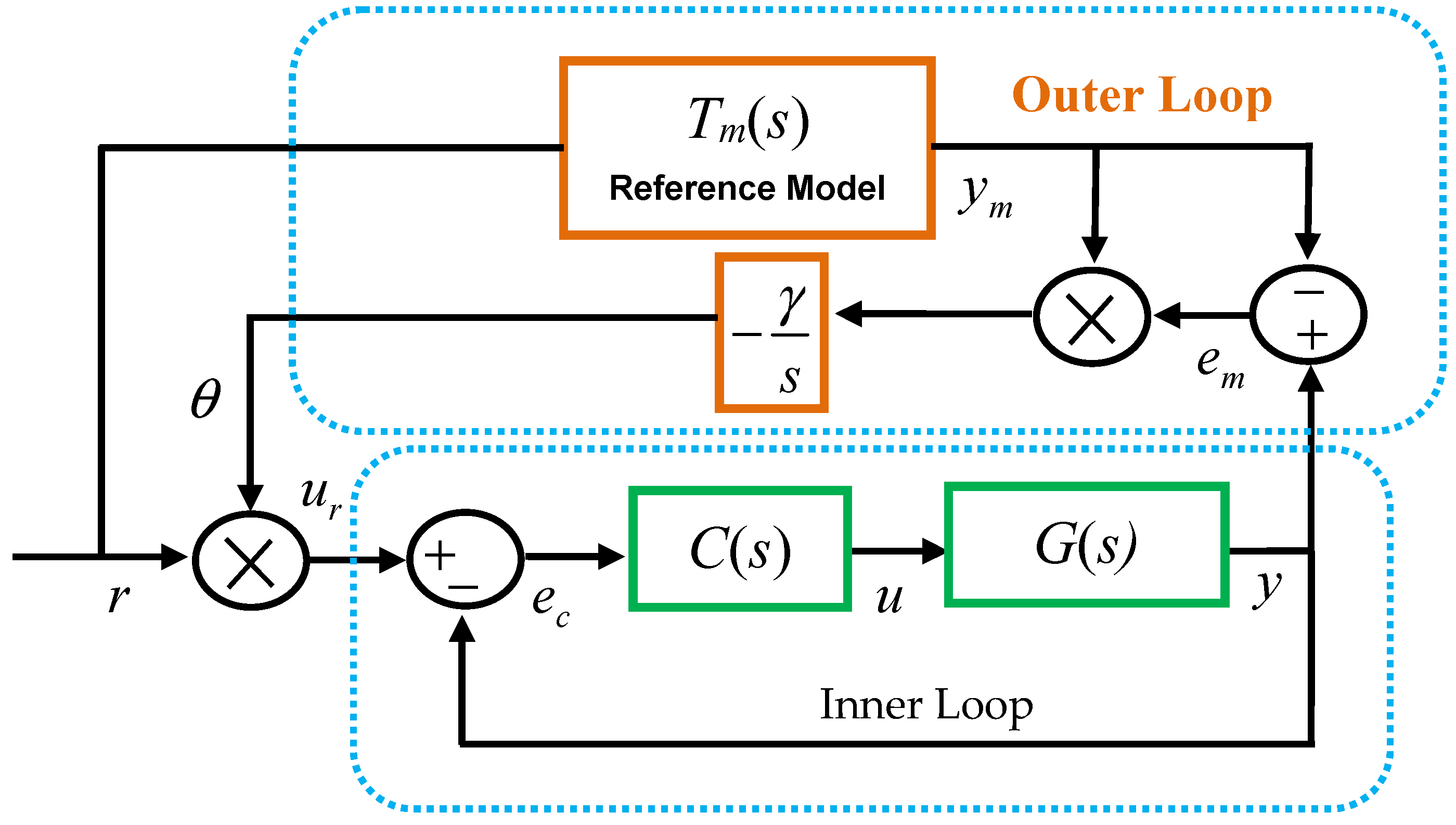
28]. This structure is essentially composed of two hierarchical control loops: the inner loop is a classical PID control loop that is a stable and well-tuned control loop, while the outer loop is a adaptation loop that performs the MIT rule. The outer loop is appended to the inner loop to enhance the robust control performance of the inner loop according to regulation of a reference model.
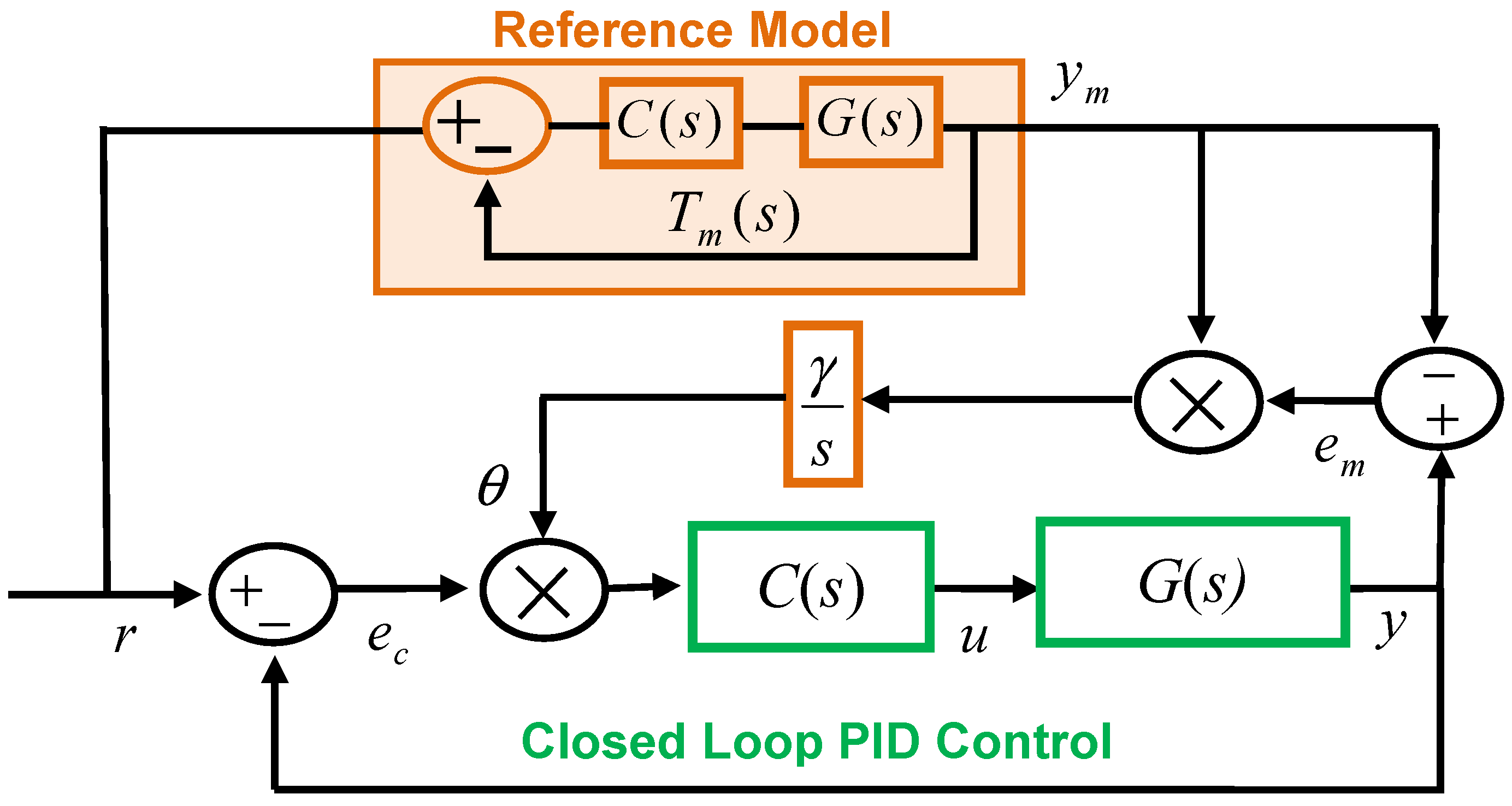
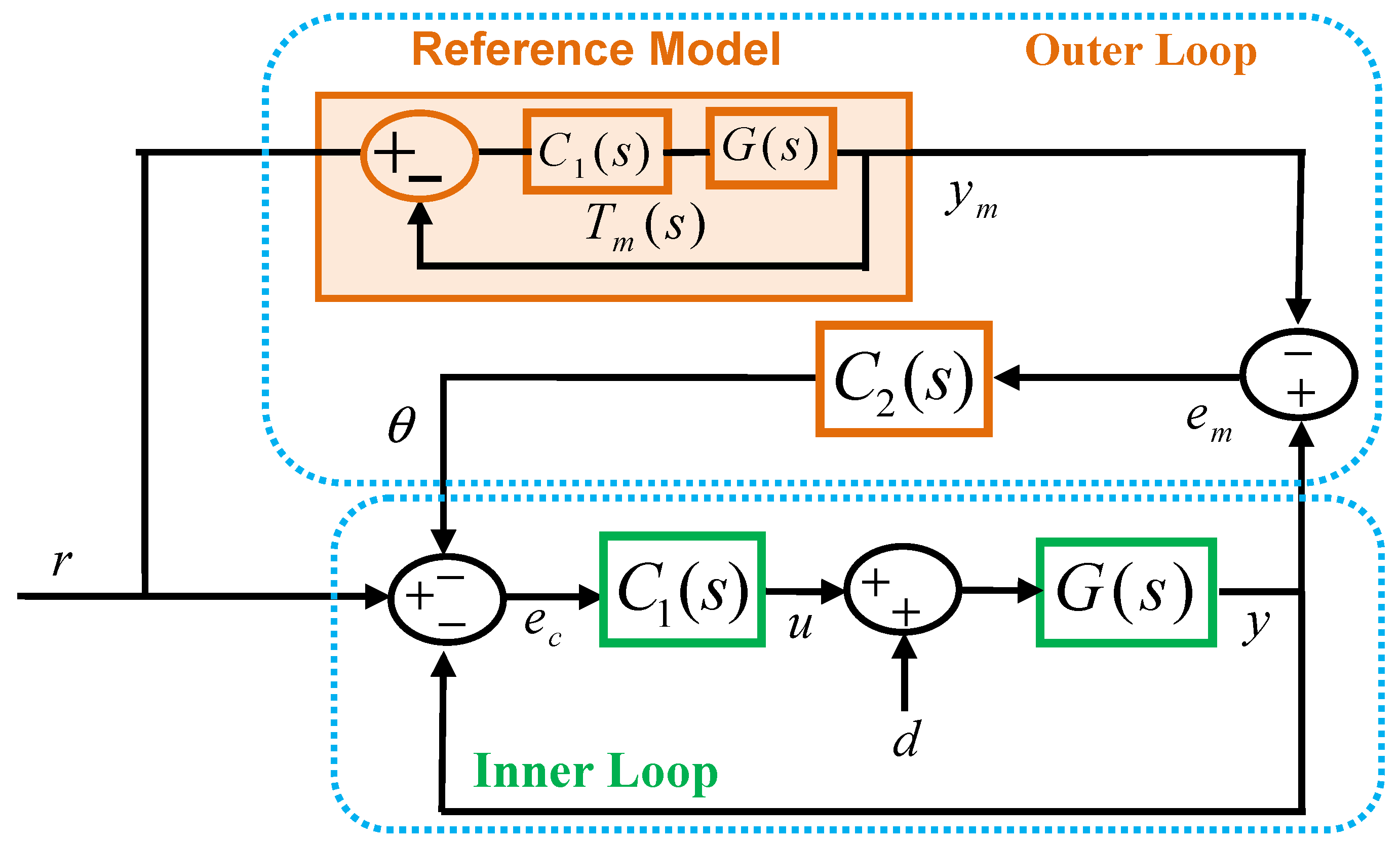
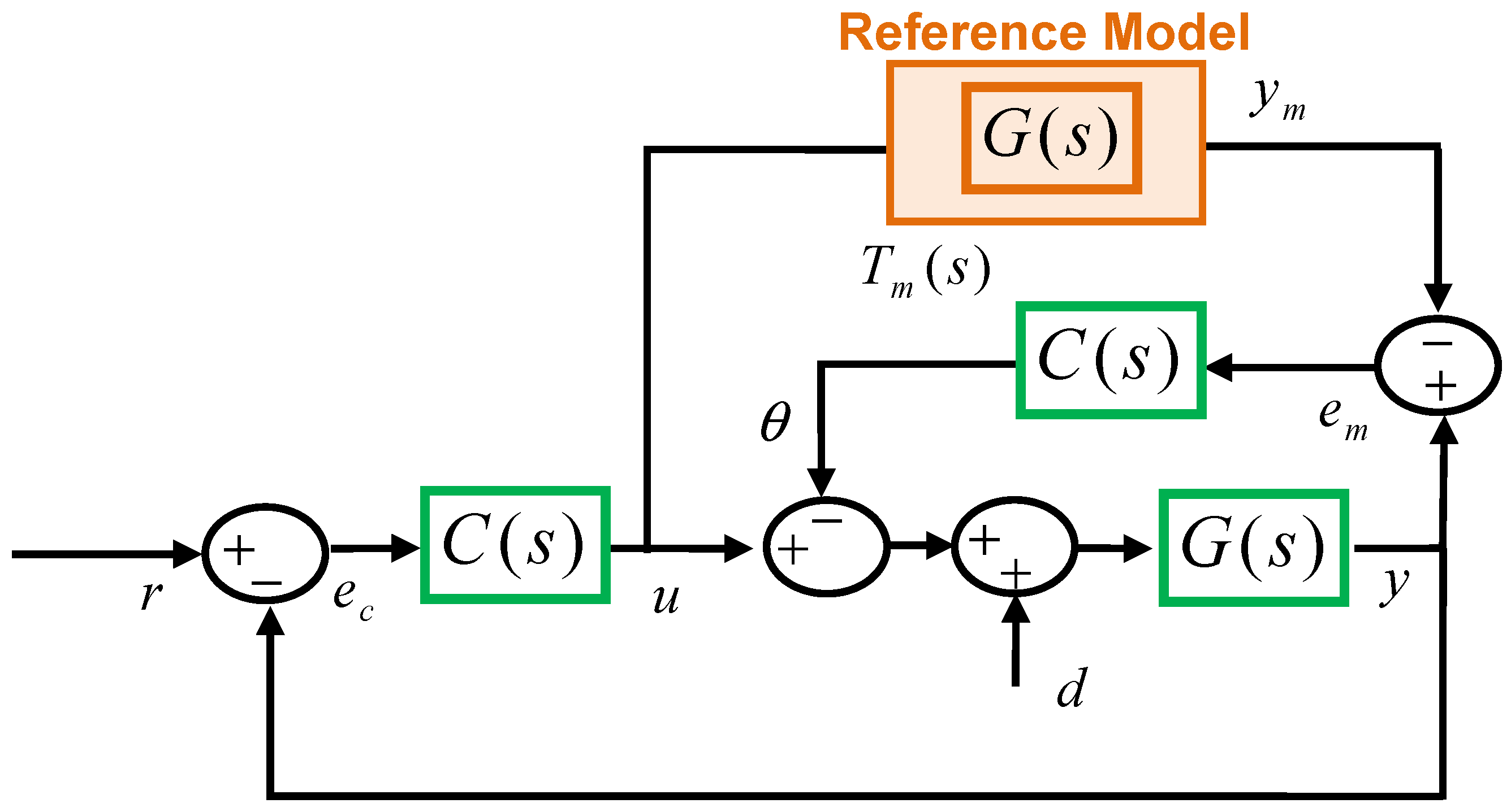
Figure 1 shows a block diagram of the ML-MR PID-MIT control structure. It has two error signals per loop:
- (i)
Control error: When the controller of the inner loop is tuned properly, the value of the control error, which is written as , moves to zero, and thus ensures the control system output settles to the reference input (the signal is the modified reference input controlled by the MIT rule and is the system output).
- (ii)
Model error: Discrepancy between the reference model output and controlled system output is defined as the model error, which is written as (the signal is the output of reference model). The objective of the outer loop is to shape the reference input signal () such that the model error converges to zero. The convergence of the model error to zero implies that the inner loop resembles the response of the reference model . The reference model describes the desired response of the control system that forms the inner loop.
Let us consider a PID control system as the inner control loop. The PID controllers are three-coefficient standard industrial controllers and optimal tuning of the PID coefficients (
,
,
) enhances step performance by reducing overshoots and settling time. The transfer function of PID controllers is widely expressed in the parallel form as:
For a given plant (process) function
, the transfer function of the inner loop can be written by:
Previous studies on the ML-MR PID-MIT control structure aim to maintain the initial well-tuned control performance of an existing closed loop control system. For this reason, the reference model is taken as the transfer function of the inner loop; that is,
. Accordingly, any performance deterioration in the inner loop leads to an increase in model errors. The recovery of temporal performance deterioration is carried out by shaping the reference input of the inner loop via
. The adaptation gain
is determined according to the well-known MIT rule [
21], which implements continuous gradient descent optimization of the cost function:
The feed-forward MIT rule is expressed in the continuous domain as [
18,
19,
20,
21]:
where the parameter
is the learning rate, which is an important parameter for the convergence speed and stability of the gradient descent optimization. Taking Laplace transform of Equation (4), one obtains:
To find the sensitivity derivative
, the model error is written in the form of
. Then, the sensitivity derivative of the system is obtained:
Here, one can substitute the reference input with
in Equation (6) and rearrange the sensitivity derivative as:
By using it in Equation (5), the MIT rule for the update of the adaptation coefficient
to minimize cost function
is obtained as [
25,
26,
28]:
When one configures
, the adaptation gain
is simplified to:
which is implemented in the outer loop in
Figure 1 [
25,
26,
28].
Application of ML-MR PID-MIT control for the existing control loop was defined as follows [
25,
26,
28]:
Step 1: Identify the transfer function model of the existing closed loop PID control system by means of closed loop model identification methods and use this transfer function as a reference model.
Step 2: Enclose the existing closed loop control system via the outer loop. The outer loop employs Equation (9) and the reference model control.
To create a design from scratch for a first order system model in the form of , an analytical tuning scheme for the ML-MR PID-MIT control structure can be proposed as follows:
Step 1: Design a closed loop PID control system according to the Tavakoli–Tavakoli PID tuning rule that can be rearranged for a standard PID controller function in parallel form as follows [
29]:
This optimal tuning rule implements ITAE and its control performance have been shown previously [
29]. The optimal PID controller function of the inner loop can be written for the Tavakoli-Tavakoli optimal PID tuning rule as:
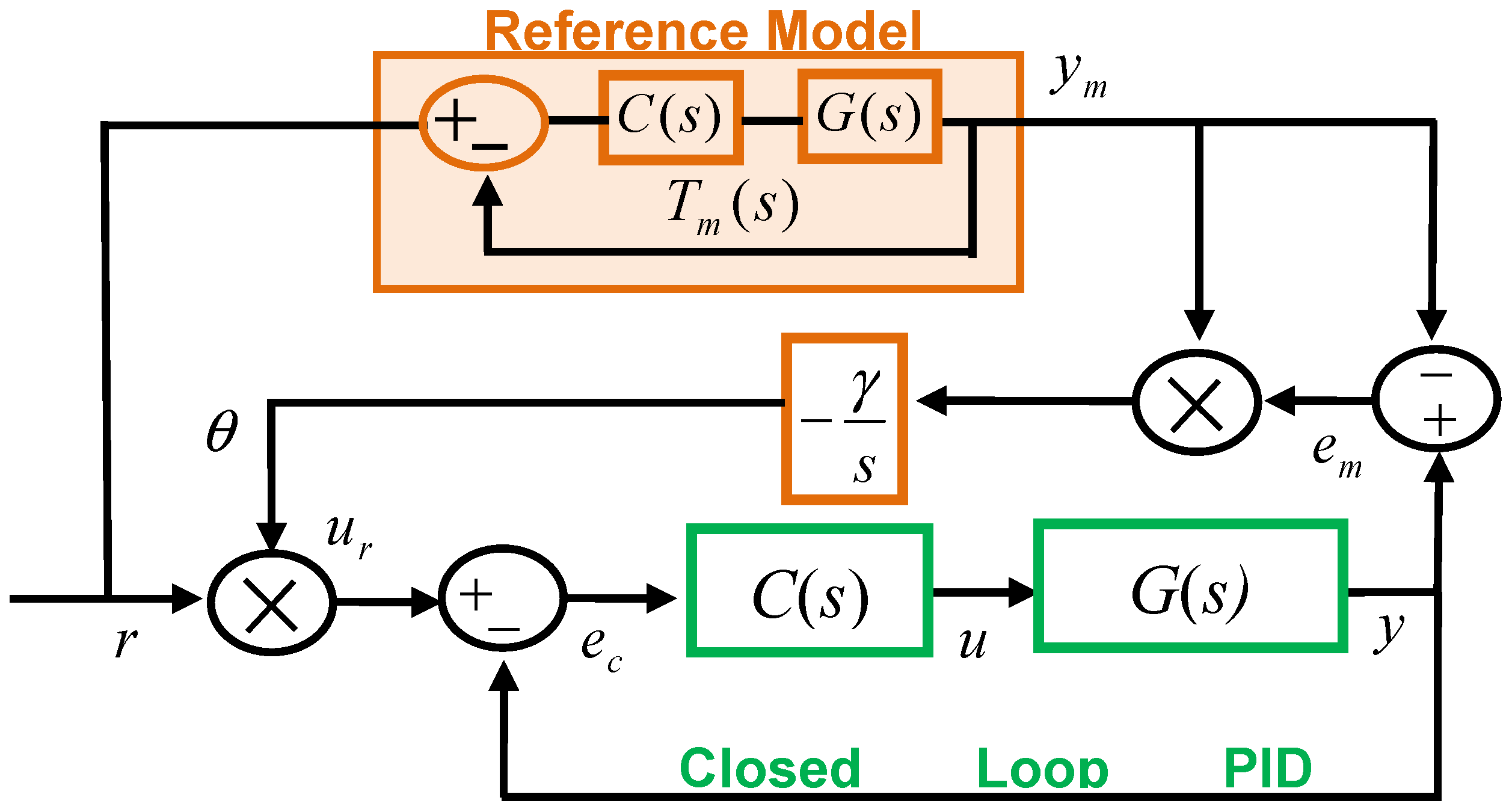
Step 2: The reference model is a theoretical model that represents the optimally tuned closed loop control system. Therefore, the transfer function of reference model can be expressed as:
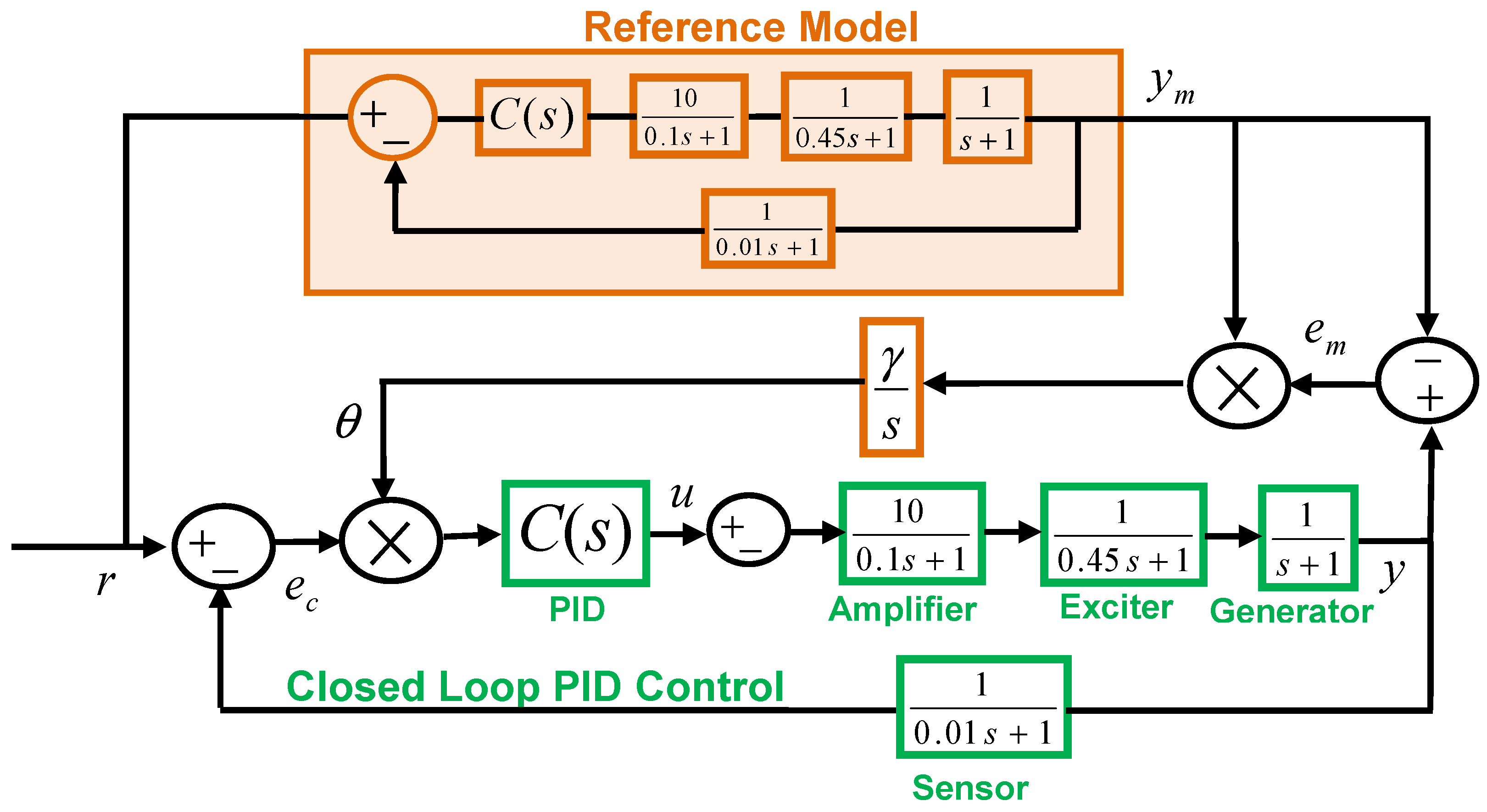
In MATLAB and Simulink control system simulations, we implemented this reference model as a numerical model of the PID control loop, as illustrated in the diagram in
Figure 2.
Step 3: Implement the ML-MR PID-MIT control structure as shown in
Figure 2. The learning rate
can be selected to comply with integral dynamics of the PID control loop.
It is important to note two characteristic features of this structure. Firstly, the performance of the ML-MR PID-MIT control structure is sensitive to the time delay component of the system. As the time delay of the system increases, the adaptation performance of the MIT rule decreases because large delay in the system response easily misleads gradient descent optimization of the MIT rule.
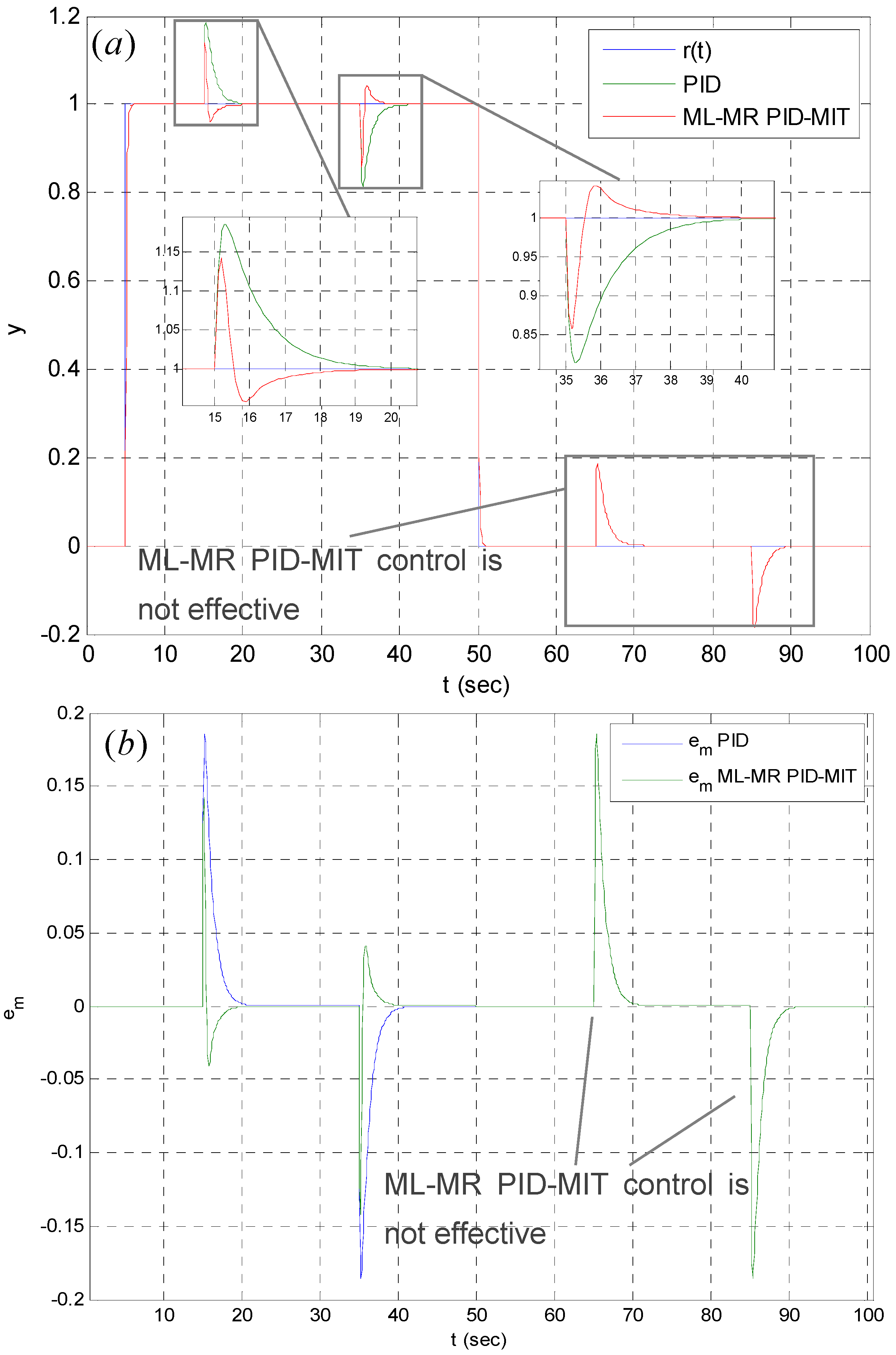
Figure 3 shows this effect for the ML-MR PID-MIT control structure design for control of the plant functions with zero time delay (
) and 0.3 s time delay (
) [
29]. The system responses in the figure demonstrate that the ML-MR PID-MIT control structure can significantly improve the disturbance rejection performance of classical PID control for zero delay systems. However, when the time delay of the plant increases, improvement in disturbance rejection control decreases.
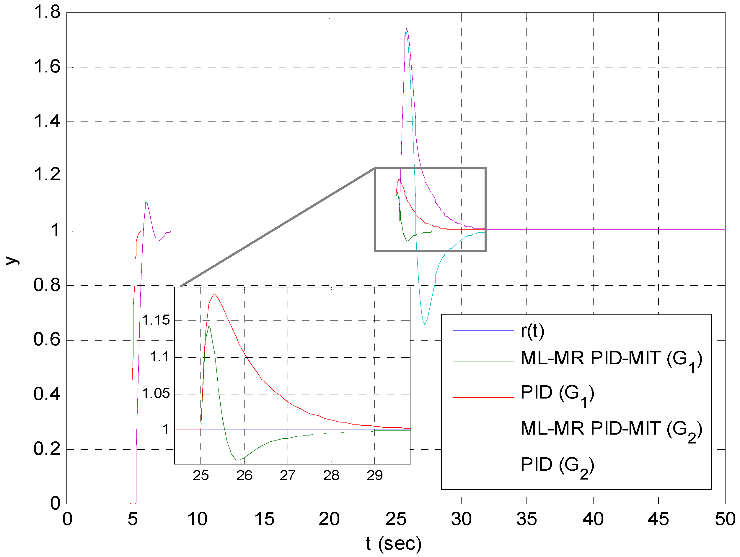
Secondly, due to multiplication terms and , the ML-MR PID-MIT control structure presents a nonlinear control characteristic. The origin of the nonlinearity in the adaptation gain is the nonlinear cost function, which involves the square of model error in Equation (3). This yields a nonlinear term . Therefore, ML-MR PID-MIT control can exhibit some characteristic properties that do not appear in linear control systems. A noteworthy property is that the time response of the PID-MIT control shows amplitude dependence. In the case of reference input , this results in ; in this case, the outer loop is not functional, so that in Equation (9). As the amplitude of the reference input signal grows, the amplitude of increases, and this effect indeed amplifies the model error due to the term of . Accordingly, this makes the MIT rule of the outer loop more sensitive to model errors and the system responds more effectively in cases where the model mismatches between reference model and control loops. To demonstrate this effect, an illustrative example for control of the plant function is carried out.
Figure 4 shows time response ML-MR PID-MIT control structure that is designed for plant function
[
29]. The learning rate
is set to −4, and the PID controller is configured to
,
, and
according to the Tavakoli–Tavakoli PID tuning rule in this simulation. When the amplitude of
moves to one (
), the ML-MR PID-MIT control structure becomes more effective and contributes to the disturbance rejection control performance of the inner loop (classical PID control loop). However, when the amplitude of
moves to zero (
), the ML-MR PID-MIT control structure is not functional, and its disturbance rejection control performance becomes the same as the disturbance rejection performance of the classical PID controller. The overlapping of time responses at set-point zero in the figure apparently confirms this effect.
3. Multi-Loop Model Reference PID-MIT with Controller Gain Modification (ML-MR PID-MIT-CGM): Adaptive RDR Adjustment for Dynamic Disturbance Rejection and the Linear Adaptation Rule
The disturbance rejection capacity of a closed loop control system can be expressed with the reference to disturbance ratio (RDR) spectrum, which presents a measure for the additive input disturbance rejection performance of a control system for each frequency component [
4,
30]. The analysis demonstrated that the RDR performance of a closed loop control system depends on the spectral power density of the controller function [
4]. The RDR spectrum of the PID controller is expressed in the form of [
4]:
The increase of low frequency RDR values improves the disturbance rejection control for low frequency and steady disturbance signals. An increase in high frequency RDR values improves the transient disturbance rejection performance. However, as mentioned previously, the tradeoff between disturbance rejection control and set-point control performance bounds the RDR performance of the closed loop PID control systems [
4]. A large increase in RDR values deteriorates the step response performance; this results in very high overshoots and consecutive ripples, which delay the convergence of the controlled system output to the set-point. Further increases in RDR values finally lead to instability of the control systems [
4]. Therefore, the unstable state of the closed loop control systems limits the improvement of their RDR performances. A solution for this problem is adaptive adjustment of RDR performance; RDR performance should be increased for disturbance incidents in the inner loop. In order to adjust the RDR performance of the PID control loop adaptively, a variable gain PID controller is proposed by multiplying the PID controller function with the adaptation coefficient
. This modified PID controller function allows adjustment of the DC gain of the classical PID controller by means of the coefficient
. The transfer function of this controller can be expressed as:
The RDR spectrum of this RDR-adjustable PID controller can be obtained as:
This expression of the RDR spectrum apparently shows that the proposed variable gain PID controller
allows modification of the RDR spectrum via adaptation gain
. This enables adaptive adjustment of the disturbance rejection performance of the inner loop by the outer loop. Since the gain
amplifies the control error inside the inner loop, the value of the adaptation gain
should be configured to remain positive, and hence is written by:
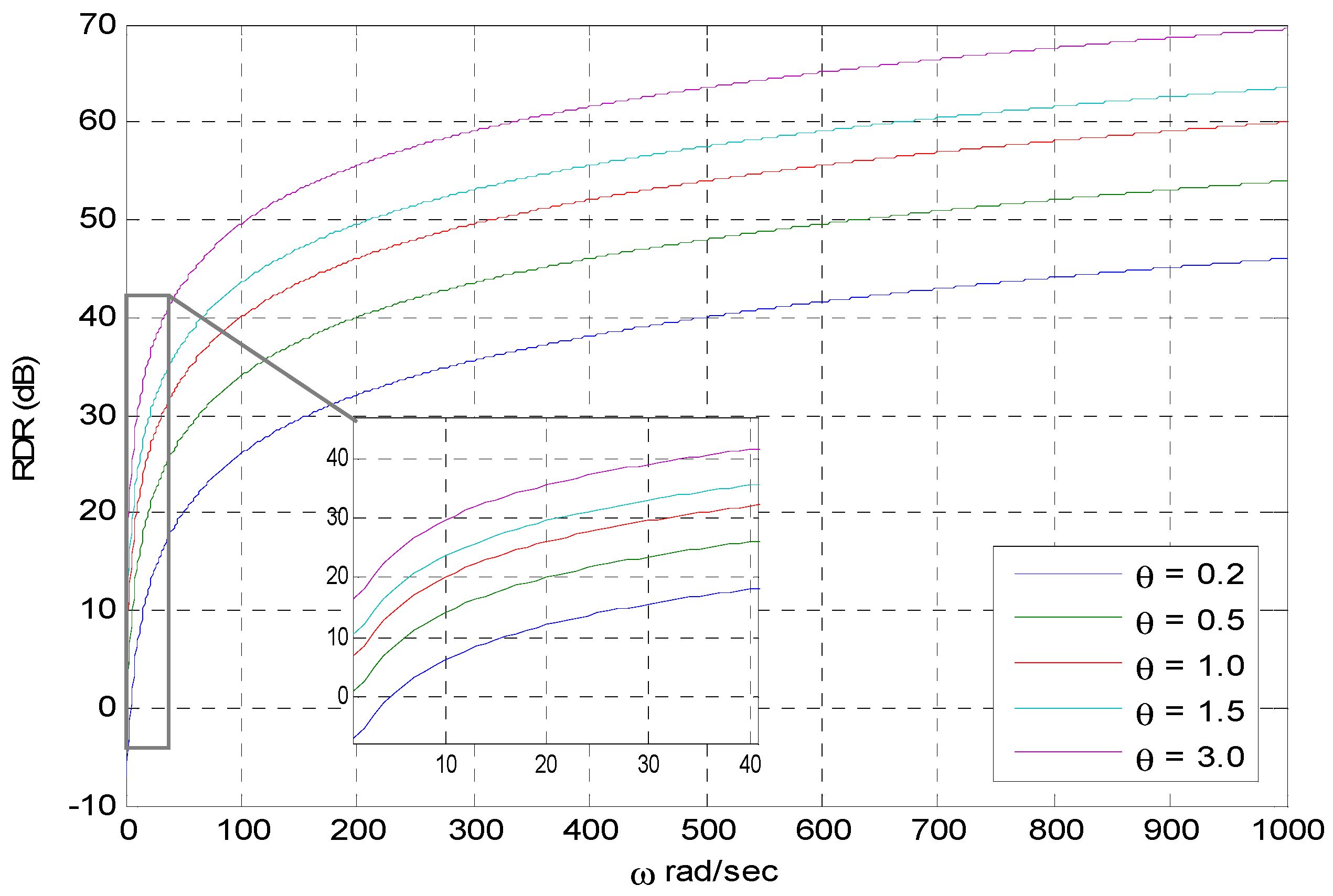
Figure 5 shows the RDR spectrum of the controller
for several values of the gain
. This figure reveals that the proposed variable gain PID controller
enables modification of the RDR spectrum via the gain
, and this asset allows adaptive adjustment of disturbance rejection performance in the control loop. For
, the
controller exhibits disturbance rejection performance equal to the performance of the classical PID controllers. When
, the disturbance rejection performance of
increases, as illustrated in the RDR spectrum in
Figure 5. It should be noted that the variable gain PID control may cause instability, particularly for time delay systems, because higher values of the gain
result in greater amplification of the integral gain, which may cause instability in the control systems as a consequence of accumulation of integral element control errors during the delay period of the system response. This limits the application domain of the proposed method to stable and almost-zero time delay plant functions.
The application steps for ML-MR PID-MIT with controller gain modification (ML-MR PID-MIT-CGM) for existing control loops can be given as follows:
Step 1: Obtain a transfer function model of an optimal control loop and use this transfer function as a reference model of the MRC loop ().
Step 2: Enclose the existing closed loop control system by the outer loop, as shown in
Figure 6. Apply the MIT rule for controller gain modification of the closed loop PID control system to adjust the RDR.
To show an application of the ML-MR PID-MIT-CGM control structure, an Automatic Voltage Regulator (AVR) control example is presented in this section.
Figure 7 shows a block diagram of the proposed ML-MR PID-MIT-CGM control structure for the AVR control example. The learning rate
is set to 10.
Bendjeghaba et al. implemented an improved harmony search algorithm for optimal tuning of closed loop PID control of an AVR model. The optimal PID controller was obtained by Bendjeghaba et al. in [
31] as:
We used this optimal PID controller for the AVR model in
Figure 7.
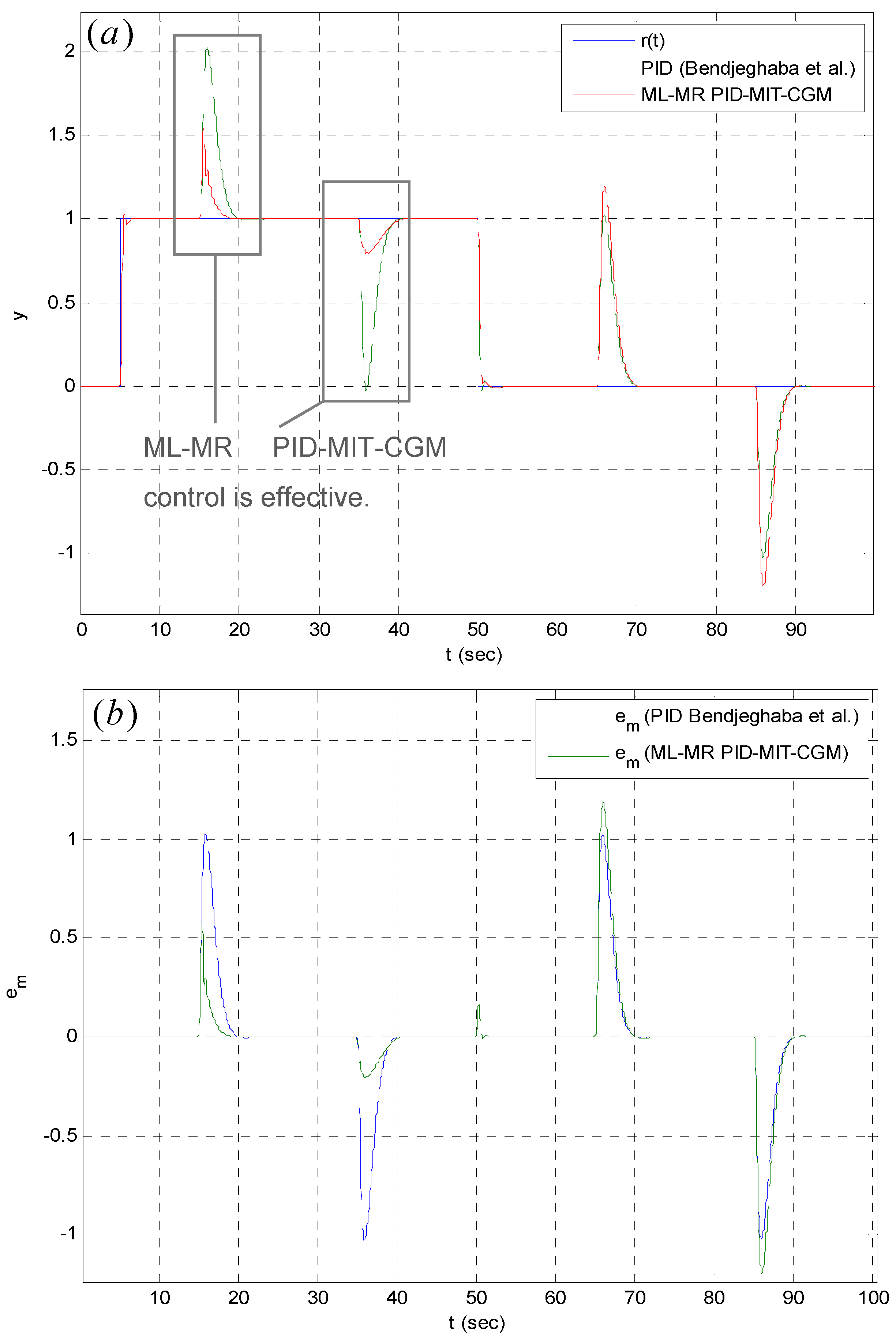
Figure 8a,b show responses of Bendjeghaba et al.’s optimal PID control loop and ML-MR PID-MIT-CGM control structure for square waveform input disturbances. The figure clearly shows disturbance rejection performance improvements for the ML-MR PID-MIT-CGM control at simulation times of 15 and 35 s, where the set-point is equal to 1. At these instances, the adaptation gain
of the outer loop actively responds to step-up and step-down disturbances, and it increases the RDR performance of the inner loop by increasing
, as illustrated in
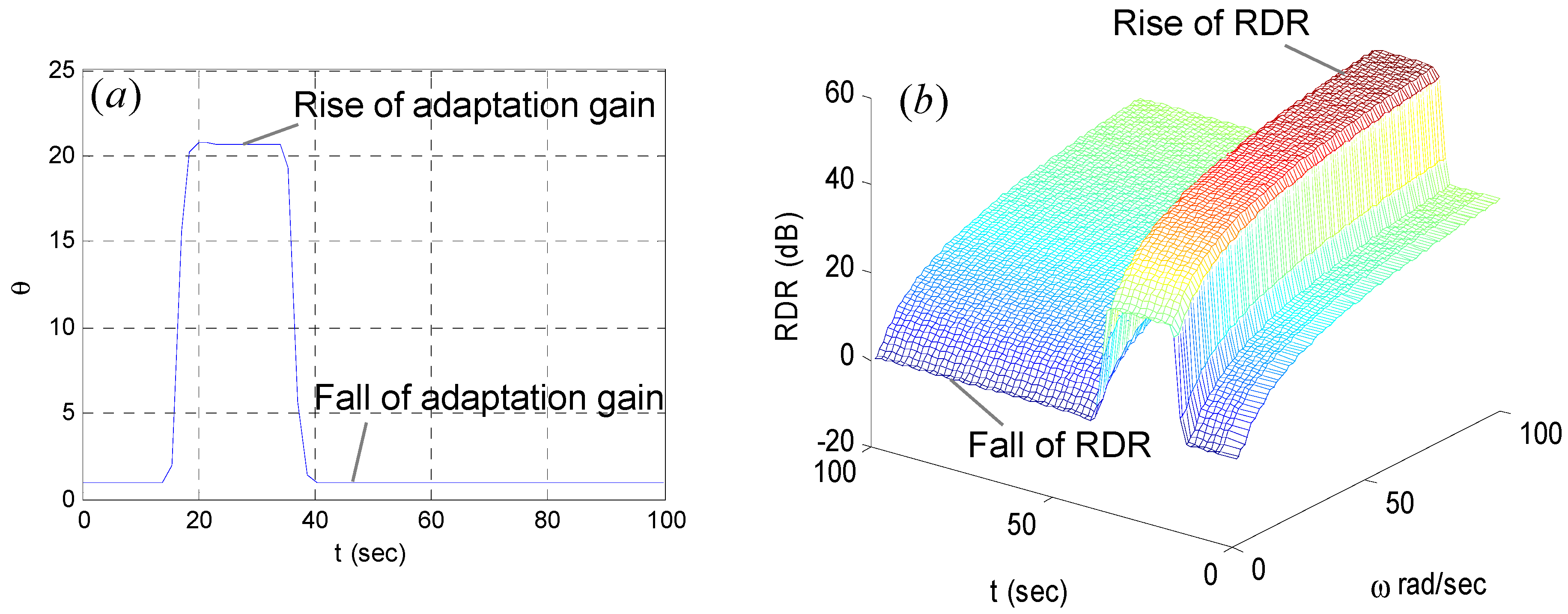
Figure 9. This effect provides a better disturbance rejection control than the classical PID control loop. Due to the amplitude dependence of the MIT rule, contributions of the ML-MR PID-MIT-CGM control to the disturbance rejection performance begin to vanish in the vicinity of the set-point 0. Consequently, the system can respond slightly better for step-up and step-down disturbances at the simulation times of 65 and 85 s compared to the optimal PID loop proposed by Bendjeghaba et al.
Figure 9 describes how ML-MR PID-MIT-CGM control responds to disturbance incidents. For a disturbance incident, the gain
increases, as shown in
Figure 9b. This results in an increase of PID coefficients, and accordingly an increase in the RDR rates in the spectrum, as shown in
Figure 9b. Therefore, the RDR performance of the optimal PID control loop of Bendjeghaba et al. is adaptively modified by adaptation gain
, while the disturbances affect the system response. This figure verifies an important asset of the proposed ML-MR PID-MIT-CGM control structure: It adaptively adjusts the disturbance rejection control performance and retains the set-point control performance of the optimal PID loops in absence of disturbance incidents. Thus, it overcomes the inherent shortcoming that is caused by the performance tradeoff between set-point control and disturbance rejection control. This property can significantly contribute to the practical robust control performance of classical control loops and can be viewed as an elegant solution for increasing the disturbance rejection performance without deteriorating the set-point performance of control systems. However, there will be a few drawbacks in the PID-MIT structures for linear control system applications. The nonlinearity of the MIT rule leads to dependence of disturbance rejection performance on the level of the set-point. Another drawback for linear control applications is that the performance of the PID-MIT-CGM control structure is very sensitive to the time delay of plants. A sufficiently large time delay may easily lead to instability in the systems.
As mentioned in the previous section, the MIT rule does not behave linearly due to the terms of
. To eliminate this nonlinearity and to make structural contributions to the PID control loop independent of the level of signal amplitudes, one can update the term
as
, where the constant
can be typically set to 1. This modification implies that the sensitivity derivative is constant and can be shown as
. Hence, Equation (16) is simplified to an integral operator and the adaptation gain can be written as:
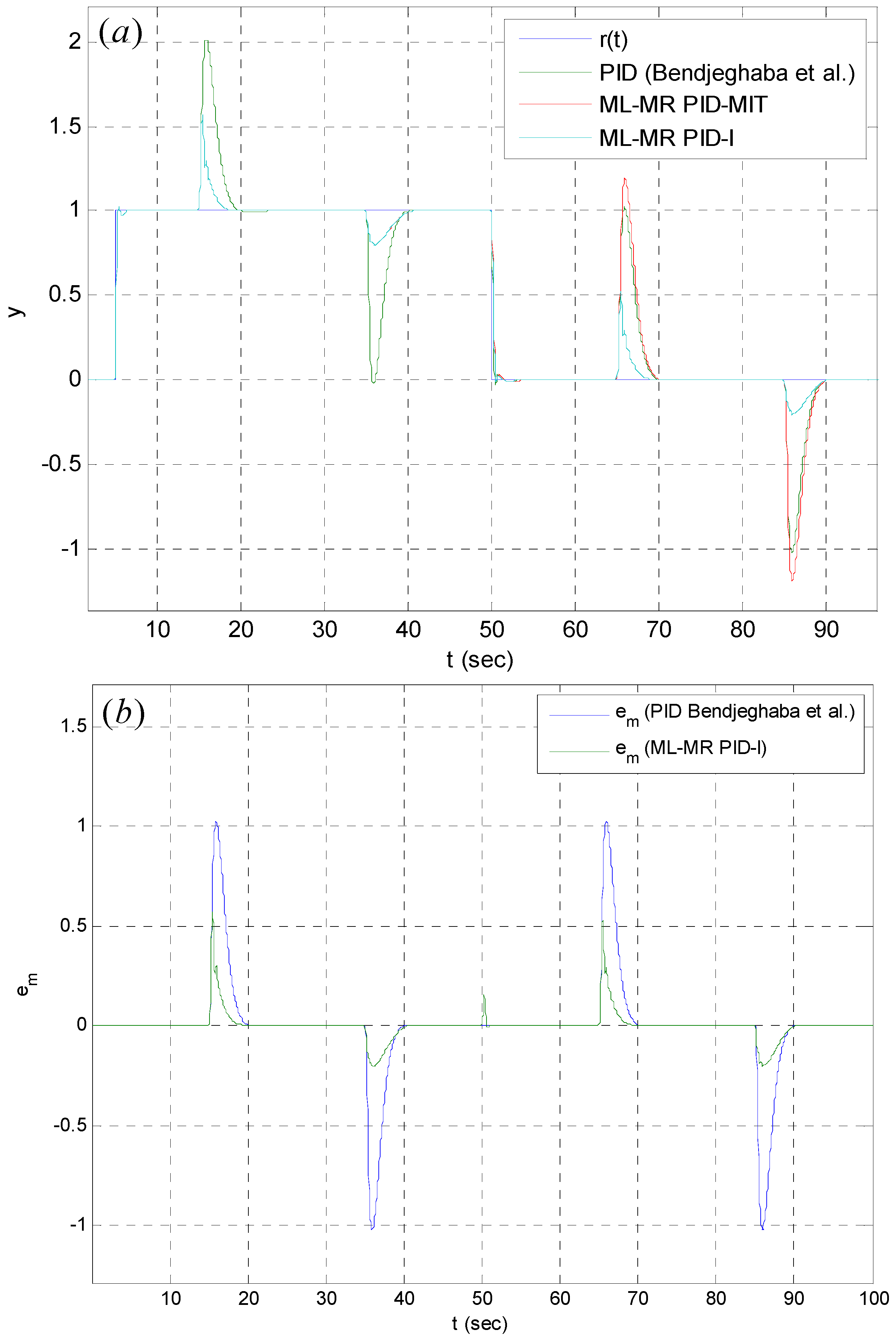
Using this modified adaptation gain—where Equation (18) replaces the MIT rule in Equation (16)—produces a new ML-MR control structure, which is called multi-loop model reference PID integral (ML-MR PID-I) control. The ML-MR PID-I control structure behaves linearly and improves the disturbance rejection performance independent of the reference input amplitude. Results in
Figure 10 demonstrate this effect. Although ML-MR PID-MIT-CGM is very effective around the unity set-point, its performance degrades at set-point 0, although it is slightly better than the optimal PID loop proposed by Bendjeghaba et al. However, ML-MR PID-I control presents the same performance as ML-MR PID-MIT control at the unity set-point and can maintain this performance improvement at set-point 0.
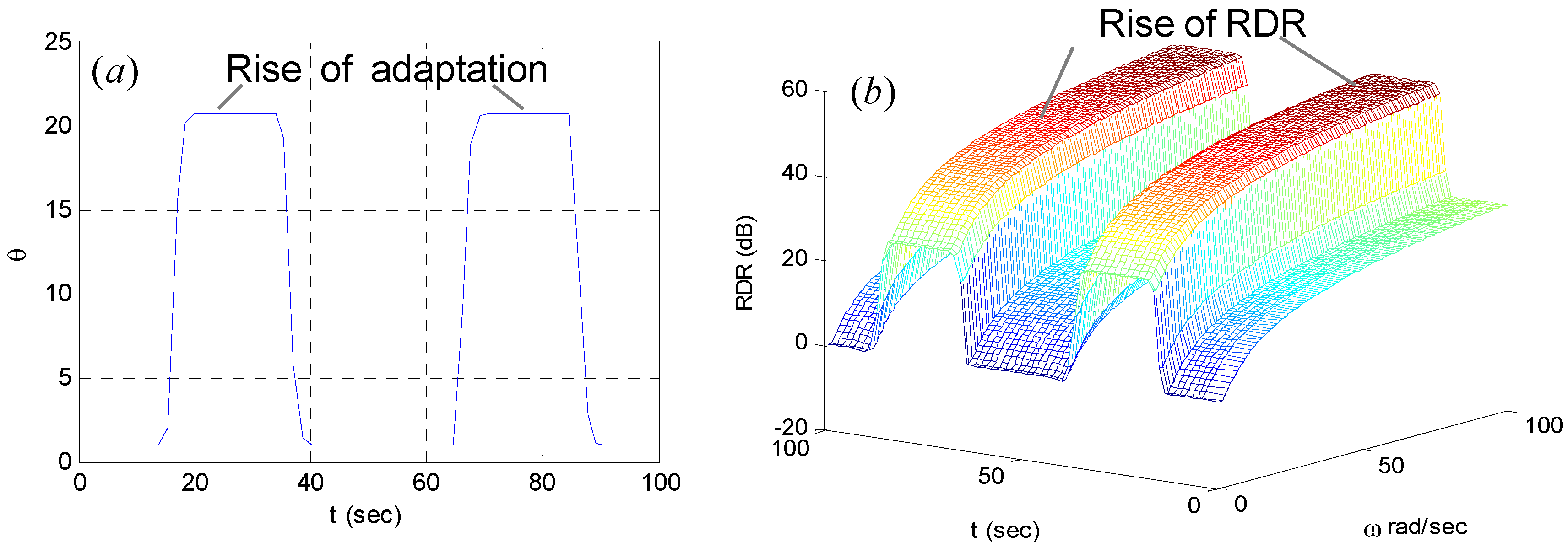
Figure 11 validates this effect by showing the adaptive adjustment of the RDR spectrum at set-point levels 1 and 0. As a consequence, for linear control systems with almost zero time delay, the proposed ML-MR PID-I control structure is capable of improving the disturbance rejection performance without deteriorating the set-point performance.
The simulation results verify the effectiveness of the ML-MR control loops by showing that the ML-MR control has a performance capacity beyond the typical disturbance rejection of classical single-loop control loops. This is a very useful property that improves the robust control performance in the case of disturbance interference to the control system. The ML-MR PID-MIT-CGM control structure is more preferable for set-point control of nonlinear systems, where linear ML-MR control structures are not an effective solution.
4. Multi-Loop Model Reference PID Internal Model (ML-MR PID-IM) Control Structure: Internal Model Linear Adaptation Rule
Internal model control (IMC) relies on a mathematical model of a plant or process, which is referred to as an internal model and performs the control law according to this internal model. It was reported that IMC can be an effective solution for disturbance rejection and model perturbation problems [
32]. In this section, we consider IMC to design a ML-MR control structure. Previously, an IMC-PID controller was proposed for improved disturbance rejection of time-delayed processes by using the reference model of the plant [
14]. IMC law can be designed by manipulating transfer function models of the control system. If the internal model is an accurate enough representation of the system, the derived control law in the s-domain becomes valid for the real system.
In this section, we assume that the internal model is the PID control loop (the inner loop) and design an internal model PID controller, such that the outer loop can perform the IMC for the inner loop. Let us consider the multi-loop control structure that is depicted in
Figure 1. To improve the disturbance rejection performance without influencing the control performance of the inner loop, the reference model, which is the internal model, is assumed to be the transfer function of the inner loop.
One can write the transfer function that involves the internal model controller loop
and the theoretical reference model
as:
Our design objective is to find an internal model controller
so that the whole system behaves the same as the theoretical reference model
, which represents an optimal design of the PID control loop. In order to achieve this objective, the transfer function condition
should be satisfied. By using
(Equation (19)), the transfer function condition becomes
. It is used in Equation (20) to satisfy the transfer function condition, which gives:
Then, the controller function
is written as:
By using Equation (19) in Equation (22), the
function is found:
where the
function is the open loop transfer function of the inner loop, which is expressed as
. In this form, the
function can be directly implementable. Application steps for existing control loops are summarized as follows:
Step 1: The transfer function model of an optimal control loop is obtained, and this transfer function is used as the reference model ().
Step 2: The optimal closed loop control system is enclosed by the outer loop, as shown in
Figure 12.
To demonstrate a possible application for the ML-MR PID-IM control, an example design for level control problem is presented. The plant model is an approximate model that represents the liquid level in the reboiler of the steam-heated distillation equipment [
14,
33]. The liquid level is controlled by adjusting the control valve on the steam line and the process model is given as
[
14,
33]. The optimal PID controller for improved disturbance rejection was given as [
33]:
The system model is unstable, and the controller function was obtained with negative coefficients. By considering Equation (23), the
function of the ML-MR PID-IM control structure is obtained as:
We implemented the ML-MR PID-IM control structure for this system, as shown in
Figure 13, and performed control simulations for square waveform input disturbance.
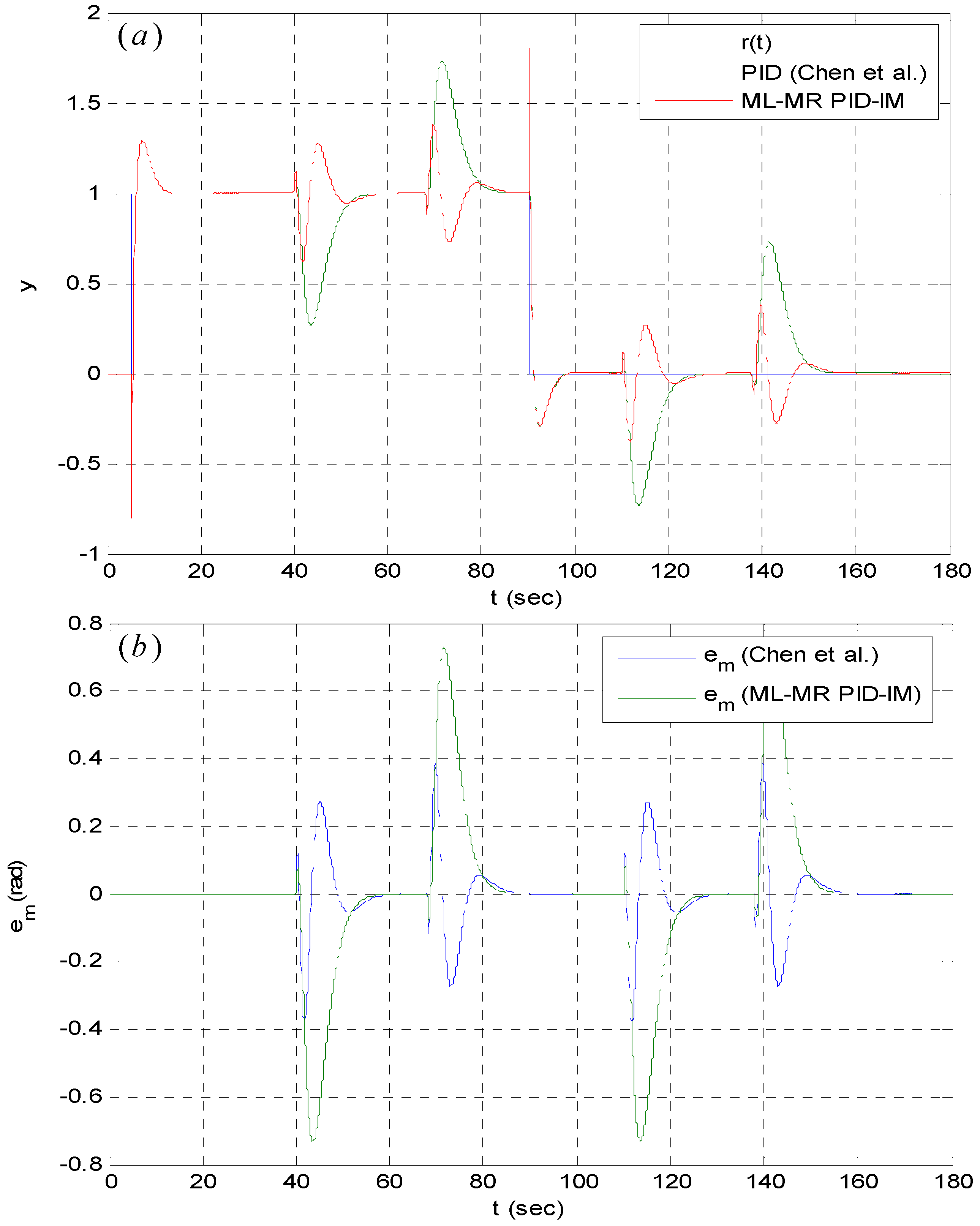
Figure 14 shows responses of the ML-MR PID-IM control structure and Chen et al.’s optimal PID control loop. Results in
Figure 14 clearly demonstrate that the ML-MR PID-IM control structure improves the disturbance rejection performance of Chen et al.’s optimal PID control loop without influencing its set-point performance. In the absence of disturbance, responses of the ML-MR PID-IM control structure overlap with responses of the optimal PID control loop. The set-point performance of the ML-MR PID-IM control is almost the same as the performance of the optimal PID control loop proposed by Chen et al. This is an important advantage for robust control performance so that the proposed ML-MR control structures can improve the disturbance rejection while maintaining the set-point performance of the existing PID control loops. A limitation of the ML-MR PID-IM control is that it is not an effective solution for large time delay plant dynamics and inaccurate plant models. High time delays can severely affect the performance of the ML-MR PID-IM control scheme.
6. Multi-Loop Model Reference PID-PID with Plant Function Adaptation (ML-MR PID-PID-PFA): Linear Adaptation Rule for Time-Delayed Systems
To obtain a linear adaptation rule, the MIT rule, which leads to nonlinearity, is changed to classical PID controller. ML-MR PID-PID-PFA control is implemented, as illustrated in
Figure 16.
The design steps of the ML-MR PID–PID-PFA control structure for a first order time delay plant in the form of can be carried out as follows.
Step 1: Identify the model of the plant function and take the reference model of the MRC loop as the plant function ().
Step 2: Enclose the MRC loop with the optimal closed PID controller loop, as shown in
Figure 16. Tavakoli-Tavakoli PID tuning rule, which is expressed by Equation (10), is used for the both PID controller functions.
To demonstrate the effectiveness of the ML-MR MIT-PID-PFA and ML-MR PID-PID-PFA control structures, we used them to enhance the first order plus deadtime plant model, which was given by Monje et al. [
34].
This plant function is a first order dynamical model of the Basic Process Rig 38–100 Feedback Unit (produced by Feedback Instruments Ltd) experimental platform [
34]. This system presents a 50 s time delay with a time constant of 433.33 s and is considered a large time delay process. Monje et al. designed an optimal fractional order PID (FOPID) controller for this system as follows:
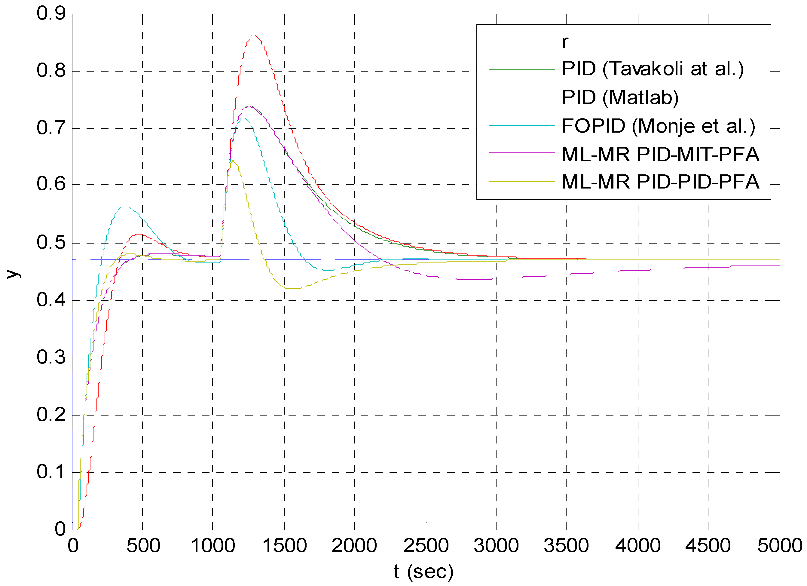
We implemented the ML-MR MIT-PID-PFA and ML-MR PID-PID-PFA control structures for this system by following the design steps given above. For control performance comparison purposes, we implemented a classical optimal PID control system with the Tavakoli–Tavakoli PID tuning rule (
,
,
), a classical optimal PID control loop with MATLAB optimal tuning (
,
,
), and an optimal FOPID control system with Monje et al.’s tuning rule. The set-point of this experimental system was originally 0.47 [
34] and a step disturbance with an amplitude of 0.47 at 1000 s was applied to the input of the plant model. The results of the control system simulations are shown in
Figure 17. The simulation results reveal that both the set-point and disturbance rejection performances of the ML-MR PID-PID-PFA structure re better than other controllers. The lowest overshoot and fastest settling results were achieved by the ML-MR PID-PID-PFA structure. It is noteworthy to observe that the control performance of the ML-MR PID-PID-PFA structure is superior to the optimal FOPID control system. This finding is a clear indication of the potential for multi-loop PID controllers to surpass the control performance of the FOPID controllers. The FOPID controllers have been considered as substitutes for classical PID control and have been extensively studied in the last decade, showing performance improvements of FOPID controllers over classical PID controllers. A major complication in practice for FOPID controllers is their realization complexity. Fractional order controllers can be implemented by using integer order models because near-ideal realization of fractional order derivatives and integral elements in digital systems is highly computationally expensive [
2]. Recently, analog circuit realizations of fractional order controllers have been shown, with results promising low-cost and low-complexity solutions for practical realization of FOPID controllers [
35,
36]. Recent works have shown the robust control performance improvement of MR-ML control structures with FOPID controllers [
25,
26], indicating an avenue for robust control system research.
It is useful to investigate the frequency dependence of disturbance rejection performance. For this purpose, the performances of the classical closed loop PID control structure and ML-MR PID-PID-PFA control structure were compared in the control problem of the Basic Process Rig 38–100 Feedback Unit experimental platform [
34] using sinusoidal waveform disturbance signals at several frequencies. The PID controller was tuned according to the ITAE design rule proposed by Tavakoli et al.
Table 1 shows the mean absolute error (MAE) of the control error signal (
) from simulations. For step disturbance, the ML-MR control structure reduces 50% the MAE of classical PID control system. In general, environmental disturbances are altered slowly and involve low frequency components. For very low frequency disturbance signals, the MAE of the ML-MR PID-PID-PFA control structure decreases down to 25% of the MAE of the classical PID control system. As the disturbance frequency increases, the MAE performance of the ML-MR PID-PID-PFA control structure equals the classical PID control structure.
Figure 18 shows some of the simulation results and confirms these findings.
In former studies, a ML-MR control structure using the MIT rule was experimentally verified for control of an experimental magnetic levitation system [
26] and control of an experimental electrical rotor [
28]. We conducted an experimental study to validate the contribution of the ML-MR PID-PID-PFA control structure to the disturbance rejection performance of classical PID control systems. A twin-rotor multi-input multi-output (MIMO) system (TRMS) is a popular rotor control test platform that is preferred for electrical rotor control experiments [
37,
38]. The TRMS is composed of two electrical rotors [
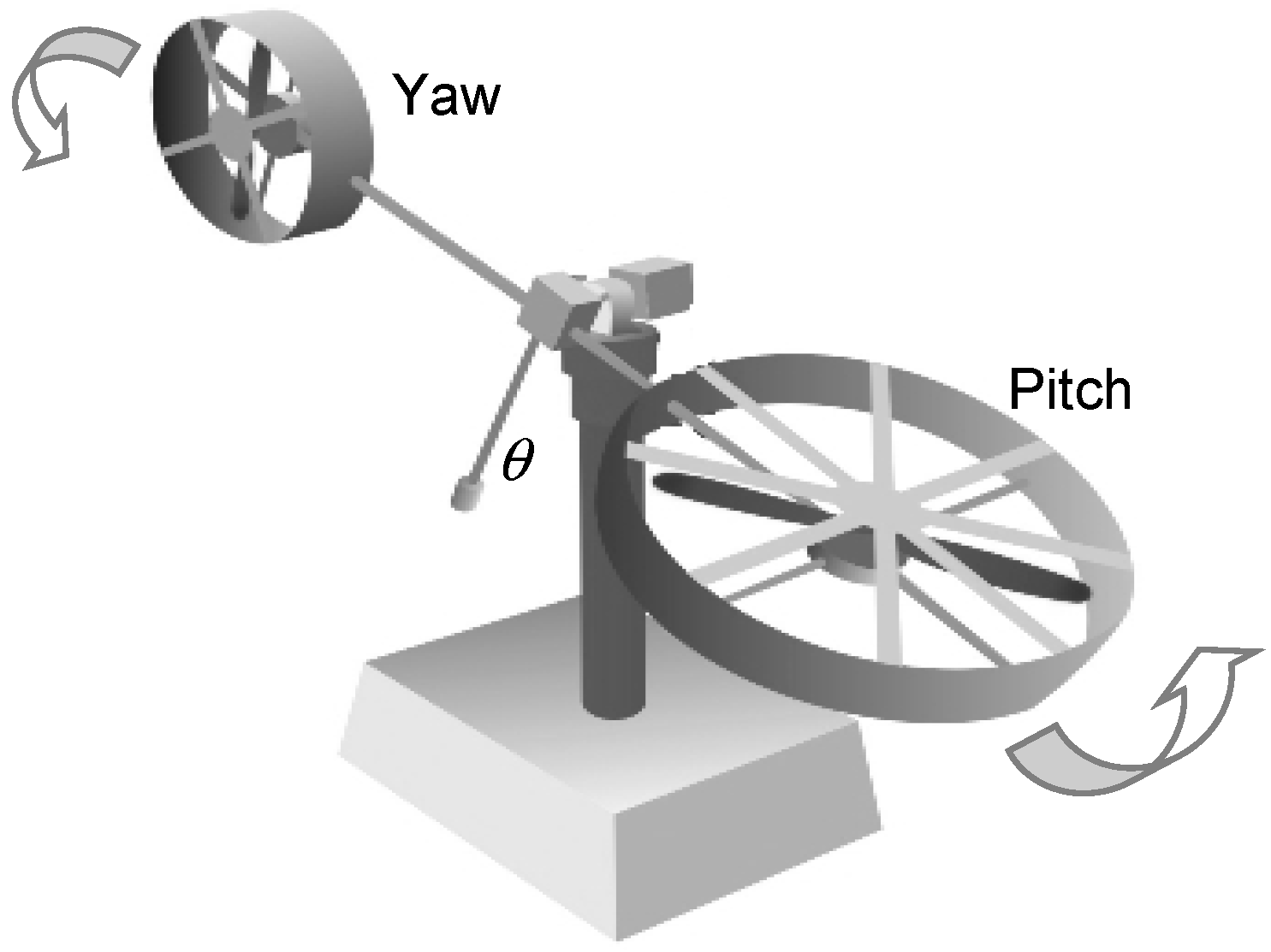
39]. These are pitch and yaw rotors, as illustrated in
Figure 19. The angles of the rotors are controlled by regulating the input voltages of the DC electric motors. This adjusts the rotational speed of the propellers so that the rotors can hover.
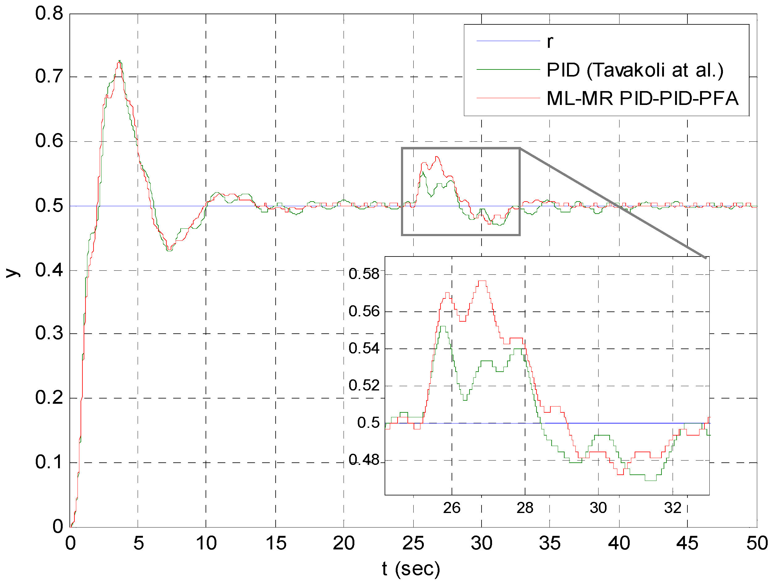
Figure 20 shows the experimental results. After settling the pitch angle to 0.5 rad, an input disturbance with a unit step waveform was applied at 25 s. One can observe that the step-point control performances of the classical PID controller and ML-MR PID-PID-PFA control structure are almost the same. The slight differences are mainly caused by internal system noise and limitations of the reference model in representing whole dynamics in the main rotor of the TRMS experimental setup. When disturbance is applied to the system, the response of ML-MR PID-PID-PFA control structure differs from the response of the PID controller and better rejects the disturbance at the system output, as shown in the figure.
One of major technical complications that was observed in the experimental study was the model mismatch problem in the real system. We used a nonlinear model of TRMS that is a good representation of experimental systems. However, inherent limitations of mathematical modeling and changes of operating conditions reduce the model consistency and lead to model mismatching problems. Since the response of reference model does not adequately match with the response of the real TRMS setup, the PID controller of the adaptation loop, which generates the adaptation gain , can cause instability in the system for the same PID controller coefficients for the control loop. This stability problem can be solved by retuning the PID controller to the adaptation loop.


