Designing the Uniform Stochastic Photomatrix Therapeutic Systems


1
Biochemistry and Molecular Biology Department, University of Arkansas for Medical Sciences, 4301 W. Markham St., Little Rock, AR 72205, USA
2
Department of Information Systems and Computer Science, Bauman Moscow State Technical University, 2nd Baumanskaya St., 5/1, 105005 Moscow, Russia
3
Winthrop P. Rockefeller Cancer Institute, University of Arkansas for Medical Sciences, 4301 W. Markham St., Little Rock, AR 72205, USA
*
Author to whom correspondence should be addressed.
Algorithms 2020, 13(2), 41; https://0-doi-org.brum.beds.ac.uk/10.3390/a13020041
Submission received: 13 December 2019
/
Revised: 5 February 2020
/
Accepted: 12 February 2020
/
Published: 18 February 2020
(This article belongs to the Special Issue Algorithms for Human-Computer Interaction)
Abstract
:Photomatrix therapeutic systems (PMTS) are widely used for the tasks of preventive, stimulating and rehabilitation medicine. They consist of low-intensity light-emitting diodes (LEDs) having the quasi-monochromatic irradiation properties. Depending on the LED matrix structures, PMTS are intended to be used for local and large areas of bio-objects. However, in the case of non-uniform irradiation of biological tissues, there is a risk of an inadequate physiological response to this type of exposure. The proposed approach considers a novel technique for designing this type of biomedical technical systems, which use the capabilities of stochastic algorithms for LED switching. As a result, the use of stochastic photomatrix systems based on the technology of uniform twisting generation of random variables significantly expands the possibilities of their medical application.
1. Introduction
The photomatrix therapeutic system (PMTS), in its generalized form, is a net of light-emitting diode (LED) irradiation sources on a dimensional plane, and the LEDs themselves are located in the nodes of this grid, which in turn is fixed by the given spatial dimensions [1,2,3,4,5,6]. The issues of designing PMTS medical devices have already been described, making it possible to combine three principal aspects: illumination and optical characteristics of LEDs, their spatial and geometric arrangement on the surface of matrix substrate, and also the parameters of photobiological influence on the body in the context of the given biomedical requirements [7,8,9,10,11,12,13].
Superbright LEDs possess quasi-monochromatic properties, i.e., relatively narrow spectral width of the irradiation range—up to several nanometers, depending on the central wavelength of the light source [14,15,16,17,18,19,20]. In certain medical tasks they could be considered as point laser sources, comparable with small laser diodes. Although the emission of LEDs does not satisfy such basic properties as coherence and polarization, which are inherent in laser irradiation, a huge amount of biomedical data indicate a close similarity between these two types of light sources. This is mainly due to the fact that when irradiating the skin of a biological object, the unique laser properties are largely leveled, starting from a depth at around three hundred microns from the skin surface [1,3,4,14,15,16,17,18].
In modern medical practice, phototherapy methods, including those based on superbright LEDs, have taken a strong place among the techniques of system-wide exposure to the human body [19,20,21,22,23,24]. In general, the basic principle of photobiological exposure is that a pronounced photoactivation occurs at the molecular, cellular, tissue, organ, and systemic levels in the bio-object. The main effects of phototherapy should be considered a systemic improvement in metabolism, as well as the normalization of blood flow components, for example, blood viscosity, microcirculation and rheology parameters, immunologic responses, and secondary regenerative processes, among others [21,22,23,24,25,26,27]. As a result, expressed therapeutic effects are achieved, such as biostimulatory, anti-inflammatory, analgesic, and decongestant effects, and many others.
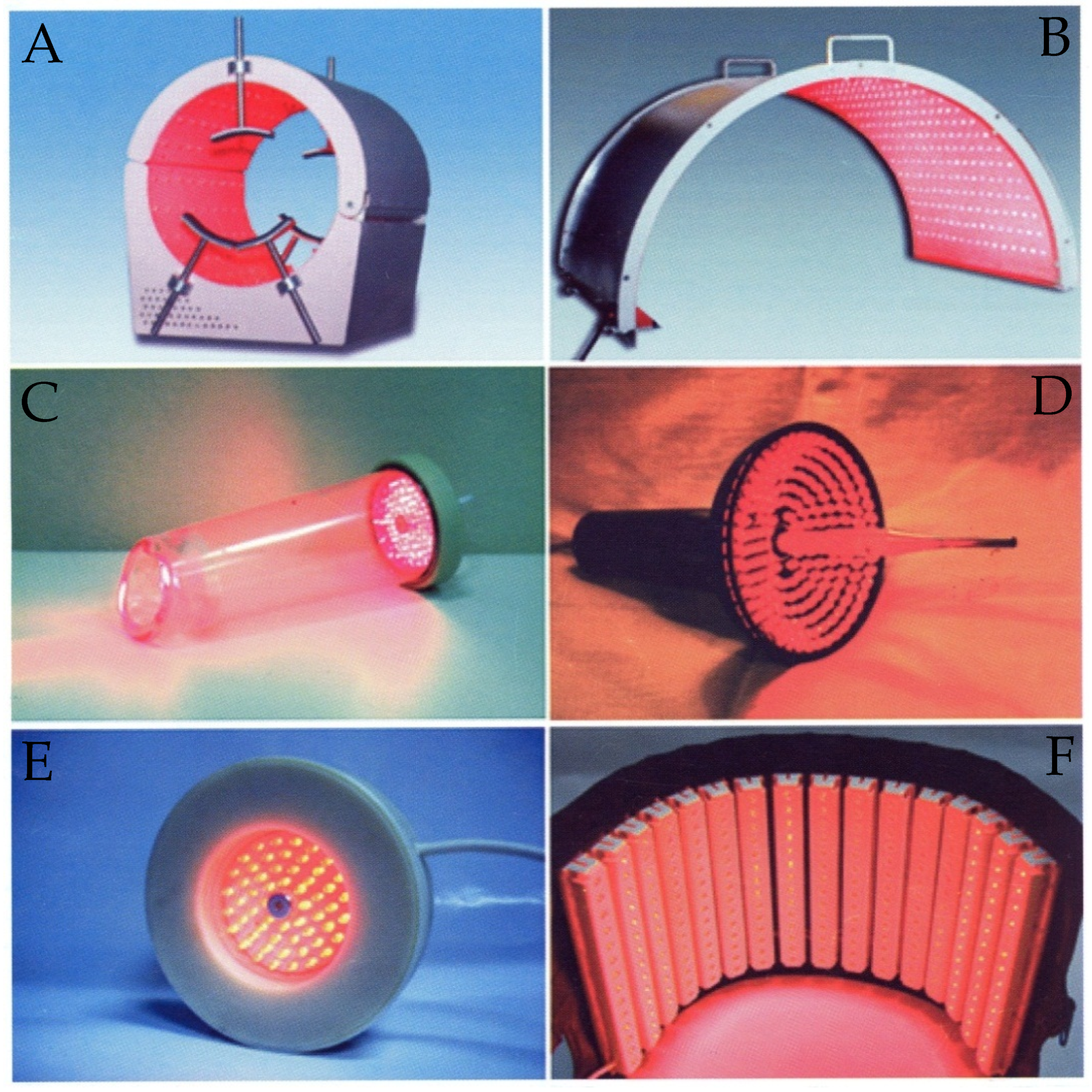
Several typical medical PMTS are presented in Figure 1. In particular, Figure 1A shows a cylindrical apparatus for photomatrix action on extremities of hands and feet, and Figure 1B presents a semicylindrical apparatus for the integral irradiation of extended skin surfaces, such as the abdomen or back. In addition to devices for the LED exposure alone, there are also combinations with other various sources of low-intensity physiotherapy. In particular, Figure 1C shows an apparatus that combines both LED irradiation and negative low-intensity pressure for the treatment of copulative dysfunction; Figure 1D displays a photo-ultrasound tool for treating the infected and purulent-necrotic wounds, which consists of a spherical segment of PMTS and a low-frequency ultrasonic waveguide; Figure 1E demonstrates a device combining LEDs of various wavelengths and a low-intensity magnetic field to affect various systems of the human body, for example, nervous, circulatory, musculoskeletal, etc., in order to enhance metabolic processes. In addition to the rigid frames in which the LEDs are fixed, there are also many PMTS based on flexible substrates, which provide a more accurate correspondence to the reliefs of biological tissues. Therefore, Figure 1F presents a semi-flexible construction of PMTS designed for various medical tasks based on LED phototherapy. In general, over thirty different types of PMTS are presently available on the market or known as laboratory prototypes.
The following operating modes of PMTS have been demonstrated [1,2,3,4,5,6,7,8,9,10,11,12,13]: constant, when all LEDs are on, but no modulation of irradiation is performed; blinking, where the LED sources are switched on at a specified frequency; blinking with pulse rate biosynchronization (based on pulse oximetry using a fingertip), in this case, the emission intensity of all LEDs is directly proportional to the volume of arterial blood supplying the vessels; looped modes of sequential single activation of each source or all LEDs lying on the same coordinate line; a variety of schematic modes such as ‘treadmill’ or specially designed modifiable ‘patterns’; modes of sequential or predetermined changes in the wavelengths of the LED irradiation (in the case of tunable sources); various stochastic modes for turning on the LEDs that are controlled using a connected random number generator; and others.
However, the stochastic modes for PMTS operation have not been sufficiently explored at present. Moreover, absolutely all known pseudo-random number generators, which are also used for biomedical technical systems, have a varying degree of uneven generation. In the case of PMTS, this means non-uniform generation of turning on the irradiation sources, i.e., the LEDs. This, in turn, can lead to some inadequate physiological responses of the body, at least at the biotissue level.
Moreover, in a worst-case scenario, such a non-uniform distribution of the modulation of the LED sources operation could be the reason for unpredictable reactions of the body. As a result, instead of low-intensity light stimulation, the physiological answer of the biological object may lead to unforeseen actions after such an unbalanced integral influence. In other words, an irregularly illuminated organism, i.e., somewhere unirradiated at all, and somewhere irradiated unnecessarily, can erroneously cause the compensatory mechanisms of patient’s biosystems.
Thus, the goal of this article is the study and creation of uniform stochastic modes for LED phototherapy that satisfy the conditions of uniform twister generation of light by point LED sources located on the PMTS surface.
2. Theory
The main advantage of the PMTS in comparison with other optical sources is the provision of the required irradiation intensity over the entire area of a sufficiently extended biological surface. However, as such, the spatial irradiation of a bio-object by a certain group of LEDs cannot be considered uniform if the LED sources are not located on the PMTS substrate in accordance with a strictly specified calculated location. Without this, irradiation of the body surface at different points of the biological object will occur with different and uncontrolled intensities.
Many scientific methods have been proposed in the research articles on the issue of ensuring the uniform irradiation of an extended object using a group of LED sources or LED matrices [28,29,30,31,32,33]. It should be noted that one of the promising modern areas in this field is the development of various lens solutions for LED systems [34,35,36,37]. However, despite this, the task of uniform irradiating using various LED schematics is still more than relevant.
Thus, let us initially consider here the theoretical aspects of the mathematical and engineering calculations of LED matrices, which allow designing the PMTS satisfying the properties of the spatial uniformity of the irradiation intensity over the entire surface of the body. In accordance with this, the geometrical dimensions and relief parameters of the biotissue as a basis determine the spatial formation of the PMTS substrate. The main parameters of the typical LED used in PMTS are the following:
- -
- wavelength of LED irradiation at maximum , nm;
- -
- half-width of irradiation spectrum , nm;
- -
- luminous intensity at given current through LED, mcd;
- -
- double aperture angle , deg;
- -
- general voltage and current characteristics;
- -
- dependence of the luminous intensity on the direct current through LED;
- -
- maximum permissible electrical features of LED;
- -
- physical dimensions for particular LED and total amount of them;
- -
- general geometrical sizes of PMTS and shape of matrix surface.
In the current case, particular for our tasks of biomedical application of PMTS, the following assumptions could be made:
- -
- LED irradiation is quasi-monochromatic;
- -
- each LED is considered to be a point source radiating within the dimensional aperture angle;
- -
- the wavelength of the LED irradiation belongs to visible and near-infrared ranges;
- -
- the optical axis of LED is normal to the inner surface of PMTS and to irradiated biotissue.
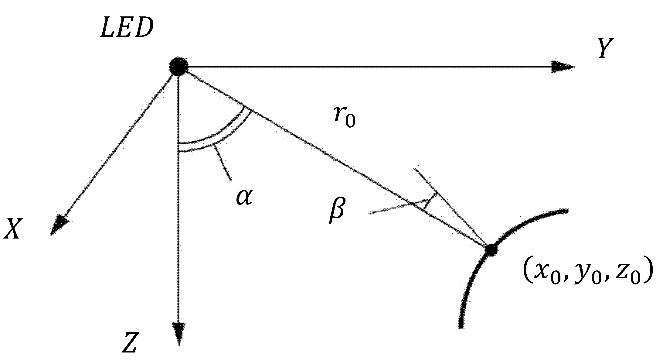
Now, let us determine the illuminance produced by a single LED. Consider orthogonal coordinates with LED at the origin of coordinates and Z-axis coinciding with the optical axis of the LED (i.e., the axis of the diode lens) (Figure 2).
In this case, the illuminance at some physical point of the irradiated surface is determined by the following equation:
where is derived from:
and angle is determined by:
Therefore, in the aforementioned equations, the key parameter is the luminous intensity of the single LED, then is the angle between the direction of irradiation and the optical axis of the LED, and is the angle between the direction of irradiation and the normal to the biological surface at a given point.
Equations for the angle depend on the frame shape of PMTS and the irradiated biotissue. Let us indicate here some typical cases of this interrelation:
- (1)
- flat PMTS irradiates a flat surface;
- (2)
- flat PMTS irradiates a cylindrical surface;
- (3)
- flat PMTS irradiates a spherical surface;
- (4)
- cylindrical PMTS irradiates a flat surface;
- (5)
- cylindrical PMTS irradiates a cylindrical surface;
- (6)
- cylindrical PMTS irradiates a spherical surface;
- (7)
- spherical PMTS irradiates a flat surface;
- (8)
- spherical PMTS irradiates a spherical surface.
For the first case mentioned above, angle is equal to angle , and so it is calculated as follows:
For the 2nd and 5th cases, the realization of angle is in the following form:
where and are derived from these equations:
In this case, for some spatial point Q, its coordinate reference will be determined by the expressions , and then , and will look as follows:
where the term c corresponds to the designation of the cylinder; if , then in this case and .
For the 3rd, 6th and 8th cases, the realization of angle is based on the same Formulas (5), (6) and (7); however, for some spatial point Q its coordinate reference will be determined by other expressions: , then by Formula (8), and will look as follows:
If , then in this case, and , where the term s corresponds to the designation of the sphere; next, if , then in this case and .
For the 4th case, the determination of angle will take the following form:
where is the angle between the Z-axis and the optical axis of the LED.
For the 8th case the determination of angle will look almost the same as the previous one; however, because of the spherical surface, the addition of the iteration step i is required:
In the simplest case, the luminous intensity of the single LED has the following form of dependence:
To calculate the illuminance resulting from a flat LED matrix, for example, at a point K lying on the optical axis of one of the diode sources, the following equation could be used:
where 2d is the distance between the adjacent LED point sources, and lo is derived trigonometrically as (Figure 3).
The first term of Series (13) describes the LED irradiation nearest to the point K. As the distance from the irradiating surface increases, new terms occur in the series due to obvious overlapping of light beams. This equation shows that theoretical determination of illuminance at an arbitrary point requires complicated calculations and unjustified simplifications. It is more appropriate to determine the LED light distribution over a surface of a certain type generated by one of the aforementioned types of PMTS or combinations of them. Also, it is better to assume that the shape of the irradiated biotissue can be approximated with a flat, cylindrical, or spherical surface. As a result, due to such assumptions, the general task of calculating the LED intensity created by the matrix structure can be divided into several special cases.
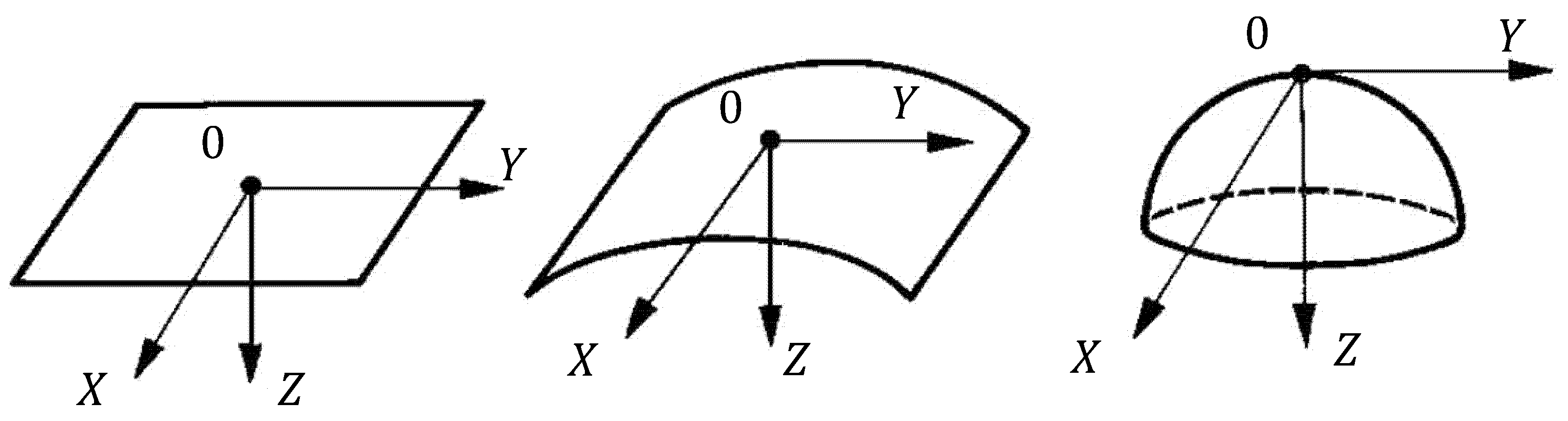
The illuminance at each point of the irradiated surface is calculated as the summarization of illuminances produced by each LED. In the process of calculation of the contribution of each LED the coordinate system is translated so that the origin of coordinates coincides with the LED under consideration, whereas the Z-axis is directed along the optical axis of the diode source (in the direction of light distribution). Thus, if coordinates of the point K in the new coordinate system are determined, then the illuminance is calculated using Formulas (1), (2) and (3). Such a basic coordinate system was selected to simplify the specification of parameters of the irradiated surface. Now, based on all of the aforementioned assumptions, let us consider several main methods of illuminance calculation produced by PMTS of various types.
Flat PMTS (Figure 4, left). For the flat type of PMTS the calculation begins from the upper left LED. In this case, the coordinates of the irradiated point are:
where dx and dy are the distances between adjacent LEDs along the X- and Y-axes of the basic coordinate system, respectively; Nx and Ny represent the numbers of LEDs along these axes.
The illuminance is calculated sequentially for LED rows parallel to the X-axis. As the coordinate system is translated along the X-axis, the coordinates are transformed as follows:
Furthermore, as the coordinate system is translated along the Y-axis, the following transformation of coordinates is used as well:
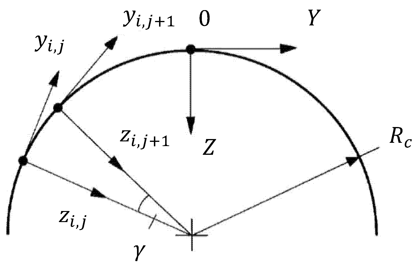
Cylindrical PMTS (Figure 4, center; Figure 5). Prior to the calculations of the cylindrical type of PMTS, the following parameters have to be specified: quantities and of LEDs along the generating line and the arc of the cylinder, respectively; distance between adjacent LEDs along the generating line; angle between adjacent LEDs lying on the same arc; PMTS cylindrical radius . At the beginning of the calculation, the coordinates of the irradiated point are:
where the angle for a non-closed cylinder is determined by the following equation:
For a completed cylinder of PMTS the angle if there are diode sources on the X-axis of the basic coordinate system; if there are no LEDs, then .
The illuminance is calculated sequentially for LED rows parallel to the generating line. As the coordinate system is translated along the generating line, the coordinates are transformed as follows:
In the next iteration, as the coordinate system is translated along the arc, the following transformation of coordinates is used:
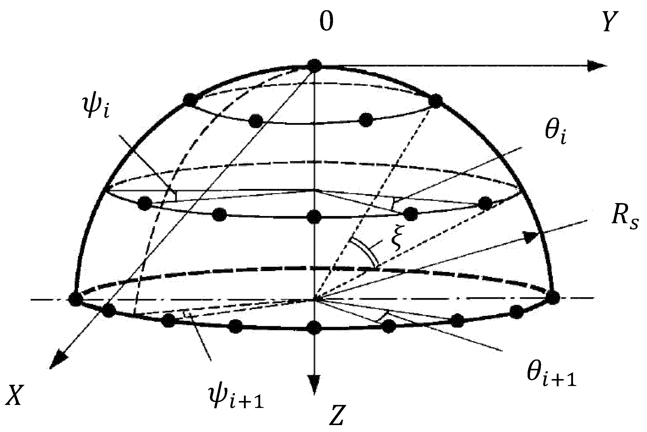
Spherical PMTS (Figure 4, right; Figure 6). This type of PMTS substrate is the most complex of all three cases, since its calculation depends on many related variables. The following parameters should be assigned for the spherical PMTS: radius of the sphere; number of parallel circles constituted by LEDs (a single diode source lying in the origin of coordinates); angle between parallel circles; angle between adjacent LEDs on the i-th parallel circle (, where is the number of LEDs on the i-th parallel circle); angular displacement between i-th and previous parallel circles, accordingly.
In the calculation of illuminance produced by a spherical PMTS, the coordinate system is translated in the following manner: first, the illuminance produced by the LED lying in the origin of the basic coordinate system is determined. Then, the coordinate system is translated to the first parallel circle and rotated by an angle ; then it is translated to the second parallel circle and rotated by an angle (it is assumed that ); then by an angle , and so on. Thus, the total illuminance will be obtained. As the coordinate system is translated from one parallel circle to another, the following transformation of coordinates is used:
Translation of the coordinate system along each parallel circle is performed clockwise when looking in the direction opposite to the Z-axis of the basic coordinates. The following alteration is used for translating the coordinate system along a parallel circle:
where is the angle between the axes and ; is the angle between the axes and ; , , , and are determined trigonometrically:
Next, after all the aforementioned assignments, it is time to introduce the rotation matrices used for calculation when transferring the coordinate system. These are determined by the following mathematical forms:
In the case when in these matrices , then the original Expression (22) used to move the coordinate system can be represented as the following transformation:
Thus, after transitions to the i-th parallel circle from the previous one the first step is the moving along with an angular displacement between those parallels, and only after that will one by one calculation take place for the value of angle between adjacent LEDs of spherical PMTS.
As a result, using the sequential transformations described above, the illuminance of the biotissues can be calculated for three main types of PMTS. At the same time, more complicated biological surfaces may be considered as a combination for these three PMTS types, and so the illuminance in this case can be calculated as well.
As noted at the beginning of this section, one of the main advantages of the PMTS over all other light sources is the integral spatial irradiation of extended biological surfaces having any skin relief. The methodology proposed above makes it possible to create a PMTS in which the LED sources are not located unsystematically or by chance, but in a certain order in accordance with the mathematical and engineering calculation algorithm. Thus, by strictly following the spatial mathematical model for calculating the placement of each LED, it will be possible to create such PMTS that will completely satisfy the properties of absolute uniform irradiation of the body surface with the same intensity over the entire irradiated area.
Furthermore, it should be emphasized that the algorithm proposed above describes how to create uniform spatial illuminance, which is true for a constant mode of the LED irradiation. However, this mode of PMTS operation is only the initial basic mode; all other regimes that were indicated in the Introduction section of this article are pulse-generated. The most complex of them is the stochastic mode, the implementation of which is not a trivial task, and thus has still not been fully solved in LED phototherapy. The questions regarding this issue are considered in the next sections.
3. Construction and Results
3.1. Features of Standard Programmable Tools
Usually, the control of complex modes of switching on LED elements is carried out using microcontrollers [1,14,17,18]. At the same time, the microcontroller itself is supplemented with special technical tools, i.e., it is almost an analogue of a computer, but with limited and specific capabilities. The assigned functioning of the microcontroller is determined by the internal software, which forms the irradiation modes of the LEDs both in time and in intensity. One of the popular programming languages for modern microcontrollers is the classical C language in different dialects.
Let us start from the question of uniform randomness, which is an important special case of the general concept of stochastic phenomena in probability theory, mathematical statistics and the theory of random processes [38,39,40,41,42,43,44,45]. Particularly for the current issue, i.e., in case of PMTS influence on biological tissue, this means an accurate understanding of the uniform operation of randomly turned on LEDs. The term ‘uniform random variables’ means that in the allotted time, all the exposure elements (LEDs or their analogues) are switched on precisely the same number of times [46,47,48,49,50,51]. Thus, it should be started with this, i.e., by checking the ability of standard tools to ensure the uniform generation of irradiation from point light sources.
The matrix of the Descartes plane U × V contains cells along the U orthogonal axis and cells along the V one. Thus, the matrix contains cells in total; in each of them, only one LED is located. The case of the arrangement of several point sources of light in one cell will not be considered here, since it is almost additively reduced to single-point emitters in the mathematical sense. Therefore, let us take as a basis the fact that, physically, the matrix accommodates M elements of LEDs located on a two-dimensional plane.
Furthermore, let us pay attention to an elementary but complete period of time, during which all LEDs must be turned on in a random sequence. The illuminance time of one LED is designated as τ. Therefore, the time interval of the full glow of all the LEDs in the matrix is . The minimum completeness of activation of the emitters means that they all turn on exactly once. In accordance with this, the potentials of coordinates assigned with the number of LEDs to be switched on and calculated from these coordinates are independently provided along the grid of LEDs. These coordinates uniquely correspond to the coordinates of the matrix cells . Random enumeration of these cells is a mathematical model of a stochastic emitting process by LED.
Based on principles described above, the following issue needs to be considered for the current task. Could the uncontrolled independent modeling of coordinates be accepted as a sufficient condition for the construction of LED matrices? We will demonstrate that such a technology produces poor quality results; after that, we will also show and discuss the proposed option in which the result of absolutely uniform distribution of the LED irradiation can be obtained.
Therefore, to find the answer to this question, let us take the standard function Random (), which comes as a generator of random variables together with other tools of C language. As an example, let us take the matrix plane having a size of cells, which accordingly consists of 64 LEDs. In reality, the number of cells can reach several hundred or even more. To demonstrate the result of the simulation, the code DMP0101 in C# dialect of Microsoft Visual Studio is given below.
        namespace DMP0101
        { class cDMP0101
         { static void Main(string[[] args)
          { Random GU = new Random();
           Random GV = new Random();
           int N = 8;      // length of sequences U и V
           Console.WriteLine("N = {0}", N);
           int[[] U = new int[N];       // U sequence
           int[[] V = new int[N];       // V sequence
           int[[,] A = new int[N, N];     // result matrix
           for (int i = 0; i < N; i++)
            for (int j = 0; j < N; j++) A[i, j] = 0;
            for (int i = 0; i < N; i++)   // one of the axes
            {  Console.Write("i = {0,3} | ", i);
             for (int j = 0; j < N; j++)   // another axis
             {  int u = GU.Next(N);    // random value u
              U[j] = u;       // random sequence U
              int v = GV.Next(4*N) % N;  // random value v
              V[j] = v;       // random sequence V
              A[u, v]++;  // <u,v> point generation counter
            }
            Console.Write("U = ");
            for (int m = 0; m < N; m++)
             Console.Write("{0,4}", U[m]);
            Console.WriteLine();
            Console.Write("   | V = ");
            for (int m = 0; m < N; m++)
             Console.Write("{0,4}", V[m]);
            Console.WriteLine();
           }
           Console.WriteLine("Matrix A");
           for (int i = 0; i < N; i++)
           {  for (int j = 0; j < N; j++)
             Console.Write("{0,4}", A[i, j]);
            Console.WriteLine();
           }
           Console.ReadKey();      // result viewing
          }
         }
        }
After launching the DMP0101 program, the following printout may appear, since Random () can provide new of generation results at any time.
        N = 8
        i = 0 | U = 5 0 2 3 2 1 6 4
          | V = 6 0 5 5 3 5 3 3
        i = 1 | U = 1 3 6 0 1 2 3 3
          | V = 2 6 6 7 2 1 6 1
        i = 2 | U = 2 0 4 0 5 1 3 5
          | V = 2 1 5 1 5 0 4 1
        i = 3 | U = 2 6 0 3 2 1 6 0
          | V = 0 1 1 1 3 6 4 5
        i = 4 | U = 2 7 0 1 0 1 7 1
          | V = 0 0 7 1 7 3 7 7
        i = 5 | U = 5 0 4 2 3 6 1 3
          | V = 6 1 1 5 0 6 7 6
        i = 6 | U = 3 3 2 1 5 0 3 3
          | V = 6 3 6 5 5 3 6 5
        i = 7 | U = 5 5 0 4 0 3 1 7
          | V = 4 4 5 2 4 2 7 3
        Matrix A
        1 4 0 1 1 2 0 3
        1 1 2 1 0 2 1 3
        2 1 1 2 0 2 1 0
        1 2 1 1 1 2 5 0
        0 1 1 1 0 1 0 0
        0 1 0 0 2 2 2 0
        0 1 0 1 1 0 2 0
        1 0 0 1 0 0 0 1
The output of the printed sequences created by generator GU from the above program shows that starting from the first generation, the sequence string U = { 5 0 2 3 2 1 6 4 } demonstrates the repetition of random variable 2. This simple example indicates that frequencies of the matrix cells are not uniform, since some cells are activated several times. Specifically, in this case, one of the variables appears with a frequency of more than one. Thus, the analysis of the printout demonstrates that the standard generator Random () does not provide the proper quality of uniform stochastic activation of the LED sources of PMTS.
Currently, there are many generators available for the generation of variables, and all of them have different degrees of uniformity. For example, generator Random () demonstrates a level of uniformity which does not exceed 30%. This means that on the assigned diapason of variables, only 30% of them are distributed uniformly without repeated or skipped elements. Another well-known Mersenne twister generator MT19937 [52] shows a fairly high degree of uniformity, which is about 70%. At the same time, the twister generator nsDeonYuliTwist32D [48] has absolute complete uniformity in the range of random variables with w bit length.
Let us further test the generator nsDeonYuliTwist32D for its applicability for the construction of stochastic PMTS. It fully satisfies the properties of non-repeating and non-skipping of the generated elements. Below is the program code DMP0102 for the independent testing of generation quality, which is especially designed for the aforementioned task. The idea of this program fully coincides with the code DMP0101, but the realization is implemented using the complete uniform twister generator nsDeonYuliTwist32D instead of the standard Random () one. Let us emphasize here once again that generator Random () a priori cannot create sequences without the repetition or skipping of the elements. This is tantamount to a switched off state or a set of repeated switched LEDs on conditions.
        using nsDeonYuliTwist32D;    // twister uniform generator
        namespace DMP0102
        { class cDMP0102
         { static void Main(string[[] args)
          { uint w = 3;        // number bit length
           cDeonYuliTwist32D GU = new cDeonYuliTwist32D();
           GU.x0 = 1;       // U sequence beginning
           GU.w = w;         // number bit length
           GU.Start();        // GU generator start
           cDeonYuliTwist32D GV = new cDeonYuliTwist32D();
           GV.x0 = 4;       // V sequence beginning
           GV.w = w;         // number bit length
           GV.Start();        // GV generator start
           int N = 1 << (int)w;   // U and V sequences length
           Console.WriteLine("w = {0}  N = {1}", w, N);
           uint[[] U = new uint[N];      // U sequence
           uint[[] V = new uint[N];      // V sequence
           int[[,] A = new int[N, N];     // result matrix
           for (int i = 0; i < N; i++)
            for (int j = 0; j < N; j++) A[i, j] = 0;
           for (int i = 0; i < N; i++)   // one of the axis
           {  Console.Write("i = {0,3} | ", i);
            for (int j = 0; j < N; j++)   // another axis
            {  uint u = GU.Next();    // random value u
             U[j] = u;       // random sequence U
             uint v = GV.Next();    // random value v
             V[j] = v;       // random sequence V
             A[u, v]++;  // <u,v> point generation counter
            }
            Console.Write("U = ");
            or (int m = 0; m < N; m++)
             Console.Write("{0,4}", U[m]);
            Console.WriteLine();
            Console.Write("   | V = ");
            for (int m = 0; m < N; m++)
             Console.Write("{0,4}", V[m]);
            Console.WriteLine();
           }
           Console.WriteLine("Matrix A");
           for (int i = 0; i < N; i++)
           { for (int j = 0; j < N; j++)
             Console.Write("{0,4}", A[i, j]);
            Console.WriteLine();
           }
           Console.ReadKey();       // result viewing
          }
         }
        }
After starting the DMP0102 program, the following result appears on the monitor.
        w = 3 N = 8
        i = 0 | U = 1 6 7 4 5 2 3 0
          | V = 4 5 2 3 0 1 6 7
        i = 1 | U = 3 5 7 1 2 4 6 0
          | V = 1 2 4 6 0 3 5 7
        i = 2 | U = 7 3 6 2 5 1 4 0
          | V = 2 5 1 4 0 7 3 6
        i = 3 | U = 6 7 4 5 2 3 0 1
          | V = 5 2 3 0 1 6 7 4
        i = 4 | U = 5 7 1 2 4 6 0 3
          | V = 2 4 6 0 3 5 7 1
        i = 5 | U = 3 6 2 5 1 4 0 7
          | V = 5 1 4 0 7 3 6 2
        i = 6 | U = 7 4 5 2 3 0 1 6
          | V = 2 3 0 1 6 7 4 5
        i = 7 | U = 7 1 2 4 6 0 3 5
          | V = 4 6 0 3 5 7 1 2
        Matrix A
        0 0 0 0 0 0 2 6
        0 0 0 0 3 0 3 2
        3 3 0 0 2 0 0 0
        0 3 0 0 0 2 3 0
        0 0 0 8 0 0 0 0
        5 0 3 0 0 0 0 0
        0 2 0 0 0 6 0 0
        0 0 5 0 3 0 0 0
A direct check of the sequences U and V in each iteration over the index i shows their absolutely complete uniformity, i.e., sequences do not have skipping or repetition of random variables. However, the presence in matrix A of cells with values different from the number 1 means that the independent generation of the coordinates of random points on a plane does not provide a uniform distribution of these points on a grid of the discrete plane. Some points are absent altogether (values 0), others are present several times (values > 1). Therefore, following only the property of independent complete uniform generation of the coordinates of the matrix cells is not sufficient for the formation of uniform stochastic PMTS.
3.2. Features of Designing the Stochastic Programmable Tools
In the previous subsection, it was found that to create a uniform random plane, the independent generation of random variables along the axes of the Descartes coordinates in the photomatrix is not sufficient. In this case, the effect of an algorithmic dependence of the generated sequences of random variables may occur. Thus, let us indicate below the concept of a random plane.
Usually, in analytical geometry, a random arrangement of a plane in three-dimensional space is understood to mean a variation of its equation Ax + By + Cz + D = 0 with respect to the coefficients A, B, C and D. However, this definition is suitable only for the geometric arrangement of the plane [53,54,55,56,57,58,59], and such an approach is not enough for the complete characterization of stochastic planes. The reason for this is that in such a generalized geometric definition there is no main Descartes characteristic of the plane, which is due to the fact that two of its properties have to be provided on a discrete uniform plane:
- -
- the discrete grid of the Descartes plane must contain all points in its nodes;
- -
- each point is unique and represented once only.
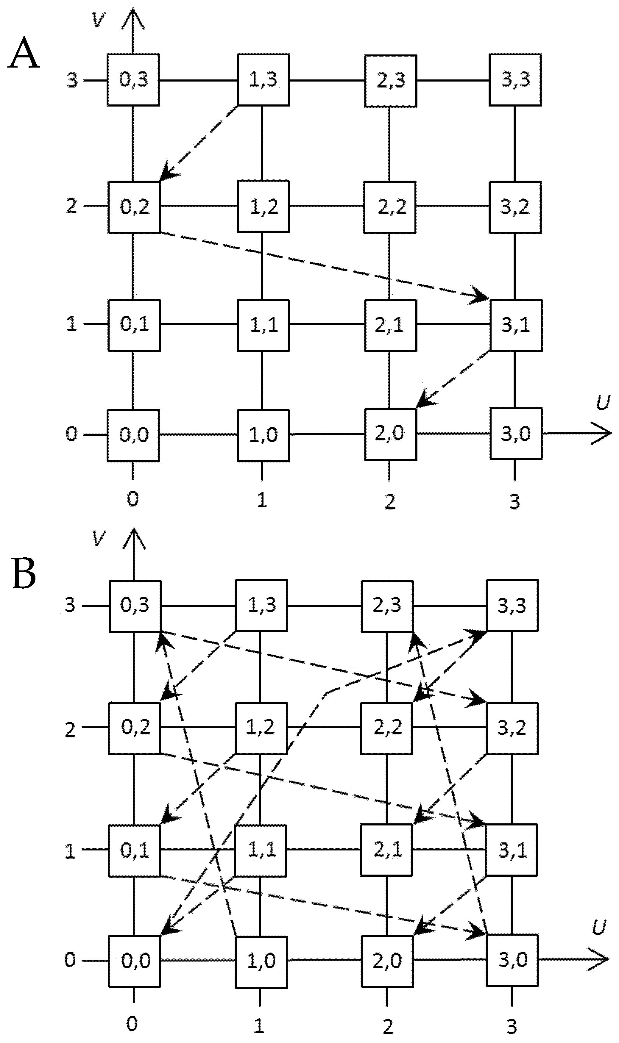
Next, the Descartes plane could be labeled as stochastic if a topological (meaning logically connected) transition from one point to another can be performed randomly. In [49] the generator nsDeonYuliPlaneTwist32D was introduced to create all the stochastic uniform sequences without skipping or repeating the elements. All cells of the grid are taken into account, and the aforementioned property is fully satisfied. Figure 7 shows how the possible transitions between points along a stochastic path are performed. It should be noted that Figure 7 demonstrates only one of the possible ways to implement the transition process, although in reality they may reach over several thousand.
As an example, in the program code DMP0103, it is shown how to organize and create such a generation for a square photomatrix with a size of cells. Such a small range is selected only for visual presentation in this article, but for the real task the range of construction could be chosen for any size.
        using nsDeonYuliPlaneTwist32D;    //plane twist generator
        namespace DMP0103
        { class cDMP0103
         { static void Main(string[[] args)
          { cDeonYuliPlaneTwist32D TP =
                 new cDeonYuliPlaneTwist32D();
           int w = 3;      // random number bit length
           int N = 1 << w;        // track length
           TP.SetW(w);
           TP.Start();         // generator start
           Console.WriteLine("w = {0}  N = {1}", w, N);
           int[[,] A = new int[N, N];     // result matrix
           for (int i = 0; i < N; i++)
            for (int j = 0; j < N; j++) A[i, j] = 0;
           uint u = 0;    // point job coordinates on plane
           uint v = 0;
           for (int i = 0; i < N; i++)
            for (int j = 0; j < N; j++)
            { TP.Next(ref u, ref v);    // point on grid
              A[u, v]++;   // generation counter for <u,v>
            }
           Console.WriteLine("Matrix A");
           for (int i = 0; i < N; i++)
           {  for (int j = 0; j < N; j++)
             Console.Write("{0,4}", A[i, j]);
            Console.WriteLine();
           }
           Console.ReadKey();       // result viewing
          }
         }
        }
After starting this program, the result of generation appears in the following form.
        w = 3 N = 8
        Matrix A
        1 1 1 1 1 1 1 1
        1 1 1 1 1 1 1 1
        1 1 1 1 1 1 1 1
        1 1 1 1 1 1 1 1
        1 1 1 1 1 1 1 1
        1 1 1 1 1 1 1 1
        1 1 1 1 1 1 1 1
        1 1 1 1 1 1 1 1
This printout confirms that in matrix A each point source of cell grid (or LED, in the context of PMTS construction) is randomly turned on exactly once, ensuring the property of uniformity over the entire plane. It is necessary to obtain exactly this result for software applications that target the stochastic design of PMTS. In our case we have just achieved it.
4. Discussion
The above proposed and analyzed algorithm for the stochastic switching on the LED sources uses twisting sequences U and V. The generation begins with a congruent sequence in which the next random variable is calculated from the value of the previous random variable as follows:
The mathematical operation modulus forms the remainder of integer division of . This allows for keeping the values of random variables and in the interval . There is no skipping of numbers in uniform sequences, and none of them are repeated. Thus, the uniform sequence of numbers from the interval contains exactly N numbers. Therefore, operation in Expression (1) coincides with the length N of the stochastic sequence.
In Expression (26) the form of the function can be taken arbitrarily. The most common option for this realization is a linear function in the following form:
Substituting (27) into (26), it is possible to obtain a congruent linear dependence of the sequential generation of random variables:
Formally, congruent generation (28) could not be considered as an absolutely complete probabilistic space [46], since in the field of congruent sequences, using Gödel’s theorem on the arithmetic incompleteness of factorial transformations, it is impossible to completely create all the stochastic sequences. In such cases, pseudorandom variables are usually referred to. However, in practical implementation, for example in our case of the stochastic PMTS designing, an absolutely complete probabilistic space, which is inherent in theoretical problems, is not required. Specifically, in our case, this follows from the fact that irradiation interval by LED source has a limited time period , which in turn provides a total finite time of full exposure in form as ).
Thus, the physical time restrictions on the switching on and off the LEDs, taking into account the effectiveness of the impact on the biological tissue of the human body, do not allow theoretical stochastic implementation over complete probabilistic space. In other words, PMTS in reality is able to perform only a limited probabilistic realization of the stochastic process. This is sufficient for practical implementation to reliably describe a probabilistic (or partial in the number of probabilistic options, i.e., pseudo-probabilistic) random plane.
Moving further, it could be be noted that Expression (28) also has some limitations. The first of which concerns the number N. Our mathematical studies [46,47,48,49,50,51] show that uniform generation is achieved only at the condition of . The exponent w exactly matches the quantity of the required binary bits, which are needed for representing the decimal number . These w bits contain gradations of representations of all numbers from the interval .
The second restriction relates to the multiplicative constant a in Expression (28). First of all, constant a must not be outside the range of random variables . The uniform sequences consisting of N random variables are possible only when the following condition is satisfied:
The third issue concerns the additive constant c in Expression (28). There is the same requirement for constant c, i.e., it must not be outside the range of random variables . In addition, only odd values are allowed for this constant:
Now it is time to provide some calculations. For example, Expressions (29) and (30) together give the following amount of congruent pairs to generate the same number of congruent sequences:
Thus, Expression (31) shows the total quantity of possible congruent sequences having a length of random variables.
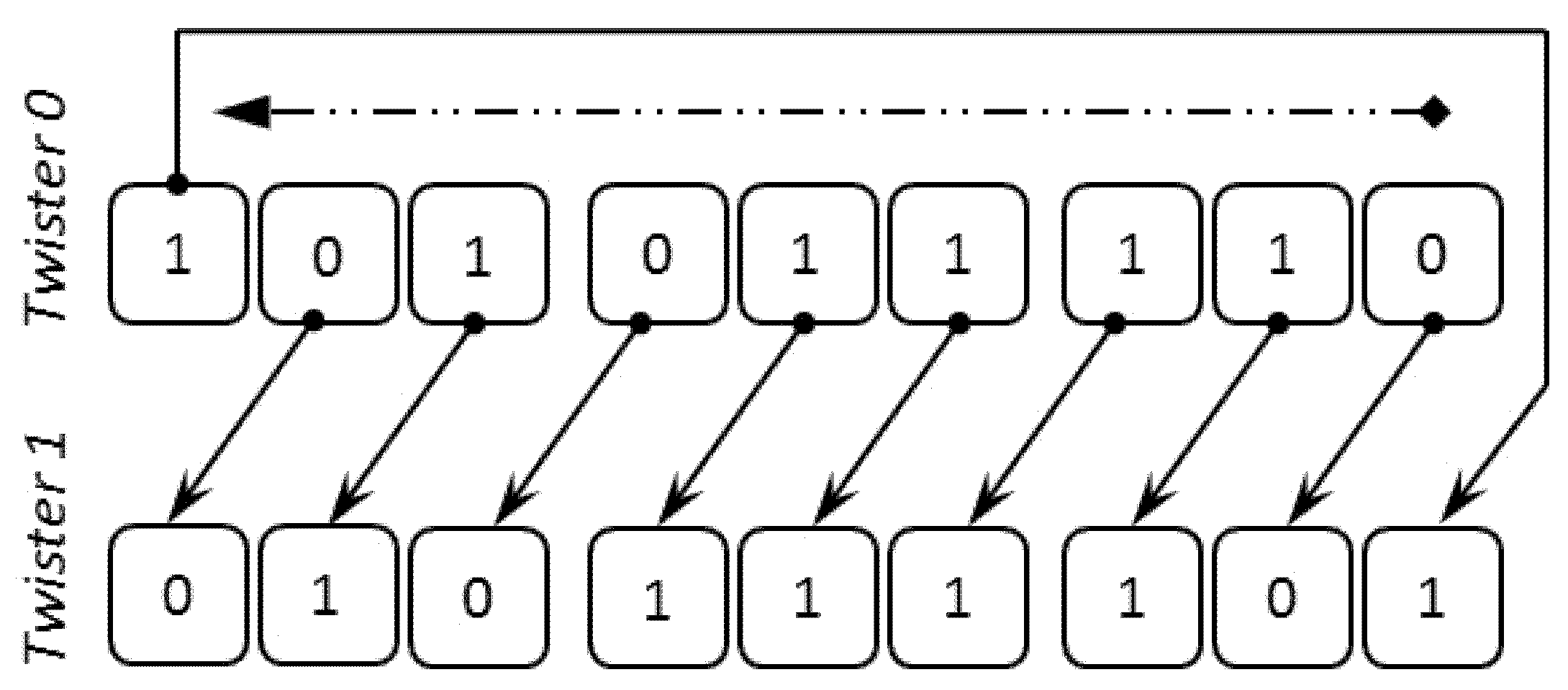
In stochastic PMTS the uniform twister plane generator nsDeonYuliPlaneTwist32D is used. In its twisting generations, the initial congruent sequence is Twister 0, which has a binary representation. The subsequent Twister 1 is organized according to the circular algorithm by simultaneously shifting all the numbers of the initial congruent sequence by one bit. As an example, Figure 8 shows a one-bit shift to the left for a sequence of three numbers . The result of this shift is that the new sequence is obtained.
Therefore, the acquired twisting sequences are complete and contain the uniform random variables without skipping or repetitions. Moreover, twisting sequences are not linearly congruent. The amount , which characterizes the total number of congruent and twisting sequences together, is determined as follows:
The amount of a complete set of random planes for one pair of congruent coefficients a and c is obtained by multiplying and w; this characterizes the number of different twisters including the congruent Twister 0:
Furthermore, taking into account all the pairs of congruent coefficients a and c, the total number of generated twisting stochastic planes for one PMTS is determined by the following expression:
Thus, Expression (9) shows the total number of different actions of uniformly switching on the LEDs located on the PMTS plane surface.
The problem of finding a solution for generating the uniform discrete twisting planes having the Descartes properties of the single presence of random points in a discrete matrix has been completed. In the context of this article it means that the task of creating software tools for providing the uniform stochastic twister generation of LED irradiation by PMTS is solved.
5. Conclusions
Analysis of the source material shows that the algorithms used by ordinary random number generators for plane realization do not take into account the advantages of absolutely uniform sequences of random variables. The generation technologies used in them do not guarantee the absolute uniformity of the completely random planes. Direct use of twisting generators of uniform sequences, for example nsDeonYuliTwist32D, is limited by the properties of Descartes uniform planes regarding the location of points. Using a technology of secondary indexing allows for creating the twister plane generator nsDeonYuliPlaneTwist32D, which ensures the completeness and uniqueness of all the random variables on the grid of the Descartes plane. In addition, using a variety of initial twisting sequences makes it possible to obtain new functional capabilities for PMTS. Specifically in our case, we demonstrated this possibility for constructing the uniform stochastic PMTS using LED irradiation sources.
Author Contributions
Conceptualization, Paper writing—original draft preparation, investigation, programming, validation, data curation, visualization, formal analysis, O.K.K.; Paper writing—original draft preparation and editing, conceptualization and methodology, software, programming and analysis, algorithm improvement, data curation, resources, A.F.D.; Paper writing—original draft preparation, review and editing, conceptualization and methodology, validation, project administration and supervision, resources and funding acquisition, Y.A.M. All authors have read and agreed to the published version of the manuscript.
Funding
This work was supported by Burroughs Wellcome Fund 2019, Award ID: AWD00053567.
Acknowledgments
The authors are thankful to Matthew Vandenberg, J. Alex Watts, Jacqueline Nolan, Mohsen Sharifi and Robert Weingold for the proofreading.
Conflicts of Interest
The authors declare that there are no conflicts of interest regarding the publication of this article.
References
- Menyaev, Y.A.; Zharov, V.P. Experience in development of therapeutic photomatrix equipment. Biomed. Eng. 2006, 40, 57–63. [Google Scholar] [CrossRef]
- Menyaev, Y.A.; Zharov, V.P. Experience in the use of therapeutic photomatrix equipment. Biomed. Eng. 2006, 40, 144–147. [Google Scholar] [CrossRef]
- Menyaev, Y.A.; Zharov, V.P. Phototherapeutic technologies for oncology. Proc. SPIE 2005, 5973, 271–278. [Google Scholar] [CrossRef]
- Zharov, V.P.; Zmievskoi, G.N.; Meniaev, I.; Salishchev, D.N.; Kalinin, K.I.; Stepanchuk, N. Development of an algorithm for calculating the spatial distribution of the radiation intensity of photomatrix therapeutic apparatuses. Biomed. Eng. 2002, 36, 188–194. [Google Scholar] [CrossRef]
- Zharov, V.P.; Menyaev, Y.A.; Gorchak, Y.Y.; Utkina, K.V.; Menyaev, Y.A. Methods for photoultrasonic treatment of festering wounds in oncological patients. Crit. Rev. Biomed. Eng. 2001, 29, 111–124. [Google Scholar] [CrossRef] [PubMed]
- Zharov, V.P.; Menyaev, Y.A.; Kabisov, R.K.; Al’kov, S.V.; Nesterov, A.V.; Savrasov, G.V. Design and application of low-frequency ultrasound and its combination with laser radiation in surgery and therapy. Crit. Rev. Biomed. Eng. 2001, 29, 502–519. [Google Scholar] [CrossRef]
- Menyaev, Y.A.; Zharova, I.Z. A technique for surgical treatment of infected wounds based on photodynamic and ultrasound therapy. Biomed. Eng. 2006, 40, 284–290. [Google Scholar] [CrossRef]
- Menyaev, Y.A.; Zharov, V.P.; Mishanin, E.A.; Kuzmich, A.P.; Bessonov, S.E. Combined photovacuum therapy of copulative dysfunction. Proc. SPIE 2006, 6078, 241–248. [Google Scholar] [CrossRef]
- Menyaev, Y.A.; Zharov, V.P. Combination of photodynamic and ultrasonic therapy for treatment of infected wounds in animal model. Proc. SPIE 2006, 6087, 30–39. [Google Scholar] [CrossRef]
- Vel’sher, L.Z.; Podkolzin, A.A.; Stakhanov, M.L.; Gorchak, Y.Y.; Zharov, V.P.; Menyaev, Y.A.; Zmievskoi, G.N.; Rozhdestvin, V.N. A combined method for wound treatment based on exposure to low-intensity radiation and ultrasound. Biomed. Eng. 2003, 37, 262–267. [Google Scholar] [CrossRef]
- Zharov, V.P.; Kalinin, K.I.; Menyaev, Y.A.; Zmievskoy, G.N.; Savin, A.A.; Stulin, I.D.; Shihkerimov, R.K.; Shapkina, A.V.; Velsher, L.Z.; Stakhanov, M.L. Phototherapeutic treatment of patients with peripheral nervous system diseases by means of LED arrays. Proc. SPIE 2001, 4244, 143–151. [Google Scholar] [CrossRef]
- Zharov, V.P.; Menyaev, Y.A.; Kalinin, K.L.; Zmievskoy, G.N.; Velsher, L.Z.; Podkolzin, A.A.; Stakhanov, M.L.; Gorchak, Y.Y.; Sarantsev, V.P. Combined photoultrasonic treatment of infected wounds. Proc. SPIE 2001, 4244, 133–142. [Google Scholar] [CrossRef]
- Zharov, V.P.; Menyaev, Y.A.; Gorchak, Y.V.; Zmievskoi, G.N.; Bagdasarov, V.V.; Ambrozevich, E.G.; Shchepilov, D.V.; Kazarova, E.A. Photoultrasonic treatment of septic wounds. Biomed. Eng. 2001, 35, 6–10. [Google Scholar] [CrossRef]
- Gu, Y.; Qiu, H.; Wang, Y.; Huang, N.; Liu, T.C.Y. Light-Emitting Diodes for Healthcare and Well-being: Materials, Processes, Devices and Applications. In Light-Emitting Diodes; Springer: Berlin/Heidelberg, Germany, 2019; pp. 485–511. [Google Scholar] [CrossRef]
- Hadis, M.A.; Cooper, P.R.; Milward, M.R.; Gorecki, P.C.; Tarte, E.; Churm, J.; Palin, W.M. Development and application of LED arrays for use in phototherapy research. J. Biophotonics 2017, 10, 1514–1525. [Google Scholar] [CrossRef]
- Zhang, Y.; Wang, J.; Guo, L.; Xiong, D. Design of a multi-band LED phototherapy system with therapeutic evaluation. Proc. SPIE 2019, 11334. [Google Scholar] [CrossRef]
- Akşahin, M. Multifunctional phototherapy device design. Electrica 2019, 19, 65–71. [Google Scholar] [CrossRef] [Green Version]
- Kohli, H.; Srivastava, S.; Sharma, S.K.; Chouhan, S.; Oza, M. Design of Programmable LED Based Phototherapy System. Int. J. Opt. 2019, 1–8. [Google Scholar] [CrossRef]
- Ugarte, M.F.; Chávarri, L.; Briz, S. Note: Design of a dose-controlled phototherapy system based on hyperspectral studies. Rev. Sci. Instrum. 2013, 84. [Google Scholar] [CrossRef]
- Ugarte, M.F.; Chávarri, L.; Briz, S.; Padrón, V.M.; García-Cuesta, E. Active multispectral imaging system for photodiagnosis and personalized phototherapies. Rev. Sci. Instrum. 2014, 85. [Google Scholar] [CrossRef]
- Sorbellini, E.; Rucco, M.; Rinaldi, F. Photodynamic and photobiological effects of light-emitting diode (LED) therapy in dermatological disease: An update. Lasers Med. Sci. 2018, 33, 1431–1439. [Google Scholar] [CrossRef] [Green Version]
- Sauder, D.N. Light-emitting diodes: Their role in skin rejuvenation. Int. J. Dermatol. 2010, 49, 12–16. [Google Scholar] [CrossRef]
- Gutta, S.; Shenoy, J.; Kamath, S.P.; Mithra, M.; Baliga, S.; Sarpangala, M.; Mukund, P.S. Light Emitting Diode (LED) Phototherapy versus Conventional Phototherapy in Neonatal Hyperbilirubinemia: A Single Blinded Randomized Control Trial from Coastal India. BioMed. Res. Int. 2019, 2019, 1–6. [Google Scholar] [CrossRef] [Green Version]
- Foley, J.S.; David, B.; Bradle, V.J.; Rudio, C.; Calderhead, R.G. 830 nm light-emitting diode (led) phototherapy significantly reduced return-to-play in injured university athletes: A pilot study. Laser Ther. 2016, 25, 35–42. [Google Scholar] [CrossRef] [Green Version]
- Karaduta, O.; Zaman, L. Shk-9: A new tool in approach of glycoprotein annotation. Software 2018, 7, 302–303. [Google Scholar] [CrossRef]
- Menyaev, Y.A.; Nedosekin, D.A.; Sarimollaoglu, M.; Juratli, M.A.; Galanzha, E.I.; Tuchin, V.V.; Zharov, V.P. Optical Clearing in Photoacoustic Flow Cytometry. Biomed. Opt. Express 2013, 4, 3030–3041. [Google Scholar] [CrossRef] [Green Version]
- Menyaev, Y.A.; Carey, K.A.; Nedosekin, D.A.; Sarimollaoglu, M.; Galanzha, E.I.; Stumhofer, J.S.; Zharov, V.P. Preclinical Photoacoustic Models: Application for Ultrasensitive Single Cell Malaria Diagnosis in Large Vein and Artery. Biomed. Opt. Express 2016, 7, 3643–3658. [Google Scholar] [CrossRef] [Green Version]
- Moreno, I. Image-like illumination with LED arrays: Design. Opt. Lett. 2012, 37, 839–841. [Google Scholar] [CrossRef]
- Wang, K.; Wu, D.; Qin, Z.; Chen, F.; Luo, X.; Liu, S. New reversing design method for LED uniform illumination. Opt. Express 2011, 19, A830–A840. [Google Scholar] [CrossRef]
- Su, Z.; Xue, D.; Ji, Z. Designing LED array for uniform illumination distribution by simulated annealing algorithm. Opt. Express 2012, 20, A843–A855. [Google Scholar] [CrossRef]
- Abeysekera, S.K.; Kalavally, V.; Ooi, M.; Kuang, Y.C. Impact of circadian tuning on the illuminance and color uniformity of a multichannel luminaire with spatially optimized LED placement. Opt. Express 2020, 28, 130–145. [Google Scholar] [CrossRef]
- Wu, R.; Zheng, Z.; Li, H.; Liu, X. Optimization design of irradiance array for LED uniform rectangular illumination. Appl. Opt. 2012, 51, 2257–2263. [Google Scholar] [CrossRef]
- Pal, S. Optimization of LED array for uniform illumination over a target plane by evolutionary programming. Appl. Opt. 2015, 54, 8221–8227. [Google Scholar] [CrossRef]
- Liu, P.; Wang, H.; Wu, R.; Yang, Y.; Zhang, Y.; Zheng, Z.; Li, H.; Liu, X. Uniform illumination design by configuration of LEDs and optimization of LED lens for large-scale color-mixing applications. Appl. Opt. 2013, 52, 3998–4005. [Google Scholar] [CrossRef]
- Li, S.; Wang, K.; Chen, F.; Liu, S. New freeform lenses for white LEDs with high color spatial uniformity. Opt. Express 2012, 20, 24418–24428. [Google Scholar] [CrossRef]
- Teng, T.C.; Sun, W.S.; Lin, J.L. Designing an LED luminaire with balance between uniformity of luminance and illuminance for non-Lambertian road surfaces. Appl. Opt. 2017, 56, 2604–2613. [Google Scholar] [CrossRef]
- Zhao, Z.; Zhang, H.; Liu, S.; Wang, X. Effective freeform TIR lens designed for LEDs with high angular color uniformity. Appl. Opt. 2018, 57, 4216–4221. [Google Scholar] [CrossRef]
- Feller, W. An Introduction to Probability Theory and Its Applications, 3rd ed.; John Wiley & Sons: Hoboken, NJ, USA, 2008; p. 528. [Google Scholar]
- Gnedenko, B. Theory of Probability, 6th ed.; CRC Press: Boca Raton, FL, USA, 1998; p. 520. [Google Scholar]
- Kolmogorov, A.N.; Fomin, S.V. Elements of the Theory of Functions and Functional Analysis, 1st ed.; Dover Publications: Mineola, NY, USA, 1999; p. 128. [Google Scholar]
- Cramer, H. Mathematical Methods of Statistics, 1st ed.; Princeton University Press: Princeton, NJ, USA, 1999; p. 575. [Google Scholar]
- Knuth, D.E. Art of Computer Programming, Volume 2: Seminumerical Algorithms, 3rd ed.; Addison-Wesle: Boston, MA, USA, 2014; p. 784. [Google Scholar]
- Knuth, D.E. Art of Computer Programming, Volume 4A: Combinatorial Algorithms, Part 1, 1st ed.; Addison-Wesley: Boston, MA, USA, 2011; p. 912. [Google Scholar]
- van der Waerden, B.L. Algebra: Volume, I; Springer: New York, NY, USA, 1991; p. 265. ISBN 978-0-387-40624-4. [Google Scholar]
- van der Waerden, B.L. Algebra: Volume II; Springer: New York, NY, USA, 1991; p. 284. ISBN 978-0-387-40625-1. [Google Scholar]
- Deon, A.F.; Menyaev, Y.A. The Complete Set Simulation of Stochastic Sequences without Repeated and Skipped Elements. J. Univers. Comput. Sci. 2016, 22, 1023–1047. [Google Scholar] [CrossRef]
- Deon, A.F.; Menyaev, Y.A. Parametrical Tuning of Twisting Generators. J. Comput. Sci. 2016, 12, 363–378. [Google Scholar] [CrossRef] [Green Version]
- Deon, A.F.; Menyaev, Y.A. Twister Generator of Arbitrary Uniform Sequences. J. Univers. Comput. Sci. 2017, 23, 353–384. [Google Scholar] [CrossRef]
- Deon, A.F.; Menyaev, Y.A. The Uniform Twister Plane Generator. J. Comput. Sci. 2018, 14, 260–272. [Google Scholar] [CrossRef] [Green Version]
- Deon, A.; Menyaev, Y. Poisson Twister Generator by Cumulative Frequency Technology. Algorithms 2019, 114, 114. [Google Scholar] [CrossRef] [Green Version]
- Deon, A.F.; Menyaev, Y.A. Twister Generator of Random Normal Numbers by Box-Muller Model. J. Comput. Sci. 2020, 16, 1–13. [Google Scholar] [CrossRef] [Green Version]
- Matsumoto, M.; Nishimura, T. Mersenne twister: A 623-dimensionnally Equidistributed Uniform Pseudorandom Number Generator. ACM Trans. Modeling Comput. Simul. 1998, 8, 3–30. [Google Scholar] [CrossRef] [Green Version]
- Sutton, C.; McCallum, A. An Introduction to Conditional Random Fields. Found. Trends Mach. Learn. 2012, 4, 267–373. [Google Scholar] [CrossRef]
- Quattoni, A.; Collins, M.; Darrell, T. Conditional Random Fields for Object Recognition. In Proceedings of the 17th International Conference on Neural Information Processing Systems, Denver, CO, USA, 3–10 December 2004; pp. 1097–1104. [Google Scholar]
- Bekkerman, R.; Sahami, M.; Learned-Miller, E. Combinatorial Markov Random Fields. In Proceedings of the 17th European Conference on Machine Learning, Berlin, Germany, 18 September 2006; pp. 30–41. [Google Scholar] [CrossRef] [Green Version]
- Sarawagi, S.; Cohen, W.W. Semi-Markov Conditional Random Fields for Information Extraction. In Proceedings of the 17th International Conference on Neural Information Processing Systems, Barcelona, Spain, 4–11 December 2005; pp. 1185–1192. [Google Scholar]
- Rimstad, K.; Omre, H. Skew-Gaussian Random Fields. Spat. Stat. 2014, 10, 43–62. [Google Scholar] [CrossRef] [Green Version]
- Xiao, Y. Uniform Modulus of Continuity of Random Fields. Monatshefte für Mathematik 2010, 159, 163–184. [Google Scholar] [CrossRef] [Green Version]
- Qi, Y.; Szummer, M.; Minka, T.P. Bayesian Conditional Random Fields. In Proceedings of the AISTATS’05: 10th International Workshop on Artificial Intelligence and Statistics, Savannah, Barbados, 6–8 January 2005; pp. 269–276. [Google Scholar]
Figure 1.
Varieties of photomatrix therapeutic systems (description of pictures is provided in text).
Figure 1.
Varieties of photomatrix therapeutic systems (description of pictures is provided in text).

Figure 2.
Initial schematics for calculation of illuminance of a single LED point source.

Figure 3.
Simple schematics for calculation of illuminance produced by flat PMTS.

Figure 4.
Three general types of PMTS (flat, cylindrical and spherical) and position of basic coordinate system for calculation of PMTS illuminance.
Figure 4.
Three general types of PMTS (flat, cylindrical and spherical) and position of basic coordinate system for calculation of PMTS illuminance.

Figure 5.
Schematics with main parameters for calculation of cylindrical PMTS.

Figure 6.
Schematics with main parameters for calculation of spherical PMTS.

Figure 7.
(A) A random track and (B) a possible set of tracks for one complete stochastic matrix.

Figure 8.
Diagram of circular twister algorithm.

© 2020 by the authors. Licensee MDPI, Basel, Switzerland. This article is an open access article distributed under the terms and conditions of the Creative Commons Attribution (CC BY) license (http://creativecommons.org/licenses/by/4.0/).
Share and Cite
MDPI and ACS Style
Karaduta, O.K.; Deon, A.F.; Menyaev, Y.A. Designing the Uniform Stochastic Photomatrix Therapeutic Systems. Algorithms 2020, 13, 41. https://0-doi-org.brum.beds.ac.uk/10.3390/a13020041
AMA Style
Karaduta OK, Deon AF, Menyaev YA. Designing the Uniform Stochastic Photomatrix Therapeutic Systems. Algorithms. 2020; 13(2):41. https://0-doi-org.brum.beds.ac.uk/10.3390/a13020041
Chicago/Turabian StyleKaraduta, Oleg K., Aleksei F. Deon, and Yulian A. Menyaev. 2020. "Designing the Uniform Stochastic Photomatrix Therapeutic Systems" Algorithms 13, no. 2: 41. https://0-doi-org.brum.beds.ac.uk/10.3390/a13020041
Note that from the first issue of 2016, this journal uses article numbers instead of page numbers. See further details here.