Model of Multi-branch Trees for Efficient Resource Allocation


1
Faculty of Teacher Education, Shumei University, Chiba 276-0003, Japan
2
Faculty of Tourism and Business Management, Shumei University, Chiba 276-0003, Japan
3
Faculty of Business Administration, Soka University, Tokyo 192-8577, Japan
4
Department of Information Systems and Operations, Vienna University of Economics, 1020 Wien, Austria
*
Author to whom correspondence should be addressed.
Algorithms 2020, 13(3), 55; https://0-doi-org.brum.beds.ac.uk/10.3390/a13030055
Submission received: 12 February 2020
/
Revised: 27 February 2020
/
Accepted: 28 February 2020
/
Published: 1 March 2020
Abstract
:Although exploring the principles of resource allocation is still important in many fields, little is known about appropriate methods for optimal resource allocation thus far. This is because we should consider many issues including opposing interests between many types of stakeholders. Here, we develop a new allocation method to resolve budget conflicts. To do so, we consider two points—minimizing assessment costs and satisfying allocational efficiency. In our method, an evaluator’s assessment is restricted to one’s own projects in one’s own department, and both an executive’s and mid-level executives’ assessments are also restricted to each representative project in each branch or department they manage. At the same time, we develop a calculation method to integrate such assessments by using a multi-branch tree structure, where a set of leaf nodes represents projects and a set of non-leaf nodes represents either directors or executives. Our method is incentive-compatible because no director has any incentive to make fallacious assessments.
1. Introduction
Exploring the principles of resource allocation is still important in many fields. Although, in many disciplines, including finance [1,2,3], economics [4,5,6], politics [7,8], marketing [9], and engineering [10,11,12], many approaches such as Pareto efficiency [13] or Inequality Reexamined [14] have been proposed for efficient resource allocation, little is known about appropriate methods for optimal resource allocation thus far. This is because such methods should solve lots of issues. For instance, the number of stakeholders who are operating from different standpoints is not small. Hence, the meaning of “optimal” differs between each stakeholder, so it is difficult for them to reach a good consensus. Not only that, there exist some practical restrictions such as limited resources or insufficient amounts of time. Therefore, developing appropriate budget allocation methods is still an issue. In addition, examining performance measurements for budgetary decision-making is also important for developing effective budget allocation methods [15].
Cooperative game literature has many studies on efficient resource allocation [16,17]. In particular, the core and kernel in cooperative game theory propose concrete feasible allocation. However, this method requires not only assessment values measuring all objects for allocation but also those values of any coalition of objects. Such a characteristic of requiring perfect information is almost impossible to satisfy in many real situations because all objects must be assessed with a unique measurement policy to do so.
The field of resource allocation has few unique measurement policies for assessing an object, although GMAT (Graduate Management Admission Test), for example, provides a unique measurement for measuring some skills of pupils for business school [18]. Let us consider a competitive fund organized by a national institution. Thousands of research agendas are submitted in Japan [19]. If the total required budget exceeds the available budget, the agendas should be selected. In this situation, no one knows a unified criterion for measuring all agendas, and thus, agendas are actually categorized into many small disciplines, which introduces too much segmentation. In each discipline, a feasible number of agendas are considered and selected. The important issue with this method is how much budget is distributed to each discipline. Normally, a primitive method is adopted. In Japanese competitive funds, a budget is divided and distributed to each discipline in proportion to the number of submitted agendas. That is, the acceptance rates of any of the disciplines are controlled the same or almost the same as each other.
Local governments are facing the same issue. In Japan, two kinds of budget allocation systems are generally used. One is a system in which budget allocators examine all projects. The system can force allocators to use their extensive powers and resources, though it can lead to quite appropriate allocations. The other is a system in which a budget allocator provides budget ceilings to each section for each policy. This is based on precedent or incrementalism. Although the first system has been in use for a long time, budget allocators are likely to avoid the system due to the huge costs needed. This is why a Japanese nationwide scale questionnaire survey [20] found that some local governments have switched to the second system. However, there is still a room for further improvement with this second system [21]. In fact, we find that a certain city abolished the second system after adopting it for ten fiscal years [22].
Although local governments in Japan consider such incrementalism for solving budget battles, such a simple but rigid rule cannot capture actual needs, and thus, it is difficult to respond to environmental changes adaptively. Not only that, it may lead to sectarianism, where winning budget battles and getting money for one’s department are an absolute must. Moreover, they tend to spend budgets wastefully at the end of a fiscal year.
With this research background in mind, the objective of our study is to find a feasible allocation method that is better than the primitive method based on incrementalism [23,24] even if there is no appropriate unified criterion. Here, we propose an allocation method that can distribute budgets efficiently with imperfect information, not perfect information, in cooperative games.
To do so, we consider two points: minimizing assessment costs and satisfying allocational efficiency. Assessment costs here mean the costs of effort spent on assessments including the costs of designing a unified criterion that can be applied to all objects for allocation. Actually, designing such a criterion is almost impossible, and thus, we should consider a method that determines all allocation by integrating many assessments, the scope of which is local only. We developed a method in which multiple evaluators assess all objects for allocation in a manner like the division of labor, and allocation is calculated by integrating those assessments. Our method minimizes assessment costs.
The second point, allocational efficiency, is also an important issue. Let us consider a department where two projects would like to get money. The director of the department may be one the best people to assign money to those projects. Therefore, the director’s assessment on the relative weights between the two can be extremely important information when considering budget allocation. We believe that the popularity of the allocation method based on incrementalism and precedent that is widely adopted in Japan is empirical evidence that budgets being distributed by directors to their own projects in their department is one of the most effective allocation methods.
Thus, are there any allocation methods that are more rational than a method that uses budget ceilings based on incrementalism? To consider this point, let us consider a small company that is working on budget allocation. The executive is the person in charge of the allocation, and there are several departments in the company. Each department is managed by a director and has several projects to which part of the budget needs to be assigned. If the directors precisely assess the rates of allocation for the projects in their departments, is it possible to regard assessing one project only among all projects as an assessment of all projects in the departments? An executive cannot consider all projects in one’s company; however, if the executive selects one project in each department, it can be considered that the executive assesses all projects due to supporting by the directors who assess the remaining projects. The executive may not understand each project in detail. In this case, however, the executive can request that the directors send reports on the selected projects. By doing this, the executive may know the selected projects as do the directors. The executive can assess the relative values between departments from their own viewpoint by comparing each selected project.
Here, we propose a protocol of allocation based on the above discussion. In this protocol, a director’s assessment is restricted to one’s own projects in one’s own department, and both an executive’s and mid-level executives’ assessments are also restricted to each representative project in each of the branches or departments that they manage. At the same time, we develop a calculation method to integrate such assessments. In our method, we use a multi-branch tree structure, where a set of leaf nodes represents either projects or policies and a set of non-leaf nodes represents either directors or executives. Our method may be balanced between minimizing assessment costs and allocational efficiency, and thus, we believe it to be novel.
The rest of this paper is organized as follows. We describe our novel budget allocation method for both a tournament model and a generalized model in Section 2. Some examples are provided in Section 3. We analyze some salient features in Section 4. We then discuss the features of our method and a further study in Section 5.
2. Methods
We define the new budget allocation method as a multi-branch tree structure. First, we define some terms, variables, and maps in the first subsection. Next, we explain the procedure of our method. In the procedure, we calculate a final allocation. This calculation of a specific type is easier than the generalized type; thus, we first introduce the specific type, called the “tournament model” and finally, we introduce the generalized model.
2.1. Notation
Let us consider that an organization is considering distributing its budget to projects where the number of projects is set to N. Each project belongs to a department. A department has at least one project. A manager of a department is called a director. The top of the organization is called an executive. The executive manages all departments either directly or indirectly. If the executive manages them indirectly, there are mid-level departments managed by mid-level executives managing either departments or mid-level departments. This organizational structure is drawn as a tree structure using graph theory.
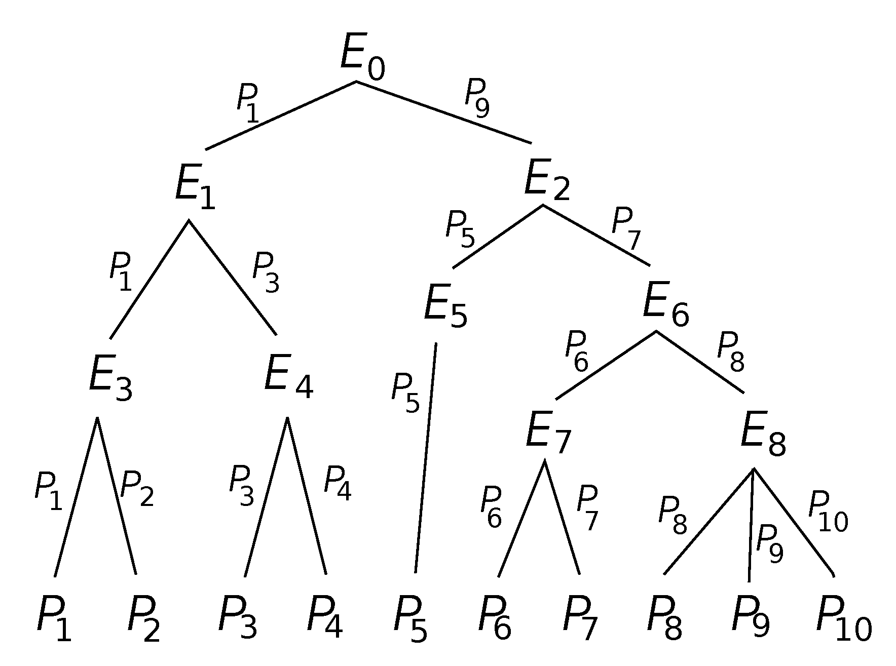
Figure 1 shows an example of an organization. There are 10 projects () that require money, 5 departments (whose directors are , and ), and 3 mid-level executives (, and ) and 1 executive () in the organization. The departments own projects are for , for , for , for , and for .
We define a multi-branch tree structure , where n is the number of leaf nodes representing projects, and m is that of internal nodes representing evaluators consisting of directors, mid-executives, and an executive. P denotes a set of leaf nodes , and E denotes a set of non-leaf nodes . We call the root node (the executive) and the others internal nodes. The example tree of Figure 1 is defined as with 10 projects and 9 evaluators.
For any , we denote by a tree consisting of and all of its descendent nodes. Note that . Let be the set of all child nodes of and the set of the index numbers of evaluators in . A tree is called a child tree of . Here, we call the set of child trees of . For example, is obtained from in the example tree of Figure 1.
Next, we define a map as
where h means the length of the path from to . In contrast, we define a map as
which outputs an index number of , where h means the length of the path from to . Note that if is not a descendant leaf node of , we have , and is not defined.
For any , we obtain only one shortest path from to and call it path i. For example, we consider in Figure 1. The parent node of is , and the parent node of is . Repeating this procedure, we finally reach the root node, . We then solve path 7 as follows.
Note that every path i for is a sequence from to .
2.2. Procedure
We explain the procedure of our method. First, we define all projects as objects for distributing a budget, departments, directors, and executives as defined above. The second paragraph of the Notation Subsection shows these terms with the example of Figure 1.
Step 1 Selection
First, all evaluators select projects that they must assess. However, all evaluators are prohibited from assessing them before all assessments are done by those who are children. In the example of Figure 1, must wait until assessment by and is finished, and must wait until all assessments by to are finished.
A set of projects assessed by any evaluator is determined with the following procedure. If an evaluator is a director (who directly connects with leaf nodes), the director selects all projects in one’s own department. In the example of Figure 1, a set of projects for is , and a set of projects for is . If an evaluator is not a director (that is, either an executive or a mid-level executive), one selects a project among descendant leaves of one’s child node each. In the example of Figure 1, must select two projects; one is from descendant leaves of , and the other is from descendant leaves of . In this case, all combinations are , , , and . Among them, selects a set. In the example of Figure 1, a set of projects for is . Note that the label of every branch in Figure 1 is a selected project.
Step 2 Evaluation
Second, all evaluators assess the projects that they must assess. They give a positive real number to each project as an assessment value. For capturing these values, we define a map , where means the evaluation value that gives .
Note that an assessment is given relatively. Let us consider that evaluator assesses two projects, and , as shown in Figure 1. The assessment values of the two are denoted as and , respectively. However, these values are relative to each other. That is, the case of giving and is completely equivalent to the case of giving and .
Step 3 Calculation
In the final step, the final allocation of budgets is calculated. To do so, we first calculate an N-dimensional vector
which consists of rates of allocation. Therefore, . Using this vector, the executive distributes to , where G is the gross of the budget.
Each element of W must correspond to each evaluator’s assessment. That is, for any evaluator and for any two projects and where assesses both and , . We developed a calculation method to solve W in the following subsections.
2.3. Tournament Model
First, we consider a specific case, called the “tournament model”. In this model, any evaluator except for the directors must satisfy a tournament condition where an evaluator selects projects that were selected by the evaluator’s child evaluators. In the example of Figure 1, a set of projects for is and , and both being selected by and being selected by is satisfied. Therefore, satisfies the tournament condition. In comparison, the set of projects for is and , but is not selected by . Therefore, does not satisfy the tournament condition. There is an evaluator who does not satisfy the tournament condition in Figure 1, and thus, Figure 1 is not a tournament model.
In the tournament model, all evaluators have restricted candidate sets for selecting projects. However, the relative weight vector, W, is easily calculated. To explain this point, we define some notations. Let be the set of projects from which chooses projects for each . Note that is the only one evaluator included both in and path i for in path i. It is easy to see that should choose a project from . Define a map that outputs an index number of , where is chosen by as a selected project of . We label the edge that connects to “” as follows.
If the evaluators are directors, that is, , the child of is just . Hence, should choose the only child as a selected project.
In the tournament model, each element of W is calculated as
2.4. Generalized Model
Here, we generalize the tournament model. Any model that is not a tournament model is called a “generalized model.” In this model, each evaluator is allowed to choose projects from among all descendent projects. However, the calculation of W is more difficult than in the tournament model.
To calculate W, several should be calculated recursively. If is not given by any evaluator, is defined as
Using this recursive definition, and , the assessment of by , is absolutely solved. This is because the first term, , is given by , and both the numerator and denominator of the second term, , are assessments by an evaluator who is a child of .
Using v, is calculated as
3. Example
In this section, we show an example of our method for easily understanding our method as defined in Section 2. We consider an organization whose hierarchy is shown as Figure 1. In the first step, every evaluator selects projects that one must assess. All labels of the links in Figure 1 are projects each evaluator selects. In the second step, the relative assessment values are determined. In the example, the following values are determined.
Note that these values are relative for each evaluator, and thus, is meaningless because has one project to assess.
While this model is not a tournament model, the left subtree of the root node can be regarded as a tournament model because satisfies the tournament condition and selects , which is selected by . Thus, we can calculate by using a tournament model.
According to the tournament model, is calculated as
This is because we have , , , , and .
The next example of the calculation is on . We calculate it by using the generalized model.
This is because we have , , and .
4. Mathematical Features
Our method has some salient features. Here, we mathematically show three features. We call targets of budget allocation projects, the evaluators who represent the nodes connected with leaves directly directors, and the set of projects managed by any director its department.
4.1. Assessment Costs
Every evaluator determines the relative weights of projects whose number corresponds to one’s child nodes. This is equivalent to estimating the relative weights of the other projects when a weight of a project is fixed to one. Therefore, the degree of freedom for each evaluator to assess all projects corresponds to the number of one’s child nodes minus one. The following theorem shows that our method proposed is a method that can determine the relative weights of all projects uniquely with the lowest number of assessments.
Theorem 1.
Let N be the number of all projects. The total of the degrees of freedom for the assessments by all evaluators is .
Proof.
Let be the numbers of projects assessed by each evaluator. Then, , where B represents the gross number of branches. An evaluator, i, decreases the degree of freedom by , and thus, . The following corollary shows that this value is equal to . □
Corollary 1.
For any tree structure, let the gross number of leaves be N, the gross number of nodes except for leaves be E, and the gross number of branches be B, respectively. is satisfied.
Proof.
This corollary is proven recursively. First, we consider a graph consisting of a root node only. Then, child nodes are added to the graph sequentially, and finally we assume that the graph corresponds to any tree structure. The first graph is a leaf only, and thus, the equation above is satisfied. Next, we choose a leaf node that has a child node in the final tree structure, and that node and its child nodes and branches that connect to it are added to the graph. Note that any tree structure can be reproduced by repeating this procedure. Let the number of that node’s child nodes be k. By doing this procedure, the number of leaves increases by k, while the target node does not become a leaf, and thus, the increasing number of the right-hand side of the equation is k. By doing this procedure, the increasing number of the left-hand side of the equation is k because the number of branches increases by k. This is why the equation is always satisfied regardless of the procedure. □
4.2. Allocational Efficiency
In our proposed method, all projects are assessed by the directors who directly manage the projects. Therefore, in each department, the relative assessments of the projects done by each director are kept in the final allocation. This is why we regard allocational efficiency as something that is the result of a knowledgeable specialist in each department.
4.3. Incentive Compatibility
Our method is incentive-compatible because no director has an incentive to make fallacious assessments. Let us consider when a director assesses a project lower than its true value. This underestimation has a positive effect if an ancestor of the director (an evaluator who is not a director) chooses the project because the allocation to the other projects of the department can increase. However, if no ancestor of the director selects the project, the allocation decreases. As well, let us consider when a director assesses a project to be greater than its true value. This overestimation has a positive effect if no ancestor of the director selects the project, while allocation to the other projects decreases if an ancestor of the director does choose the project. Regardless of either underestimation or overestimation, it is possible to lose one’s benefit compared with the case of true assessment. Therefore, a max-min strategist has no merit to make fallacious assessments. The following theorem supports our discussion rigorously.
Theorem 2.
If a director adopts a max-min strategy, one has no incentive to make fallacious assessments.
Proof.
Let be the assessment value of a project i in all projects, f be a project that a director wants to assess fallaciously, D be the department f belongs to, be the set of projects of D except for f, q be the fallacious value of f that the director wants to assign instead of , and S be the total of the relative weights of all projects except for f (). Let . We set it so that the total of the budget goes to 1 without loss of generality.
Case 1: The total number of evaluators assessing f is one (only a director). In this case, the relative weight of f only is changed to q from . Therefore, the allocation of i, which is not f, is changed to from , and the allocation of f is changed to from . Therefore, the total allocation of the department is changed to from . The difference, , is calculated as
is satisfied, and thus, the allocation of the department decreases if .
Case 2: The total number of evaluators assessing f is more than one. In this case, no evaluators except for the director change their own assessments, and thus, the relative weights of none of the projects are changed expect for the elements of . The relative weight of any in goes to times of its original value. Therefore, the total allocation of the department is changed to from . The difference, , is calculated as
is satisfied, and thus, the allocation of the department decreases if .
Considering these two cases, if a director makes a fallacious assessment, the total allocation of the department can decrease regardless of projects chosen by the ancestors. Moreover, if the ancestors choose suitable projects, the total allocation of the department can decrease regardless of the value of the fallacious assessment (the value is both greater and smaller than its true value). □
Note that we will extend the discusion above to analyze cases including that in which the ancestors adopt the max-min strategy, or in which the evaluators adopt the expected-utility principle.
5. Discussion
We propose a new budget allocation method that determines all projects’ relative evaluation values by integrating assessments among projects in small groups. Using this method, adopting internal assessment within each group is considered to be quite rational because an insider generally has a very firm grasp of one’s group and projects. In fact, internal assessment also lightens the evaluation cost of budget allocators compared with an overall examination.
Our method is simple because each evaluator determines the relative weights of projects whose number corresponds to the number of one’s child nodes, the relative weights of all projects are calculated just as they satisfy the relative weights determined by each evaluator, and allocation is determined by using the gross. As shown in Section 4, this is one of the methods whereby assessment costs are minimized because all evaluators assess all projects through the division of labor. The method is thus regarded as a method that uses backward induction [25,26] because allocation is finally determined which keeps the relative weight rates of all evaluators. We will analyze aspects of our method through comparison with methods of backward induction in the literature for further extensions.
Our method is also one of the methods that satisfies allocational efficiency, where the lowest evaluators in a tree structure assess all projects of their departments and the assessments are completely maintained in the final allocation, as shown in Section 4. Although this simple policy is reflected in an empirical view because we modify a widely adopted method based on incrementalism, our method is deterministic and procedurally defined.
Although this method is for budget allocation for either medium-scale or small-scale organizations, it is possible to substitute an organization, a section, a policy, or a person for a project. Therefore, the range of application for this method is very wide and includes budget allocation at large-scale organizations, labor evaluation, and the assessment of employees.
As shown in Section 4, we considered the incentive compatibility of the method. Let us assume that there is a malicious director, say M, among the lowest evaluators on a tree structure, and thus, M wants to get more money by controlling their own assessments of projects in a department that they themselves manage. If M can select the projects that M’s bosses assess, one could control the budget allocation as one wants. Therefore, the projects that M’s bosses assess must be selected either by the bosses themselves or randomly. As shown in the theorem of incentive compatibility in Section 4, our method is safe from such a malicious director if M cannot control M’s bosses’ choices. As discussed in the Introduction section, moreover, the bosses may not assess projects because they may not have special knowledge on them. This is why the bosses require reports on sales points of the projects from the directors. In consideration of this point, any evaluator must select and assess the projects that they are in charge of after all of one’s lower evaluators in a tree structure have completed their assessment of the projects that they are in charge of.
This study on our method is a first step, and thus, many issues still remain. In the current version of our study, the issue of estimation is out of scope although important. This is because there is no guarantee that a relative weight of a project assessed by any evaluator is correctly measured. This point suggests that we must systematically consider errors in estimation if this is adopted for practical use.
For further studies, two kinds of errors that occur during an evaluation should be investigated. One is that internal assessment within each group is not necessarily appropriate. We cannot prevent an insider from underestimation or overestimation caused by various types of human relationships or preconceived ideas. The other is that an evaluator cannot give a relative evaluation value accurately among representatives that reflects their real values. An evaluator may not be familiar with every field, and the evaluator has to compare and evaluate projects that are in different fields. Thus, evaluation among representatives requires careful consideration.
To reduce the influence on all evaluation values from errors of the second type, it may be useful to choose more than one representative per group. In that case, we may adopt an average of the evaluation values from a plurality of comparisons among chosen representatives. The effect of errors is considered to be able to be neutralized with this scheme. We should thoroughly investigate how many comparisons are needed, for which it is suitable to adopt arithmetical mean or geometric mean, and so on.
Author Contributions
Conceptualization, N.O., H.T. and I.O.; Formal analysis, N.O.; Investigation, I.O.; Methodology, N.O., H.T. and I.O.; Writing–original draft, N.O.; Writing–review & editing, I.O. All authors have read and agreed to the published version of the manuscript.
Funding
Part of this work was supported by JSPS (Grants-in-Aid for Scientific Research) 17KK0055(IO), 17H02044(IO), 18H03498 (IO), and 19H02376 (IO).
Conflicts of Interest
The authors declare no conflicts of interest.
References
- Allen, F. Strategic Management and Financial Markets. Strat. Manag. J. 1993, 14, 11–22. [Google Scholar] [CrossRef]
- Bryson, J.M. Strategic Planning for Public and Nonprofit Organizations: A Guide to Strengthening and Sustaining Organizational Achievement; John Wiley & Sons: San Francisco, NJ, USA, 2011. [Google Scholar]
- Rice, J.K.; Monk, D.; Zhang, J. School finance: an overview. In The Economics of Education, 2nd ed.; Elsevier: Oxford, UK, 2010; pp. 333–344. [Google Scholar]
- Dietl, H. Capital Markets and Corporate Governance in Japan, Germany and the United States: Organizational Response to Market Inefficiencies; Routledge: London, UK, 1997. [Google Scholar]
- Hurwicz, L. The Design of Mechanisms for Resource Allocation. Am. Econ. Rev. 1973, 63, 1–30. [Google Scholar]
- Kogan, L.; Papanikolaou, D.; Seru, A.; Stoffman, N. Technological Innovation, Resource Allocation, and Growth. Q. J. Econ. 2017, 132, 665. [Google Scholar] [CrossRef] [Green Version]
- Danziger, J.N. Making Budgets: Public Resource Allocation; SAGE Publications: Thousand Oaks, CA, USA, 1978; Volume 63. [Google Scholar]
- Khalid, H.; Matkin, D.; Morse, R. Collaborative Capital Budgeting in U.S. Local Government. J. Public Budg. Account. Financial Manag. 2017, 29, 230–262. [Google Scholar] [CrossRef]
- Anderson, E.; Lodish, L.M.; Weitz, B.A. Resource Allocation Behavior in Conventional Channels. J. Market. Res. 1987, 24, 85–97. [Google Scholar] [CrossRef] [Green Version]
- Wooldridge, S.C.; Garvin, M.J.; Miller, J.B. Effects of Accounting and Budgeting on Capital Allocation for Infrastructure Projects. J. Manag. Eng. 2001, 17, 86–94. [Google Scholar] [CrossRef]
- Ray, B.R.; Chowdhury, S. Reverse Engineering Technique (RET) to Predict Resource Allocation in a Google Cloud System. In Proceedings of the 8th International Conference on Cloud Computing, Data Science & Engineering, Noida, India, 11–12 January 2018; pp. 688–693. [Google Scholar]
- Nasseri, S.H.; Baghban1, A.; Mahdavi, I. A new approach for solving fuzzy multi-objective quadratic programming of water resource allocation problem. J. Ind. Eng. Manag. 2019, 6, 78–102. [Google Scholar]
- Stiglitz, J.E. The Allocation Role of the Stock Market: Pareto Optimality and Competition. J. Finance 1981, 36, 235–251. [Google Scholar] [CrossRef]
- Sen, A. Inequality Reexamined; Oxford and Harvard University Press: Cambridge, MA, USA, 1992. [Google Scholar]
- Melkers, J.; Willoughby, K. Models of Performance-Measurement Use in Local Governments: Understanding Budgeting, Communication, and Lasting Effects. Publ. Adm. Rev. 2005, 65, 180–190. [Google Scholar] [CrossRef]
- Mousavi-Nasab, S.; Safari, J.; Hafezalkotob, A. Resource allocation based on overall equipment effectiveness using cooperative game. Int. J. Cybern. Syst. Manag. Sci. 2019, 49, 819–834. [Google Scholar] [CrossRef]
- Nezarat, A.; Dastghaibyfard, G. A game theoretical model for profit maximization resource allocation in cloud environment with budget and deadline constraints. J. Supercomput. 2016, 72, 4737. [Google Scholar] [CrossRef]
- Rudner, L.M. Demystifying the GMAT: Where Do Scale Scores Come From? 2012. Available online: https://files.eric.ed.gov/fulltext/ED543157.pdf (accessed on 27 February 2020).
- The Scientific Research Grant Committee of JSPS. Japan Society for the Promotion of Science Home Page. Examination and Assessment Regulations on the Scientific Research Grant. Available online: https://www.jsps.go.jp/j-grantsinaid/01_seido/03_shinsa/data/r02/hyoukakitei191112.pdf (accessed on 29 February 2020).
- Noguchi, Y.; Niimura, Y.; Takeshita, M.; Kanamori, T.; Takahashi, T. Analysis of Decision Making in Local Finances. Keizai Bunseki 1978, 71, 1–190. (In Japanese) [Google Scholar]
- Miyazaki, M. Analysis of Prefectural Budget Process. Jichi-Soken Mon. Rev. 2015, 41, 52–78. (In Japanese) [Google Scholar]
- Tachikawa City Home Page. A Report on Building of Effective Administrative Management System. 2014. Available online: https://www.city.tachikawa.lg.jp/gyoseikeiei/shise/yosan/gyozaisemondai/documents/h290321toushin.pdf (accessed on 11 January 2020). (In Japanese).
- Wildavsky, A. The Revolt Against the Masses: And Other Essays on Politics and Public Policy; Routledge: New York, NY, USA, 2003. [Google Scholar]
- Sebok, M.; Berki, T. Incrementalism and Punctuated Equilibrium in Hungarian Budgeting (1991–2013). J. Public Budg. Account. Financial Manag. 2017, 29, 151–180. [Google Scholar] [CrossRef]
- Balkenborg, D.; Nagel, R. An Experiment on Forward vs. Backward Induction: How Fairness and Level k Reasoning Matter. Ger. Econ. Rev. 2019, 17, 378. [Google Scholar] [CrossRef] [Green Version]
- Kopel, M.; Riegler, C.; Schneider, G.T. A New Perspective on the Benefits of Slack Building Under Participative Budgeting. 2018. Available online: https://ssrn.com/abstract=3014881 (accessed on 27 February 2020).
- Saaty, T.L. The Analytic Hierarchy Process; McGraw-Hill: New York, NY, USA, 1980. [Google Scholar]
- Mizuno, T.; Taji, K. A Ternary Diagram and Pairwise Comparisons in AHP. J. Jpn. Symp. Analytic Hierarchy Process 2015, 4, 59–68. [Google Scholar]
- Oyamaguchi, N.; Tajima, H.; Okada, I. A Questionnaire Method of Class Evaluations Using AHP with a Ternary Graph. In Intelligent Decision Technologies 2018, Smart Innovation, Systems and Technologies; Czarnowski, I., Howlett, R., Jain, L., Vlacic, L., Eds.; Springer: Cham, Switzerland, 2018; Volume 97, pp. 173–180. [Google Scholar]
- Oyamaguchi, N.; Tajima, H.; Okada, I. Visualization of Criteria Priorities Using a Ternary Diagram. In Intelligent Decision Technologies 2019, Smart Innovation, Systems and Technologies; Springer: Singapore, 2019; Volume 143, pp. 241–248. [Google Scholar]
Figure 1.
Example tree .

© 2020 by the authors. Licensee MDPI, Basel, Switzerland. This article is an open access article distributed under the terms and conditions of the Creative Commons Attribution (CC BY) license (http://creativecommons.org/licenses/by/4.0/).
Share and Cite
MDPI and ACS Style
Oyamaguchi, N.; Tajima, H.; Okada, I. Model of Multi-branch Trees for Efficient Resource Allocation. Algorithms 2020, 13, 55. https://0-doi-org.brum.beds.ac.uk/10.3390/a13030055
AMA Style
Oyamaguchi N, Tajima H, Okada I. Model of Multi-branch Trees for Efficient Resource Allocation. Algorithms. 2020; 13(3):55. https://0-doi-org.brum.beds.ac.uk/10.3390/a13030055
Chicago/Turabian StyleOyamaguchi, Natsumi, Hiroyuki Tajima, and Isamu Okada. 2020. "Model of Multi-branch Trees for Efficient Resource Allocation" Algorithms 13, no. 3: 55. https://0-doi-org.brum.beds.ac.uk/10.3390/a13030055
Note that from the first issue of 2016, this journal uses article numbers instead of page numbers. See further details here.