Article

Kalman Filter-Based Online Identification of the Electric Power Characteristic of Solid Oxide Fuel Cells Aiming at Maximum Power Point Tracking

Chair of Mechatronics, University of Rostock, D-18059 Rostock, Germany
*
Authors to whom correspondence should be addressed.
Submission received: 31 January 2020 / Revised: 24 February 2020 / Accepted: 28 February 2020 / Published: 2 March 2020
(This article belongs to the Special Issue Algorithms for Reliable Estimation, Identification and Control)

Abstract

:
High-temperature fuel cells are one of the devices currently investigated for an integration into distributed power supply grids. Such distributed grids aim at the simultaneous production of thermal energy and electricity. To maximize the efficiency of fuel cell systems, it is reasonable to track the point of maximum electric power production and to operate the system in close vicinity to this point. However, variations of gas mass flows, especially the concentration of hydrogen contained in the anode gas, as well as variations of the internal temperature distribution in the fuel cell stack module lead to the fact that the maximum power point changes in dependence of the aforementioned phenomena. Therefore, this paper first proposes a real-time capable stochastic filter approach for the local identification of the electric power characteristic of the fuel cell. Second, based on this estimate, a maximum power point tracking procedure is derived. It is based on an iteration procedure under consideration of the estimation accuracy of the stochastic filter and adjusts the fuel cell’s electric current so that optimal operating points are guaranteed. Numerical simulations, based on real measured data gathered at a test rig available at the Chair of Mechatronics at the University of Rostock, Germany, conclude this paper.

1. Introduction

Solid Oxide Fuel Cells (SOFCs) [1,2,3,4] are one of those types of high-temperature fuel cells that are currently under active investigation for an integration into distributed grids for a combined supply with heat and electricity. Thus far, most of the existing solutions are operated in such a way that a certain thermal as well as electric operating point is predefined, which is then kept constant by suitable feedback control procedures [5,6,7,8]. Even if the electric operating point was determined in an offline design so that it is close to the maximum power point (alternatively close to the point of maximum energy efficiency or combined maximum efficiency and fuel utilization), deviations of the actual operating conditions from this point would inevitably occur due to the following a priori unknown influence factors:
  • variations of the composition and temperature of the supplied anode gas, especially if the hydrogen supply is implemented by gas reformation of hydro-carbonates;
  • imperfect temperature control of the fuel cell stack by means of the cathode gas enthalpy flow as well as variations of the stack’s internal temperature distribution due to exothermic reaction enthalpies;
  • rapid variations of the electric current and electric power taken from the SOFC module, leading to an instationary temperature distribution in the stack module; and
  • aging of fuel cell components, etc.
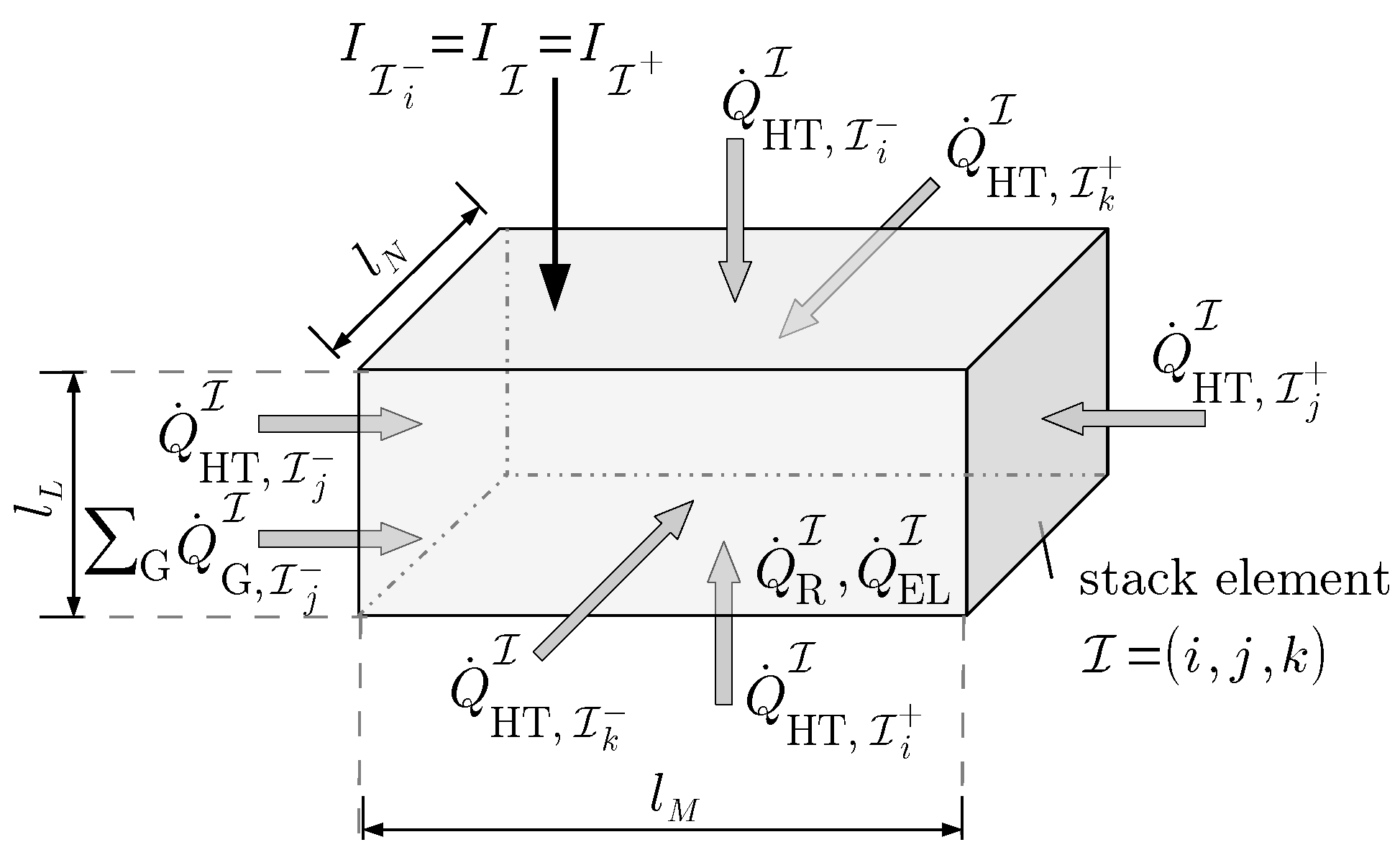
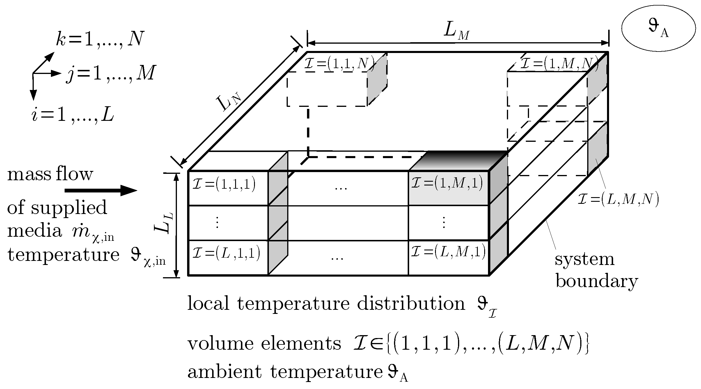
One possibility to derive and implement control and operating strategies that allow for a real-time capable maximization of the electric power production is based on an offline identification of the current–voltage characteristic of the fuel cell. This characteristic can be determined experimentally as a multivariate look-up table depending on a representative temperature in the interior of the fuel cell as well as on the flow rate of hydrogen at the SOFC’s anode inlet manifold.
Already at this point, the definition of the representative temperature of the fuel cell stack is not at all trivial. Due to the distributed parameter behavior of the stack, both spatial and temporal variations of the temperature distribution in the interior of the fuel cell occur—leading to changes in the current–voltage characteristic—if at least one of the heat flows summarized in Figure 1, Figure 2 and Figure 3 changes its value.
These heat flows, entering the balance of internal energy in the fuel cell stack, sketched in terms of a finite-volume semi-discretization in Figure 2, are [9,10,11]:
  • heat transfer Q ˙ HT , J I , J { I i , I i + , I j , I j + , I k , I k + } , due to heat conduction in the interior of the stack as well as internal convection and radiation between the supplied gases m ˙ χ , in and solid components;
  • heat exchange between the stack module and the ambiance, both summarized in the term Q ˙ HT , J I for elements located at the system boundary;
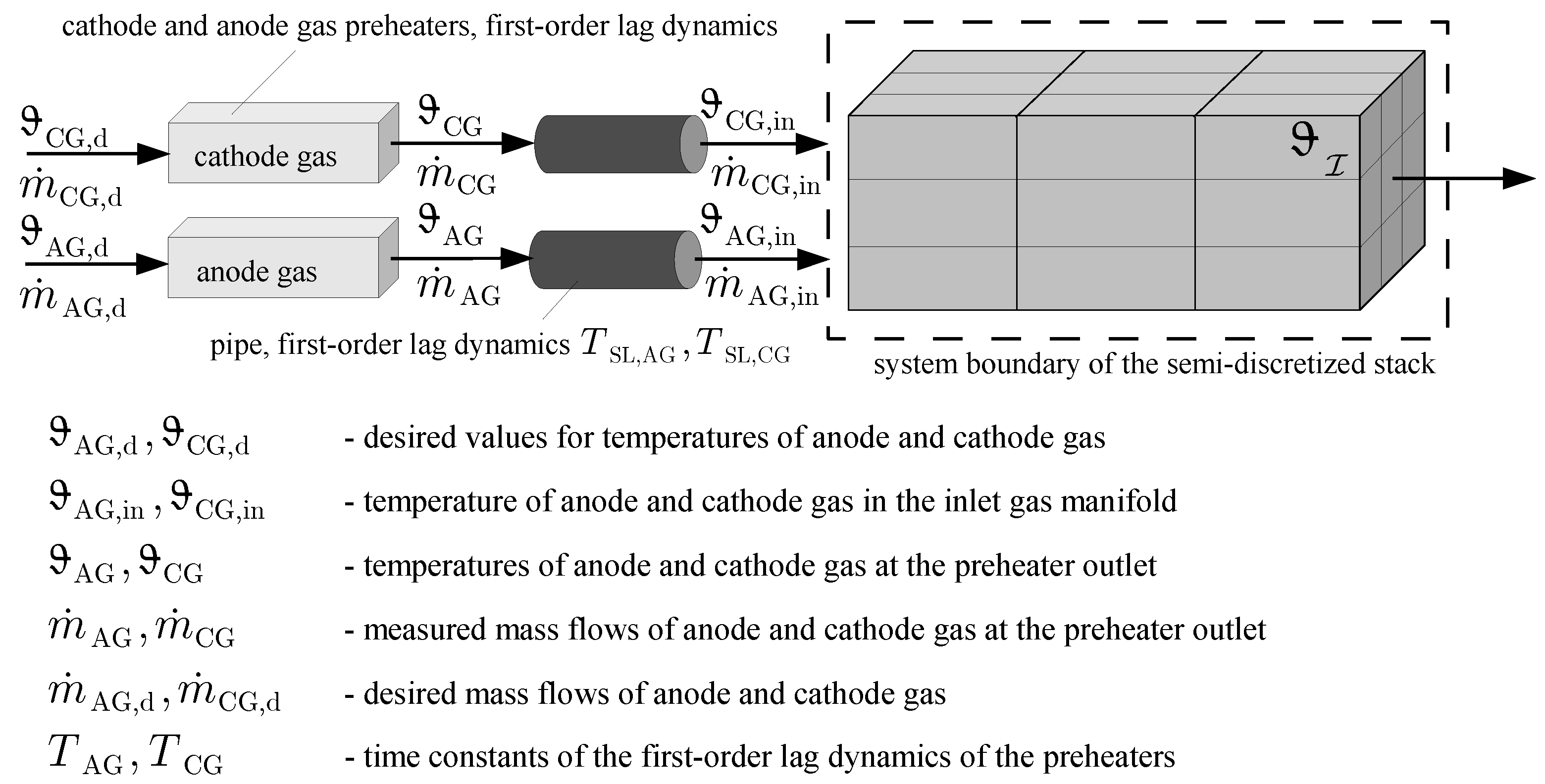
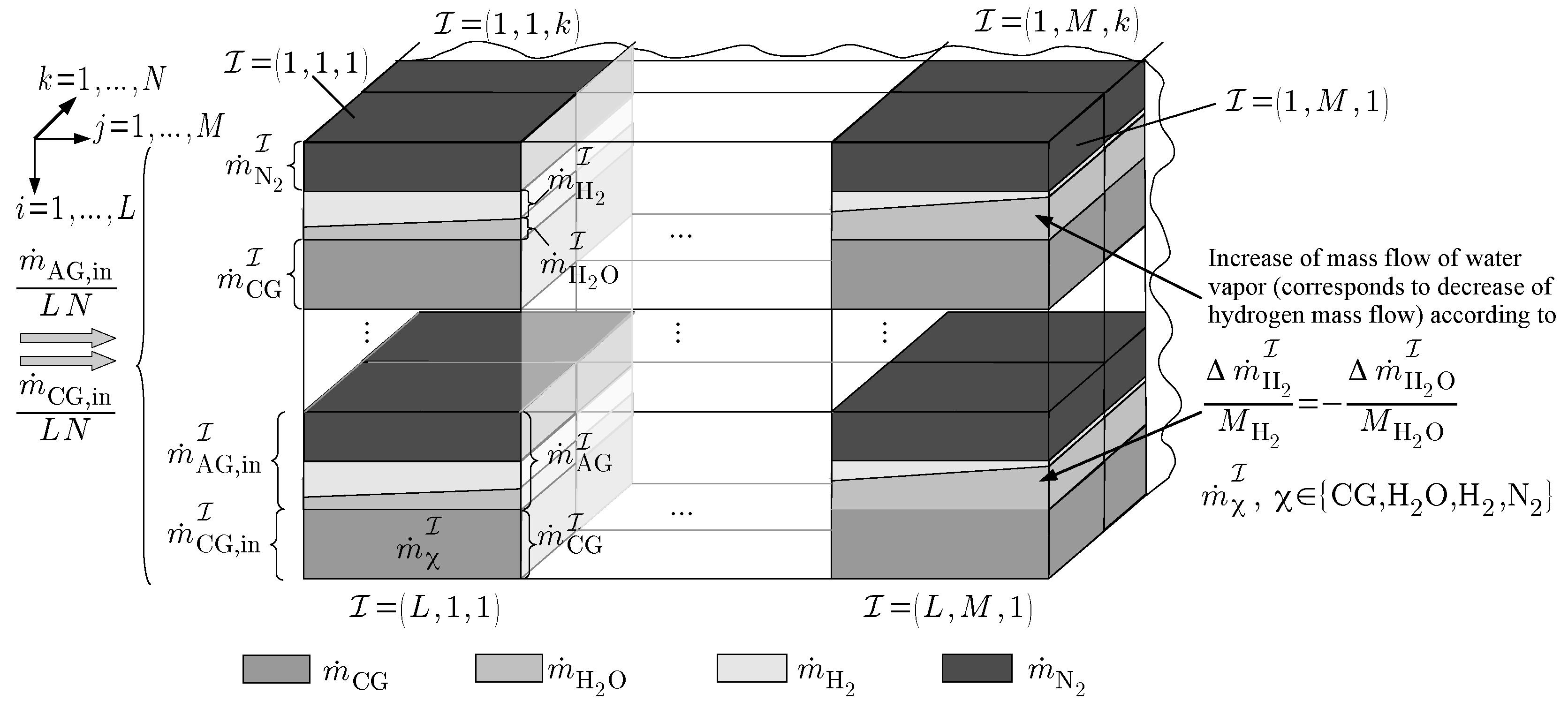
  • enthalpy flows G Q ˙ G , I j I ( t ) , G { AG , CG } , for the anode gas (AG) and the cathode gas (CG);
  • exothermic reaction enthalpies Q ˙ R I ; and
  • Ohmic heat production Q ˙ EL I caused by the internal stack resistance and the local electric currents I I = I M · N , where M · N denotes the number of discretization segments orthogonal to the electric current.
Even if spatially semi-discretized models for the temperature distribution in the fuel cell stack (as those shown in Figure 2 and Figure 3 which were described in detail by Rauh et al. [9]) are reasonable for the implementation of model-based stack temperature estimators and controllers [10,11,12,13,14,15,16], the use of numerous temperature values for the interior of the stack in a semi-discretized manner is not at all practical for the accurate—offline-based—identification of a current–voltage characteristic as a function of each of these thermal state variables. This holds analogously for the spatial variations of the fractions of the anode and cathode gas mass flows, and their respective partial concentrations, which are depicted schematically in Figure 4 for the same semi-discretization that was previously described for the thermal subsystem model.
Therefore, industrial applications typically make use of at most one temperature variable as an influence factor on the electric power characteristic. This variable (for the sake of accessibility for measurements) is commonly chosen as the outlet temperature of the stack (either the anode or cathode gas outlet), which is then also treated as the primary controlled thermal state variable.
Obviously, this value is, on the one hand, corrupted by measurement errors and, on the other hand, cannot fully represent the complete internal state of the stack module. Therefore, each of such offline generated look-up tables (as well as analytic interpolations of these data leading to explicit functional relations) are characterized by unavoidable errors. Especially, they are not capable of capturing the dependency of variable gas inlet manifold temperatures on the steady-state gains between the hydrogen mass flow supplied at the anode and the achievable maximum electric power. However, such kind of dependency was shown experimentally by Frenkel et al. [17] to have a severe influence on the accuracy and stability of electric power control strategies that use the hydrogen mass flow as the primary control variable.
For this reason, this paper proposes to substitute the offline identification of current–voltage and current–power characteristics, respectively, by a real-time capable Kalman filter-based parameter identification. The respective filter is implemented in such a way that a locally quadratic approximation of the electric power as a function of the electric stack current is estimated online during the fuel cell operation in terms of a mean value with corresponding covariance information. This covariance information helps one to quantify the reliability of the estimate and to judge to which precision a maximum power point tracking procedure can work in practice.
Since this Kalman filter solution is based on a locally quadratic approximation, it is only necessary to estimate three parameter values in real time. This reduces memory demands significantly in comparison with multivariate look-up tables and allows for a real-time capable adaptation of the current–power characteristic due to the influence factors described above.
This paper is structured as follows. Section 2 summarizes the fundamental current–voltage as well as current–power characteristics of an SOFC stack module on the basis of measured data of a test rig available at the Chair of Mechatronics at the University of Rostock. Based on an offline identified quasi-static mapping, a simplified quadratic representation of the current–power characteristic is proposed which serves as the basis for a real-time parameter identification. The derivation of a real-time capable Kalman filter for the online parameter identification, replacing classical offline computed quasi-static mappings for the current–power characteristic, concludes this section. Then, a strategy towards a robust maximum power point tracking is proposed in Section 3. The algorithmic properties of both the online parameter identification and maximum power point tracking procedures are investigated in detail by means of real measured data as well as with the help of a simulation case study in this section. Conclusions and an outlook on future work are finally given in Section 4.

2. Kalman Filter Design for Real-Time Estimation of Electric Power Characteristic Of Fuel Cells

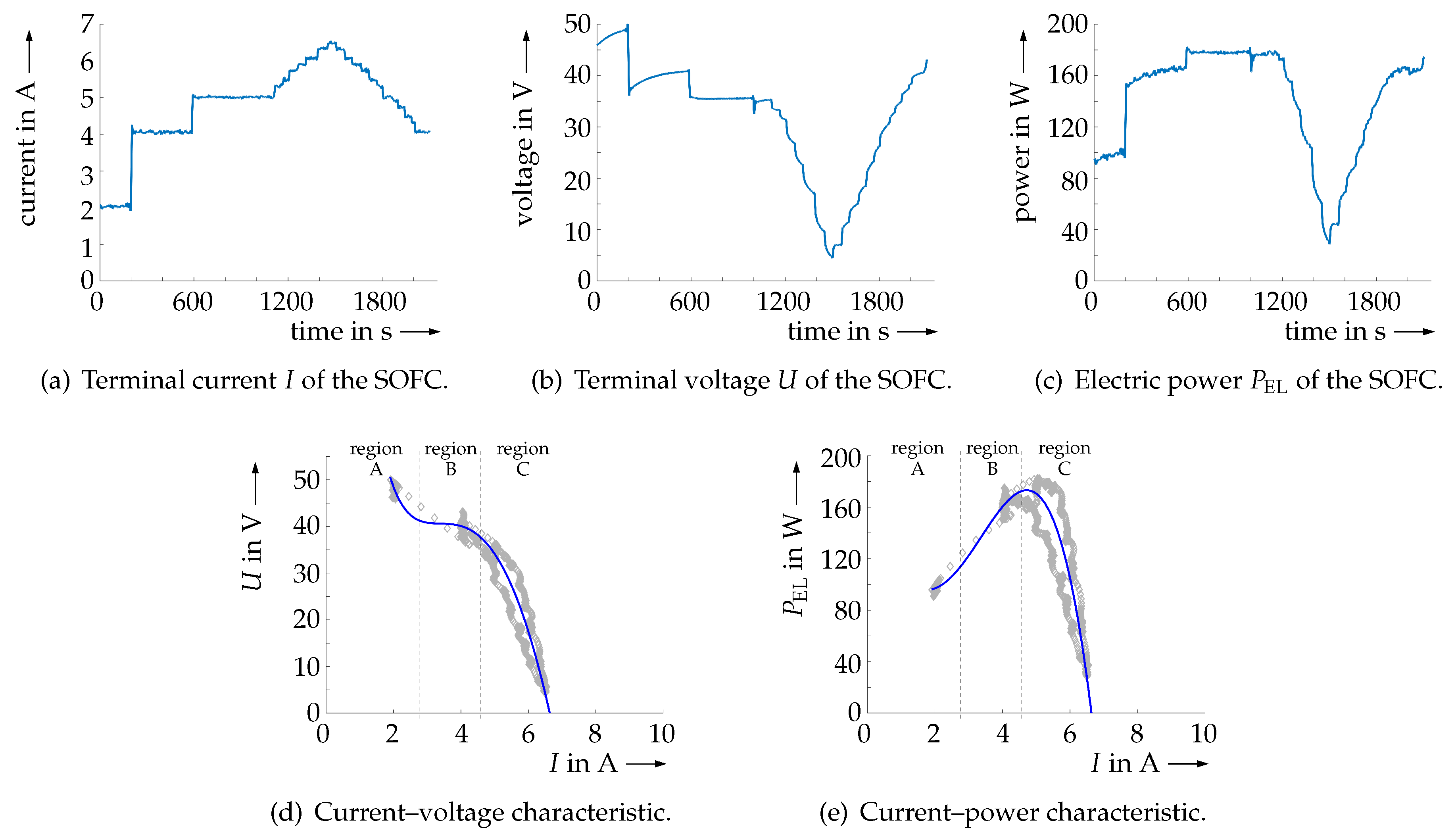
2.1. Fundamental Current–Voltage and Current–Power Characteristics of SOFCs

According to the measured data shown in Figure 5, which were determined for a constant hydrogen mass flow m ˙ H 2 , in 5.1 · 10 6 kg s at the available test rig, the typical dependency between the terminal voltage U of the fuel cell stack and its electric current I (measured at a variable external electric resistance as a load device) becomes clearly visible.
For the presented experiments, an SOFC stack consisting of 60 planar fuel cells in electric series connection was employed. This stack has a maximum electric power output of 1.3 kW . To have sufficient potential for identifying the optimal power point, the stack was operated in part load conditions.
In Figure 5d,e, three different regions can be identified:
  • Region A of activation polarization (characterized by small currents I close to the theoretical Nernst voltage characterizing the SOFC’s open-circuit behavior);
  • Region B of Ohmic polarization corresponding to an almost linear reduction of the terminal voltage for increasing currents I; and
  • Region C of concentration polarization, in which the terminal voltage U rapidly gets close to zero.
After computing the instantaneous electric power according to
P EL , k = U k · I k
at each sampling instant k with the sampling interval t k + 1 t k = 1 s , one can clearly see the existing power maximum in Figure 5e. For the sake of maximizing the electric power production in the following section, it is desirable to identify the maximum of the current–power characteristic in real time, while preventing excessively large currents I coinciding with a negative slope of the current–power characteristic. Such operating points should be avoided in practice by the use of maximum power point tracking approaches because they lead to fuel starvation that can go along with an accelerated degradation of the SOFC module.
Note that maximum power point tracking approaches are well-known also from several other fields of applications. For example, they are extensively used for maximizing the power of photovoltaic systems. However, in recent publications from this area (cf. [18,19]), preventing overshooting the maximum power point is not as crucial as in the SOFC application considered in this paper. Therefore, the approaches applied to photovoltaic systems perform incremental control adaptation schemes without directly accounting for estimation uncertainty in the electric power characteristic. However, for preventing overshooting, this information about uncertainty is essential and can be provided in real time by applying the Kalman filter-based identification scheme derived in this paper.
In Figure 5d,e, analytic approximations, including logarithmic terms inspired by Tafel’s equation [20,21], for the terminal voltage
U k = a 0 + a 1 · I k + a 2 · I k 2 + a 3 · ln I k + a 4 · m ˙ H 2 , in , k + a 5 · I k · m ˙ H 2 , in , k + a 6 · I k · m ˙ H 2 , in , k 2
as well as for the electric power
P EL , k = a 0 + a 1 · I k + a 2 · I k 2 + a 3 · ln I k + a 4 · m ˙ H 2 , in + a 5 · I k · m ˙ H 2 , in , k + a 6 · I k · m ˙ H 2 , in , k 2 · I k
are compared with the measured data under the assumption of a constant hydrogen mass flow. In this case, the parameter estimates listed in Table 1 are obtained, where the coefficients a 4 , a 5 , and a 6 can be set to zero without any loss of information as long as m ˙ H 2 , in , k is constant. Additive offset terms are then fully included in the coefficient a 0 .
This offline identification has been repeated in Figure 6 for larger, temporally slowly varying hydrogen mass flows m ˙ H 2 , in , k at the anode inlet. Again, the same analytic expressions, Equations (2) and (3), were used to compute reasonably accurate approximations. The corresponding numerical parameter values are summarized in Table 2. For both scenarios, they have been computed by a linear least-squares parameter identification similar to the one used in [22] for the dynamics of the electrochemical fuel cell behavior.
For that purpose, Equation (2) has been re-written in the following matrix-vector form
𝓤 K = 𝓓 K · a ,
where the vector
𝓤 K = U 1 U K T
consists of all voltage measurements over a time window k { 1 , , K } , where K denotes a sufficiently large number of (typically a few hundred) measurement points.
In addition, current and mass flow measurements are included in the data matrix
𝓓 K = 1 I 1 I 1 2 ln I 1 m ˙ H 2 , in , 1 I 1 · m ˙ H 2 , in , 1 I 1 · m ˙ H 2 , in , 1 2 1 I K I K 2 ln I K m ˙ H 2 , in , K I K · m ˙ H 2 , in , K I K · m ˙ H 2 , in , K 2 ,
while
a = a 0 a 1 a 2 a 3 a 4 a 5 a 6 T
denotes the parameter vector to be identified. This identification is performed by the classical least-squares solution expressed in terms of
a = 𝓓 K + · 𝓤 K ,
where 𝓓 K + is the left pseudo inverse of the data matrix 𝓓 K according to
𝓓 K + = 𝓓 K T · 𝓓 K 1 · 𝓓 K T .
Note, both experimental datasets and the presented analytic representations for the current–power characteristic are used for validating the filter-based identification and maximum power point tracking procedure in the remainder of this paper. For this maximum power point tracking, it is essential to estimate variations of the current–voltage as well as current–power characteristics in real time, as soon as new measured data become available. This task can be solved partially by classical recursive formulations of least-squares estimation schemes. Suitable references for such approaches can be found in [23]. However, without extensions to a stochastic framework, as presented in the following subsection by means of a Kalman filter synthesis, classical recursive least-squares estimators do not provide information about the accuracy of the coefficient vector a . This issue is solved in this paper by computing the respective (co-)variances of all estimated parameters as described in the following subsection.

2.2. Simplified Model and Kalman Filter Design

To implement an instationary Kalman filter [24,25,26] with the general discrete-time dynamic system model
x k + 1 = A k x k + E k w k
and the measurement equation
y k = C k x k + v k ,
the electric power characteristic of the SOFC is first approximated by a polynomial of order two according to
P EL , k I k 0 I k 1 I k 2 · x k with x k = x 1 , k x 2 , k x 3 , k T R 3
at each time instant t k .
The vector x k (serving as a simplification of the previously introduced parameter vector a ) is treated in the following as the state vector of the Kalman filter to adapt the locally valid quadratic approximation of the current–power characteristic in terms of the available measurements and to account for dependencies of the power curve that are caused by effects other than the current I k . In what follows, the power P EL , k serves as a scalar realization of the general output vector y k .
In general, the Kalman filter for the system model in Equation (10) with Equation (11) consists of the prediction step
μ x , k + 1 p = A k μ x , k e + E k μ w , k
C x , k + 1 p = A k C x , k e A k T + E k C w , k E k T
as well as the measurement-based innovation
μ x , k e = μ x , k p + L k · y ^ k C k μ x , k p μ v , k
C x , k e = C x , k p L k C k C x , k p
with the time-varying Kalman gain
L k = C x , k p C k T C k C x , k p C k T + C v , k 1 .
Here, the noise processes w k and v k are assumed to be given by the stochastically independent normal distributions N ξ , μ ξ , C ξ , ξ w k , v k , ξ R n ξ with
N ξ , μ ξ , C ξ = 1 ( 2 π ) n ξ · det C ξ · exp 1 2 ( ξ μ ξ ) T C ξ 1 ( ξ μ ξ )
and the corresponding mean vectors and covariances μ ξ and C ξ , respectively.
Because the vector x k describing the current–power characteristic of the SOFC is typically slowly varying, the system matrix A k in Equation (10) is set to the identity matrix I 3 × 3 R 3 × 3 in order to represent the neglected system dynamics in terms of a discrete-time integrator disturbance model. In this context, discrete-time integrator disturbance models according to x k + 1 = x k + w k , in which the zero-mean process noise w k is included in additive form, provide an effective means to represent temporally slow variations of the quantities x k , where their typical variability (without any a priori knowledge concerning a preferred direction of change) is expressed by the process noise covariance of w k .
In (10), the process noise w k is assumed to consist of three independent Gaussian noise processes with zero mean μ w , k = 0 with the constant disturbance input matrix E k = I 3 × 3 and the associated diagonal covariance matrix C w , k = diag σ w , 1 2 σ w , 2 2 σ w , 3 2 with the standard deviations σ w , i , i { 1 , 2 , 3 } of the state variability between two subsequent sampling steps.
According to this integrator disturbance model, the predicted parameters of the current–power characteristic can be described by their expected value E x k + 1 = μ x , k + 1 p as well as their covariance matrix C x , k + 1 p according to
μ x , k + 1 p = μ x , k e
C x , k + 1 p = C x , k e + C w , k ,
where all variables denoted with the superscript e refer to the outcome of the previous innovation step. Accounting for the specific structure of the scalar power measurement in Equation (12), the innovation step at the time instant k can be expressed with the help of a zero-mean Gaussian approximation of the power measurement noise (since precise knowledge about the measurement noise variance is crucial for an effective Kalman filter design, it has been determined for the available test rig by means of experiments within the voltage and current measurement range considered in the following investigation) with the variance C v , k . This innovation step precedes the prediction in Equations (19) and (20) and is given by the expectation and covariance update
μ x , k e = μ x , k p + L k · y ^ k I k 0 I k 1 I k 2 · μ x , k p
C x , k e = C x , k p L k · I k 0 I k 1 I k 2 · C x , k p
with the gain vector
L k = C x , k p · I k 0 I k 1 I k 2 · I k 0 I k 1 I k 2 · C x , k p · I k 0 I k 1 I k 2 + C v , k 1 R 3 .
A forecast of the uncertainty in the approximation of the current–power characteristic is based on an evaluation of the respective standard deviation given by
σ P EL , k = E P EL , k E P EL , k 2 = E I k 0 I k 1 I k 2 · x k μ x , k e · x k μ x , k e T · I k 0 I k 1 I k 2 T = I k 0 I k 1 I k 2 · E x k μ x , k e · x k μ x , k e T · I k 0 I k 1 I k 2 T = I k 0 I k 1 I k 2 · C x , k e · I k 0 I k 1 I k 2 T .
This value is used in the following section together with the trace
τ k : = trace C x , k e
of the estimated, strictly positive definite covariance matrix to determine whether the online estimation of the electric power characteristic has already converged sufficiently close to the actual power in the respective operating point so that the approximation in Equation (12) can be used to update the current I k + 1 in a future discretization point. The aim of this update is to attain the maximum power point as closely as possible without overshooting.
Remark 1.
Note, thus far only the dependency of the electric power characteristic on the stack current I k is explicitly included in the real-time identification model. Variations of the (average) stack temperature ϑ FC , k , the anode and cathode gas inlet temperatures ϑ AG , k and ϑ CG , k , and the hydrogen mass flow m ˙ H 2 , in , k are currently treated implicitly in a model-free manner by the time-independent process noise covariance C w , k . To include these further dependencies directly in the identification model, aiming at a recursive stochastic identification, Equation (12) can be replaced straightforwardly by using the matrix Kronecker product in terms of
P EL , k I k m 1 1 m ˙ H 2 , in , k m 2 1 ϑ AG , k m 3 1 ϑ CG , k m 4 1 ϑ FC , k m 5 1 · x ˜ k
with the augmented state vector x ˜ k R i = 1 5 m i . To account for the aforementioned physical dependencies, the vectors
I k m 1 1 = I k 0 I k 1 I k 2 I k m 1 1 ,
m ˙ H 2 , in , k m 2 1 = m ˙ H 2 , in , k 0 m ˙ H 2 , in , k 1 m ˙ H 2 , in , k 2 m ˙ H 2 , in , k m 2 1 ,
ϑ AG , k m 3 1 = ϑ AG , k 0 ϑ AG , k 1 ϑ AG , k 2 ϑ AG , k m 3 1 ,
ϑ CG , k m 4 1 = ϑ CG , k 0 ϑ CG , k 1 ϑ CG , k 2 ϑ CG , k m 4 1 ,
and
ϑ FC , k m 5 1 = ϑ FC , k 0 ϑ FC , k 1 ϑ FC , k 2 ϑ FC , k m 5 1
of monomials of I k , m ˙ H 2 , in , k , ϑ AG , k , ϑ CG , k , and ϑ FC , k need to be included in the extended model in Equation (26) to which the Kalman filter design can be generalized easily.
Remark 2.
To achieve a suitable convergence of the vectors x k (respectively, x ˜ k ) towards a reasonable approximation of the actual current–power dependency, measured data need to be gathered so that the dependency between the variables to be estimated and the electric fuel cell power is sufficiently excited in a persistent form. A corresponding strategy for the fundamental model in Equation (12) is presented in Section 3.

3. Real-time Capable Robust Maximum Power Point Tracking

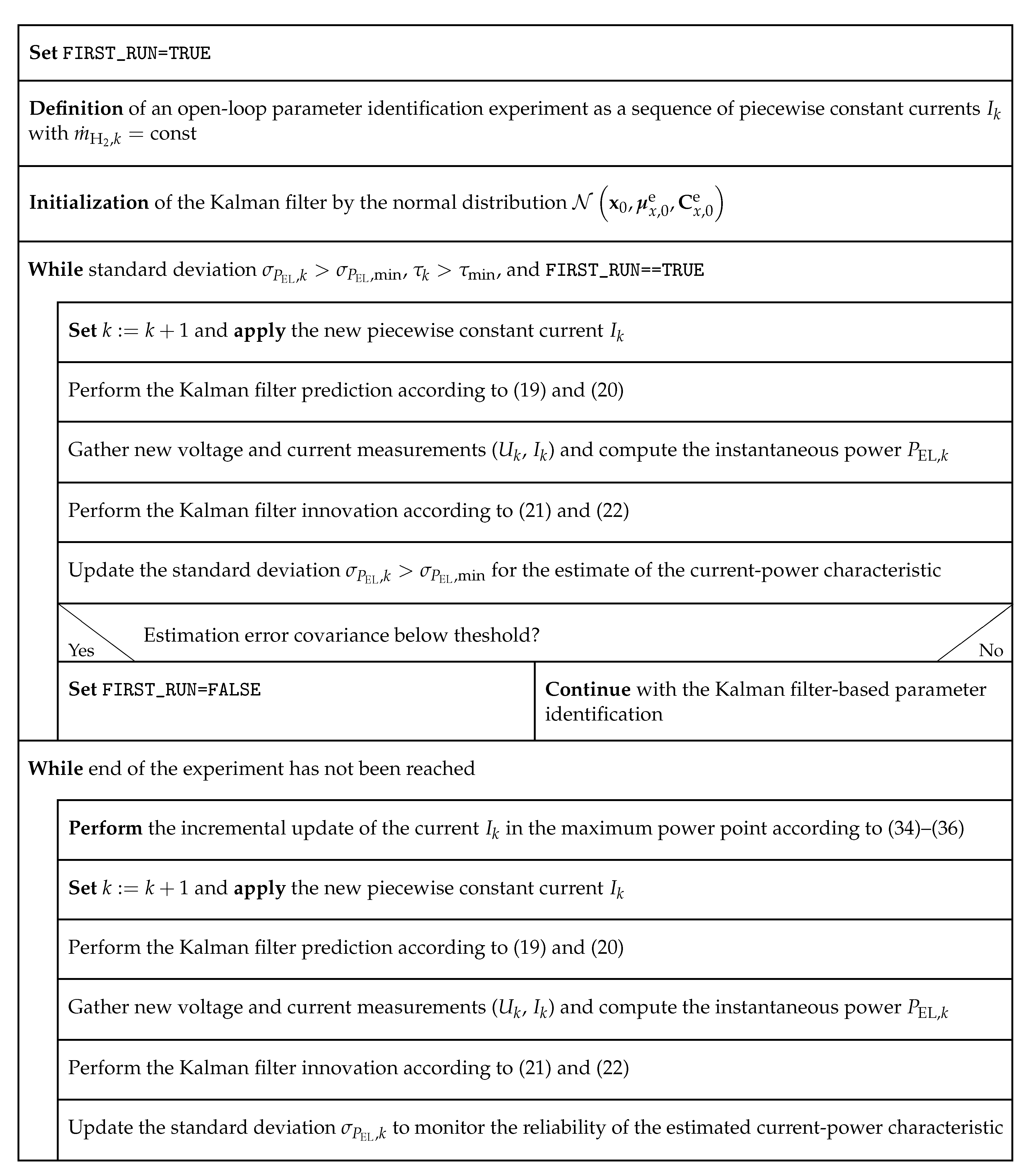
3.1. Algorithm for Combined Parameter Identification and Maximum Power Point Tracking

The proposed algorithm for the real-time capable robust maximum power point tracking summarized in Figure 7 consists of two phases, where only scalar and low-dimensional matrix-vector operations are involved. This leads to computing times that are much smaller than the typical sampling rates of any SOFC controller.
In the first phase, the online identification of the current–power characteristic using the Kalman filter summarized in Section 2 is initialized and executed. For that purpose, a sufficiently rich excitation signal for the electric current is required.
In the scenario under investigation, this input signal is given by a piecewise constant current I k that increases and decreases successively, typically chosen from the desired operating region of Ohmic polarization. In each temporal discretization step, the Kalman filter with the prediction and innovation steps in Equations (19) and (20) as well as Equations (21) and (22), respectively, is evaluated. This open-loop identification is continued up to the point, where the computed standard deviation σ P EL , k falls below the threshold value σ P EL , min for the first time. The same has to hold for the matrix trace τ k defined in Equation (25) to ensure sufficiently small uncertainty in the estimated coefficients of the approximated current–power characteristic in Equation (12).
As soon as this point has been reached, the second phase of the algorithm is initialized. Instead of using a predefined current variation I k , changes in the current now result form an online maximization of the power characteristic. In an uncertainty-free setting, the current I k at the maximum of the power curve in Equation (12) would be given by the necessary optimality condition
P EL , k I k = 0 1 2 I k · x k = 0
leading to the optimal current value
I k = x 2 , k 2 x 3 , k .
However, uncertainty in the estimated parameters x k for the locally approximated current–power characteristic may lead to an undesirable overshoot over the maximum, corresponding to currents in areas in which the power curve has a negative slope. To prevent this phenomenon, the variance estimates for the second and third element of x k are taken into account in the current update according to
I k = μ x , 2 , k e + η · e 2 T · C x , k e · e 2 2 · μ x , 3 , k e η · e 3 T · C x , k e · e 3 ,
where η > 0 represents a user-defined safety margin and e 2 = 0 1 0 T and e 3 = 0 0 1 T . To further smoothen the variation of the current update (avoiding the excitation of non-modeled high-frequency dynamics in the power characteristic violating the assumption of the integrator disturbance model for the system dynamics in Equation (10)), the actual current for the subsequent time step is chosen as the low-pass filtered system input
I k + 1 = I ˜ k + 1 for I ˜ k + 1 I k I k I ˜ k + 1 I k else
with
I ˜ k + 1 = I k + I k I k · e 2 T · C x , k e · e 2 trace C x , k e .
Remark 3.
To guarantee feasible, i.e., non-negative optimized current values I k , the update rule in Equation (34) needs to be parameterized by a suitable combination of η and σ P EL , min such that both inequalities
μ x , 2 , k e + η · e 2 T · C x , k e · e 2 < 0
and
μ x , 3 , k e η · e 3 T · C x , k e · e 3 < 0
are satisfied, while concavity of the approximated current–power characteristic is ensured for each estimate with μ x , 3 , k e < 0 , making Equation (38) satisfied. If possible violations of the condition in Equation (37) are detected during the application of the maximum power point tracking, the computed current I k is rejected and the a priori chosen value of η is reduced by a line search procedure to make the inequality in Equation (37) feasible.
Remark 4.
If the extended system model in Equation (26) is used as a substitute for the quadratic approximation in Equation (12), analytic solutions such as Equation (32) usually no longer exist. The maximization of Equation (26) can then be performed by numerical techniques such as gradient-based or gradient-free extremum seeking approaches [27]. In such cases, real-time capability can be achieved by means of implementations that are based on an online sensitivity analysis (cf. [14,15]).

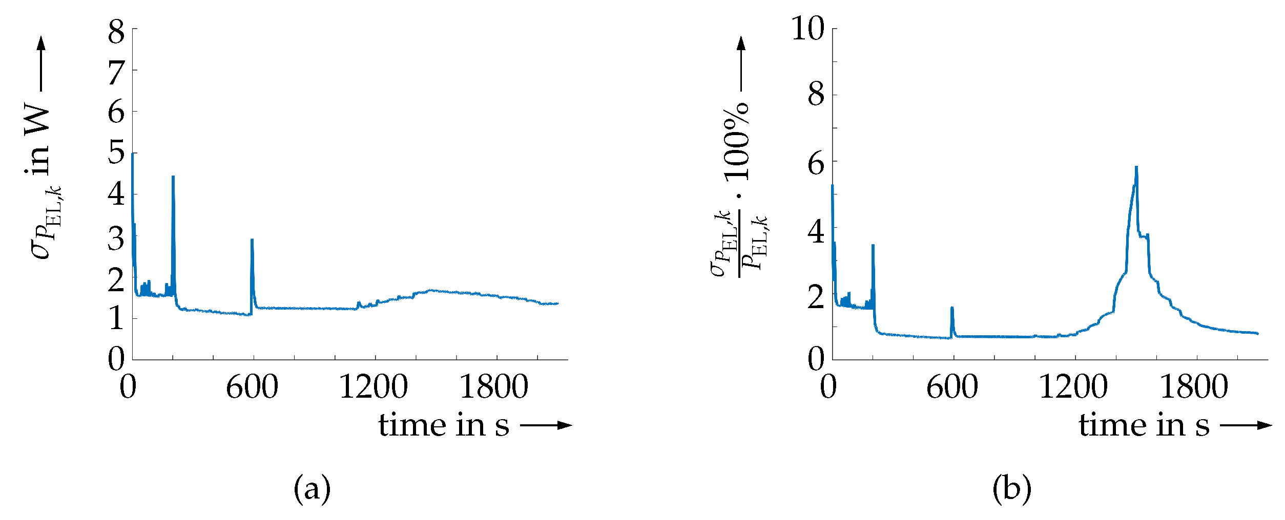
3.2. Kalman Filter-Based Online Parameter Identification

Before results for the real-time capable maximum power point tracking procedure are summarized in the following subsection, the accuracy of the Kalman filter-based online parameter identification was validated. For that purpose, the measured data from Figure 5 were employed. Initially, the vector of expected values μ x , 0 e was chosen as
μ x , 0 e = 501.9 286.1 30.31 T ,
resulting from a second-order Taylor series expansion of Equation (3) at the arbitrarily selected point I = 4.7 A . Due to the large deviation from the initial current I 0 2 A (cf. Figure 5a), the covariance was set to the large initial entries
C x , 0 e = 1 4 · diag μ x , 1 , 0 e 2 μ x , 2 , 0 e 2 μ x , 3 , 0 e 2 .
Despite this significant initial uncertainty and the measurement variance C v , k = 9 W 2 , the approximation for the current–power characteristic converged quickly to the true values, as seen by a comparison of the Kalman filter outputs (the surface in Figure 8) with the measured data as well as with the offline identification result of Figure 5e included in the same graph. Obviously, the Kalman filter provides an accurate second-order polynomial approximation of the true power characteristic at the currently measured data point.
Additionally, the accuracy of the Kalman filter estimates can be quantified with the help of σ P EL , k defined in Equation (24). According to Figure 9, points with the largest uncertainty coincide with those operating conditions at which the step-like current variations depicted in Figure 5a occur. Hence, at those points, the Kalman filter directly provides a hint about the reduced approximation quality of the power curve in the respective situations. Besides a visualization of the absolute values of the estimated standard deviation σ P EL , k in Figure 9a, the percentage σ P EL , k P EL , k · 100 % is shown in Figure 9b to highlight the efficiency of the proposed estimator. Even in transient phases, during which the uncertainty increases inevitably, the relative estimation uncertainty does not exceed the range of 6 % from the currently measured power.

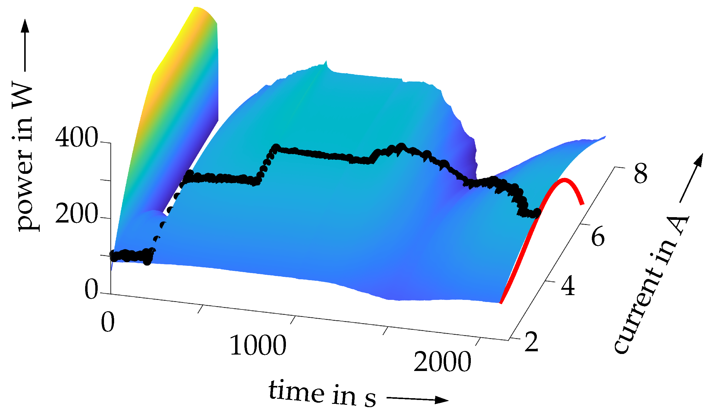
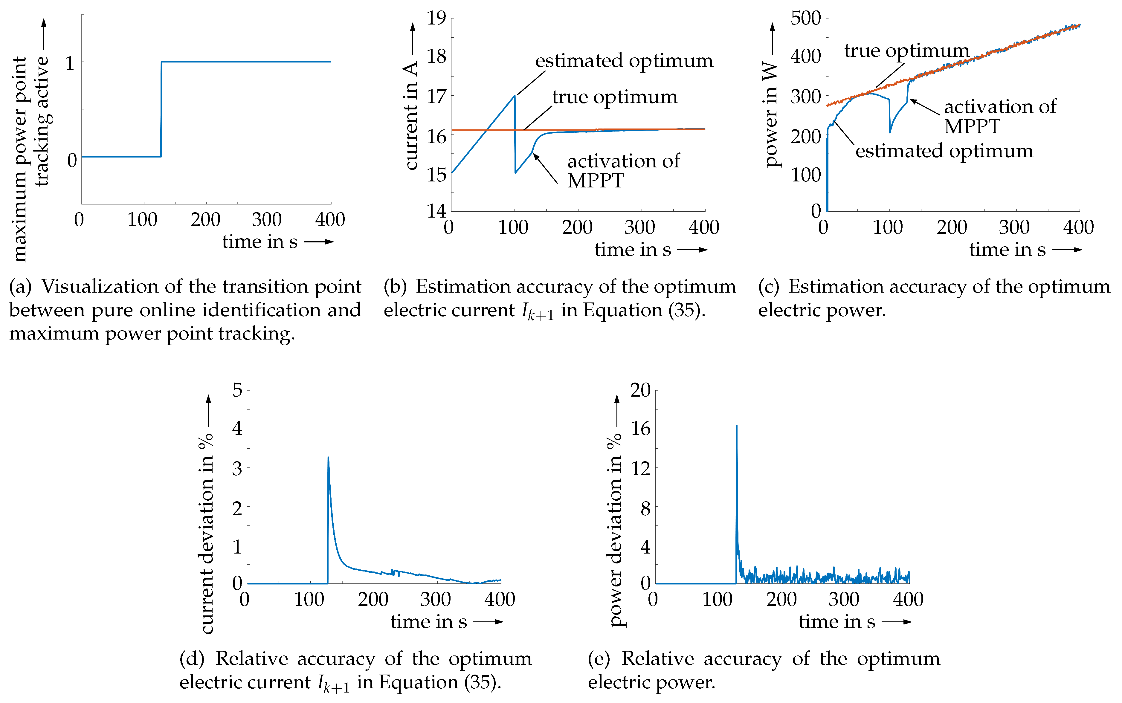
3.3. Numerical Validation of the Maximum Power Point Tracking Procedure

After the capability of the Kalman filter with respect to the accurate online identification of locally quadratic approximations for the current–power characteristic of SOFCs was confirmed, the complete algorithm from Figure 7 was executed. Here, the first phase was based on linearly increasing currents with the upper bound 17 A up to the point where both threshold relations σ P EL , k σ P EL , min , and τ k τ min were satisfied.
According to Figure 10a, this first phase takes approximately 100 discretization steps, if the same initialization as in the previous subsection is used for the Kalman filter. However, to validate the maximum power point tracking capabilities, measured data were now replaced with randomly disturbed values taken from the analytic representation of the current–power map in Figure 6b with a slowly increasing hydrogen mass flow. Both the hydrogen mass flow and the power data were corrupted by zero-mean Gaussian noise with the same standard deviations that appear at the available test rig before they are provided to the estimator and optimization procedure.
As soon as the second phase started (indicated also by arrows in Figure 10b,c, the proposed algorithm allowed for a simultaneous online identification of the power characteristic and for an almost perfect tracking of the optimal operating state. These excellent tracking capabilities are visualized in terms of both the absolute power in Figure 10c and the relative deviations in percent in Figure 10d,e. These figures depict the absolute values of the deviations in percent between the true optima and the corresponding estimates for the electric current and power. Despite the use of noisy data during the maximum power point tracking, the estimation accuracy remained unchanged in comparison with Figure 9, where the pure filter-based identification task was considered.
In this case study, robust overshoot prevention over the maximum power point despite noisy data was achieved by selecting the safety margin η = 0.25 in the optimality condition in Equation (34).

4. Conclusions and Outlook on Future Work

In this paper, a novel Kalman filter-based online identification and maximum power point tracking algorithm is proposed. It was validated experimentally by using measured data from a real-life SOFC test rig. Due to the small computational burden of this algorithm, it is readily applicable to industrial applications and typically outperforms offline identified multivariate look-up table solutions. The advantage of the proposed procedure can not only be seen by its reduced memory demand but also due to the inherent ability to track variations of the power characteristic resulting from instationary thermal and fluidic operating conditions of the SOFC.
Future work will deal with interfacing this estimation and optimization procedure with model-based power control strategies [17]. Moreover, the potential performance increase and resulting robustness of the augmented system representation in Equation (26) will be investigated. The aim of this investigation will be specifically the reduction of the transient first phase of the proposed algorithm with the goal to determine the optimal operating point as quickly as possible.
As mentioned in the Introduction, maximization of the electric power by means of current adaptations, for the case of predefined, or slowly varying hydrogen mass flows is not the only possible optimization task that can be solved by the proposed technique. Future work can also deal with defining an extended cost function, in which the percentage of non-utilized fuel—easily computable by means of Faraday’s law, as shown in [9]—is added in terms of a weighted square norm onto the power to be maximized. Then, using Equation (26) as the augmented system model, it becomes possible to perform a two-parameter optimization task, which determines not only the optimal current for a predefined hydrogen mass flow but allows for optimizing this second input as well. There, it should be assumed that a subsidiary control loop for controlling the hydrogen mass flow exists, either in the case of a direct gas supply (as considered in this paper) or in terms of an external gas reformation process.
Due to its generality, the proposed procedure is not only applicable to the maximization of the electric fuel cell power, but it is also straightforward to transfer this algorithm to any other real-time optimization task on the basis of noisy data, as long as the cost functions under investigation can be identified in terms of expressions that depend linearly on slowly varying estimated parameters as well as have a unique, regular extremum in the interior of the admissible operating domain.

Author Contributions

Conceptualization, A.R.; Methodology, A.R.; Software, A.R.; Validation, A.R., W.F. and J.K.; Investigation, A.R., W.F. and J.K.; Writing—original draft preparation, A.R., W.F. and J.K.; Writing—review and editing, A.R., W.F. and J.K.; Visualization, A.R., W.F. and J.K.; Project administration, A.R.; Funding acquisition, A.R. All authors have read and agreed to the published version of the manuscript.

Funding

This research is partially funded by the European Union within the European Fund for Regional Development.

Conflicts of Interest

The authors declare no conflict of interest.

References

  1. Huang, B.; Qi, Y.; Murshed, A.K.M.M. Dynamic Modeling and Predictive Control in Solid Oxide Fuel Cells: First Principle and Data-based Approaches; John Wiley & Sons: Chichester, UK, 2013. [Google Scholar]
  2. Huang, B.; Qi, Y.; Murshed, A.K.M.M. Solid Oxide Fuel Cell: Perspective of Dynamic Modeling and Control. J. Process Contr. 2011, 21, 1426–1437. [Google Scholar] [CrossRef]
  3. Stiller, C.; Thorud, B.; Bolland, O.; Kandepu, R.; Imsland, L. Control Strategy for a Solid Oxide Fuel Cell and Gas Turbine Hybrid System. J. Power Sourc. 2006, 158, 303–315. [Google Scholar] [CrossRef]
  4. Dicks, A.L.; Rand, D.A.J. Fuel Cell Systems Explained; John Wiley & Sons: Chichester, UK, 2018. [Google Scholar]
  5. Gubner, A. Non-Isothermal and Dynamic SOFC Voltage-Current Behavior. In Solid Oxide Fuel Cells IX (SOFC-IX): Volume 1—Cells, Stacks, and Systems; Singhal, S.C., Mizusaki, J., Eds.; The Electrochemical Society: Pennington, NJ, USA, 15–20 May 2005; pp. 814–826. [Google Scholar]
  6. PEM Fuel Cell. Available online: www.psenterprise.com/sectors/fuelcell (accessed on 2 March 2020).
  7. Pukrushpan, J.; Stefanopoulou, A.; Peng, H. Control of Fuel Cell Power Systems: Principles, Modeling, Analysis and Feedback Design; Springer: Berlin, Germany, 2005. [Google Scholar]
  8. Bove, R.; Ubertini, S. Modeling Solid Oxide Fuel Cells; Springer: Berlin, Germany, 2008. [Google Scholar]
  9. Rauh, A.; Senkel, L.; Kersten, J.; Aschemann, H. Reliable Control of High-Temperature Fuel Cell Systems using Interval-Based Sliding Mode Techniques. IMA J. Math. Contr. Inform. 2016, 33, 457–484. [Google Scholar] [CrossRef]
  10. Rauh, A.; Senkel, L.; Aschemann, H. Interval-Based Sliding Mode Control Design for Solid Oxide Fuel Cells with State and Actuator Constraints. IEEE Trans. Ind. Electron. 2015, 62, 5208–5217. [Google Scholar] [CrossRef]
  11. Rauh, A.; Senkel, L.; Aschemann, H. Reliable Sliding Mode Approaches for the Temperature Control of Solid Oxide Fuel Cells with Input and Input Rate Constraints. In Proceedings of the 1st IFAC Conference on Modelling, Identification and Control of Nonlinear Systems MICNON 2015, St. Petersburg, Russia, 24–26 June 2015. [Google Scholar]
  12. Rauh, A.; Senkel, L.; Auer, E.; Aschemann, H. Interval Methods for the Implementation of Real-Time Capable Robust Controllers for Solid Oxide Fuel Cell Systems. Math. Comput. Sci. 2014, 8, 525–542. [Google Scholar] [CrossRef]
  13. Rauh, A.; Senkel, L. Interval Methods for Robust Sliding Mode Control Synthesis of High-Temperature Fuel Cells with State and Input Constraints. In Variable-Structure Approaches: Analysis, Simulation, Robust Control and Estimation of Uncertain Dynamic Processes; Rauh, A., Senkel, L., Eds.; Springer: Cham, Switzerland, 2016; pp. 53–85. [Google Scholar]
  14. Rauh, A.; Senkel, L.; Aschemann, H. Sensitivity-Based State and Parameter Estimation for Fuel Cell Systems. IFAC Proceedings Volumes 2012, 45, 57–62. [Google Scholar] [CrossRef]
  15. Senkel, L.; Rauh, A.; Aschemann, H. Experimental Validation of a Sensitivity-Based Observer for Solid Oxide Fuel Cell Systems. In Proceedings of the 18th International Conference on Methods & Models in Automation & Robotics (MMAR), Międzyzdroje, Poland, 26–29 August 2013. [Google Scholar]
  16. Kunusch, C.; Puleston, P.; Mayosky, M. Sliding-Mode Control of PEM Fuel Cells; Springer: London, UK, 2012. [Google Scholar]
  17. Frenkel, W.; Rauh, A.; Kersten, J.; Aschemann, H. Experiments-Based Comparison of Different Power Controllers for a Solid Oxide Fuel Cell Against Model Imperfections and Delay Phenomena. Algorithms 2020, in press. [Google Scholar]
  18. Kumar, N.; Hussain, I.; Singh, B.; Panigrahi, B.K. Framework of Maximum Power Extraction From Solar PV Panel Using Self Predictive Perturb and Observe Algorithm. IEEE Trans. Sustain. Energ. 2018, 9, 895–903. [Google Scholar] [CrossRef]
  19. Li, C.; Chen, Y.; Zhou, D.; Liu, J.; Zeng, J. A High-Performance Adaptive Incremental Conductance MPPT Algorithm for Photovoltaic Systems. Energies 2016, 9, 288. [Google Scholar] [CrossRef] [Green Version]
  20. Burstein, G. A Hundred Years of Tafel’s Equation: 1905–2005. Corrosion Sci. 2005, 47, 2858–2870. [Google Scholar] [CrossRef]
  21. Tafel, J. Über die Polarisation bei kathodischer Wasserstoffentwicklung. Zeitschrift für physikalische Chemie 1905, 50, 641–712. (In German) [Google Scholar] [CrossRef]
  22. Frenkel, W.; Rauh, A.; Kersten, J.; Aschemann, H. Optimization Techniques for the Design of Identification Procedures for the Electro-Chemical Dynamics of High-Temperature Fuel Cells. In Proceedings of the 24th IEEE Intl. Conference on Methods and Models in Automation and Robotics (MMAR), Międzyzdroje, Poland, 26–29 August 2019. [Google Scholar]
  23. Isermann, R.; Münchhof, M. Identification of Dynamic Systems: An Introduction with Applications; Springer: Heidelberg, Germany, 2011. [Google Scholar]
  24. Kalman, R.E. A New Approach to Linear Filtering and Prediction Problems. J. Basic Eng. 1960, 82, 35–45. [Google Scholar] [CrossRef] [Green Version]
  25. Stengel, R. Optimal Control and Estimation; Dover Publications: Mineola, NY, USA, 1994. [Google Scholar]
  26. Anderson, B.; Moore, J. Optimal Filtering; Dover Publications: Mineola, NY, USA, 2005. [Google Scholar]
  27. Nocedal, J.; Wright, S. Numerical Optimization; Springer: Berlin, Germany, 2006. [Google Scholar]
Figure 1. Semi-discretization of the fuel cell stack module with gas preheaters.
Algorithms 13 00058 g001
Figure 2. Spatial semi-discretization of the fuel cell stack module.
Algorithms 13 00058 g002
Figure 3. Local energy balance of the semi-discretized fuel cell stack module.
Algorithms 13 00058 g003
Figure 4. Local mass flow balances in the semi-discretized fuel cell stack module.
Algorithms 13 00058 g004
Figure 5. Measured electric current I, terminal voltage U, and electric power P EL of the SOFC for a relatively small, constant hydrogen mass flow m ˙ H 2 , in 5.1 · 10 6 kg s .
Algorithms 13 00058 g005
Figure 6. Offline identification of the current–voltage and current–power characteristic for larger, temporally varying hydrogen mass flows m ˙ H 2 , in . (a) Fuel cell voltage depending on the terminal current and hydrogen mass flow. (b) Fuel cell power depending on the terminal current and hydrogen mass flow.
Algorithms 13 00058 g006
Figure 7. Structure diagram of the Kalman filter-based parameter identification and maximum power point tracking.
Algorithms 13 00058 g007
Figure 8. Kalman filter-based online parameter identification for the measured data in Figure 5a–c; black dots represent the power measurements in Figure 5c; the red curve at the final time instant corresponds to the offline identified current–power characteristic in Figure 5e.
Algorithms 13 00058 g008
Figure 9. Quantification of the accuracy of the estimated electric fuel cell power. (a) Standard deviation of the estimated power. (b) Deviation of the estimated power in percent.
Algorithms 13 00058 g009
Figure 10. Validation of the Kalman filter-based maximum power point tracking procedure; relative deviations in Figure 10d,e are only reasonable for the phase in which the maximum power point tracking (MPPT) is active. In inactive phases, they are purposefully set to zero.
Algorithms 13 00058 g010
Table 1. Offline identified parameters of the current–voltage and current–power characteristics as a function of the stack current I k for constant hydrogen mass flow m ˙ H 2 , in , k 5.1 · 10 6 kg s in Figure 5d,e.
ParameterValue
a 0 23.3553
a 1 135.3495
a 2 10.0203
a 3 229.1167
a 4 0
a 5 0
a 6 0
Table 2. Offline identified parameters of the current–voltage and current–power characteristics as a function of the stack current I k and the hydrogen mass flow m ˙ H 2 , in , k .
ParameterValue
a 0 1.38 · 10 4
a 1 1.13 · 10 3
a 2 1.603 · 10 1
a 3 9.977 · 10 3
a 4 1.926 · 10 7
a 5 5.475 · 10 5
a 6 5.198 · 10 3

