On a Hybridization of Deep Learning and Rough Set Based Granular Computing


Faculty of Mathematics and Computer Science, University of Warmia and Mazury in Olsztyn, 10-710 Olsztyn, Poland
*
Author to whom correspondence should be addressed.
Algorithms 2020, 13(3), 63; https://0-doi-org.brum.beds.ac.uk/10.3390/a13030063
Submission received: 20 February 2020
/
Revised: 6 March 2020
/
Accepted: 7 March 2020
/
Published: 11 March 2020
(This article belongs to the Special Issue Algorithms for Pattern Recognition)
Abstract
:The set of heuristics constituting the methods of deep learning has proved very efficient in complex problems of artificial intelligence such as pattern recognition, speech recognition, etc., solving them with better accuracy than previously applied methods. Our aim in this work has been to integrate the concept of the rough set to the repository of tools applied in deep learning in the form of rough mereological granular computing. In our previous research we have presented the high efficiency of our decision system approximation techniques (creating granular reflections of systems), which, with a large reduction in the size of the training systems, maintained the internal knowledge of the original data. The current research has led us to the question whether granular reflections of decision systems can be effectively learned by neural networks and whether the deep learning will be able to extract the knowledge from the approximated decision systems. Our results show that granulated datasets perform well when mined by deep learning tools. We have performed exemplary experiments using data from the UCI repository—Pytorch and Tensorflow libraries were used for building neural network and classification process. It turns out that deep learning method works effectively based on reduced training sets. Approximation of decision systems before neural networks learning can be important step to give the opportunity to learn in reasonable time.
1. Introduction
This paper is divided into parts dedicated to deep learning, rough sets, granular computing by means of rough mereology. Deep learning as a collection of techniques and is rooted in artificial neural networks (ANN’s) [1,2,3]. The idea of a neural network is that of an acyclic directed graph whose nodes are computing units—neurons—joined by edges labelled with weights. Nodes with input degrees of zero are called inputs while nodes with the output degree zero are said to be outputs. The flow of information is forward: from input nodes to output nodes. Nodes are classified into layers, each layer defined recurrently starting from the input nodes layer. Exemplary Computation by a neural net begins with the input vector and in the simple case of a sigmoidal perceptron, with the input x, the output is given as , f being an activation sigmoidal function. The result of the computation is the vector output by the output layer of neurons.
The learning procedure for ANN’s is a series of computations on sequences of training vectors which stops when the output vector is sufficiently close to the target vector on each input vector. Theoretically justified by the Perceptron Learning Theorem [4], the method of learning by changing weights by the delta rule turned effective when the backpropagation technique came into usage [5]. Deep learning proceeds further by enhancing the neural net with many filters allowing for exhibiting of many local features. Some variants like LSTM allow for reaching deep back into memory of the process which makes such networks especially effective in, for example, speech processing [6]. For a general introduction please consult [7].
Interesting research on the field of granular computation with the use of neural network techniques can be found in the works [8,9,10]. To the best of our knowledge, there is no similarity to our research in this context, so direct comparison is difficult. In addition, the aim of our work is to check whether the data prepared by our granulation techniques are learned through deep neural networks. It is not our goal to show that we have the best technique to reduce training systems.
Rough set theory [11] approaches data in set-theoretical terms by assuming that on each collection of vectors representing some objects, a partition is obtained, its classes representing distinct concepts/categories pertaining to those objects. A general concept, i.e., a set of objects in a given collection (the universe) is perceived through categories: some concepts can be expressed by categories in a deterministic way and some may not. The former are exact concepts (modulo the given partition into categories) while the latter are inexact (rough) concepts. Each rough concept can only be expressed in terms of its relation to categories by approximations: the lower approximation of a concept consists of categories (or, exact concepts) contained in the concept whereas the upper approximation consists of categories intersecting the given concept.
A means for dealing with data is provided by the notion of an information system (see Pawlak, op.cit.) which is a tuple where U is a universe of objects, A is a set of attributes, V is a set of attribute values, and, f is a mapping which assigns to each object and each attribute , the value . Categories obtained in this case are classes of the indiscernibility relation for each , where B is a subset of the set A of attributes. A special case of information systems is a decision system with signature where d is a new attribute not in A, called the decision. A relation between sets and for some B is called a decision algorithm over B. For algorithmic methods of inducing decision rules please see [12,13]. A far reaching extension of rough set theory is rough mereology [14]. Rough mereology applies as its primitive notion that of a part to a degree [15]. Parts to a degree are subjected to a few basic restrictions which reflect properties of partial containment: each object is a part to itself to the degree of 1, if an object x is a part to a degree of 1 to an object y then for each object z, the degree to which z is contained in x is not greater than the degree to which z is contained in y. Rough mereology in turn was applied in a formal definition of granules of knowledge [16,17]. Formally, given a measure m of partial containment (called in Polkowski-Skowron a rough inclusion), a granule of the radius r about an object x is the collection of all objects which are parts of x to degrees of at least r. Consult [15] for a deeper discussion of computing with granules. On the basis of computing with rough mereological granules, an approach to data mining was proposed [16]. This approach consists in transforming a given decision system (data set) into a granular decision system where: G is a set of granules of radius r about objects in U which provides a covering of U; is a set of attributes for , each maps each granule g into the value set V according to the formula where S is a selected strategy like e.g., majority voting with random tie resolution; V is the value set unchanged; ; is defined in the same manner as . To the granular decision system any standard algorithm for rule induction can be applied for all plausible values of the radius r. This ends our introduction of the main ingredients in our approach. In the following sections, we give details of our approach and we present results.
In the work we are focusing on deep learning effectiveness on the reduced decision systems, we check the level of internal knowledge maintenance in terms of classification effectiveness.
2. Reducing the Size of Decision-Making Systems Based on Their Granular Reflections
As a reference technique, we have chosen one of our best methods for the approximation of decision systems (concept-dependent granulation), which works analogously to the baseline procedure described in this section, while granule formation takes place separately within decision classes.
Granulation consists in reducing the size of the training decision-making system through the process of creating granular reflections of data.
The definition of the concept-dependent granule formulation is in the Section 2.2.
Let’s move on to the basic technique. Our methods are based on rough inclusions. Introduction to rough inclusions in the framework of rough mereology is available in [16,18]; a detailed, extensive discussion can be found in [15].
In the Polkowski’s granulation procedure, we can distinguish three basic steps.
- First step: granulation. We begin with computation of granules around each training object using selected method. In the method used in this article, by surrounding the objects of the training system class with objects indiscernible to the degree determined by the granulation radius.
- Second step: the process of covering. The training decision system is covered by selected granules. After the calculation of granules in point 1, a group of granules that cover the entire training system with their objects is searched for.
- Third step: building the granular reflections. The granular reflection of original training decision system is derived from the granules selected in step 2. We form new objects by converting granules using majority voting.
We start with detailed description of the basic method—see [16].
2.1. Standard Granulation
For the sake of simplicity we use the following definition of decision system, it is triple , where U is the universe of objects, A the set of conditional attributes, is the decision attribute, and granulation radius from the set {}.
The standard rough inclusion , for and for selected is defined as
where
For each object , and selected , we compute the standard granule as follows,
In the next step we use selected strategy to cover the training decision set U by computed granules—the random choice is the simplest among the most effective studied in [19]). All studied methods are available in [19] (pp. 105–220).
In the last step, granular reflection of training decision set is computed with use of Majority Voting procedure. The ties are resolved randomly.
The process of granulation can be tuned with help of the triangular part of granular indiscernibility matrix , where
2.2. Concept Dependent Granulation
A concept-dependent (cd) granule of the radius about u is defined as follows:
2.2.1. Toy Example of Concept Dependent Granulation
For the decision system from Table 1, we have found concept-dependent granules.
For the granulation radius , the granular concept-dependent indiscernibility matrix (gcdm) is shown in Table 2.
Hence, the granules in this case are
Considering the random choice, the covering can be .
The concept dependent granular decision system formed from coverage is in Table 3.
The majority voting was applied only into the granule .
3. Design of the Experimental Part
A general scheme of the experimental part design is shown in in Figure 1. The neural network architecture was chosen experimentally. For each tabular dataset used we have run our experiment using the same network architecture to make it more comparable. We conducted 10 series of tests for each system tested. Since the data sets used are small in size, we have built a network with simple architecture. In addition, we have selected sets that have two decision classes at the output. In subsequent experiments, the diversity of sets will be increased.
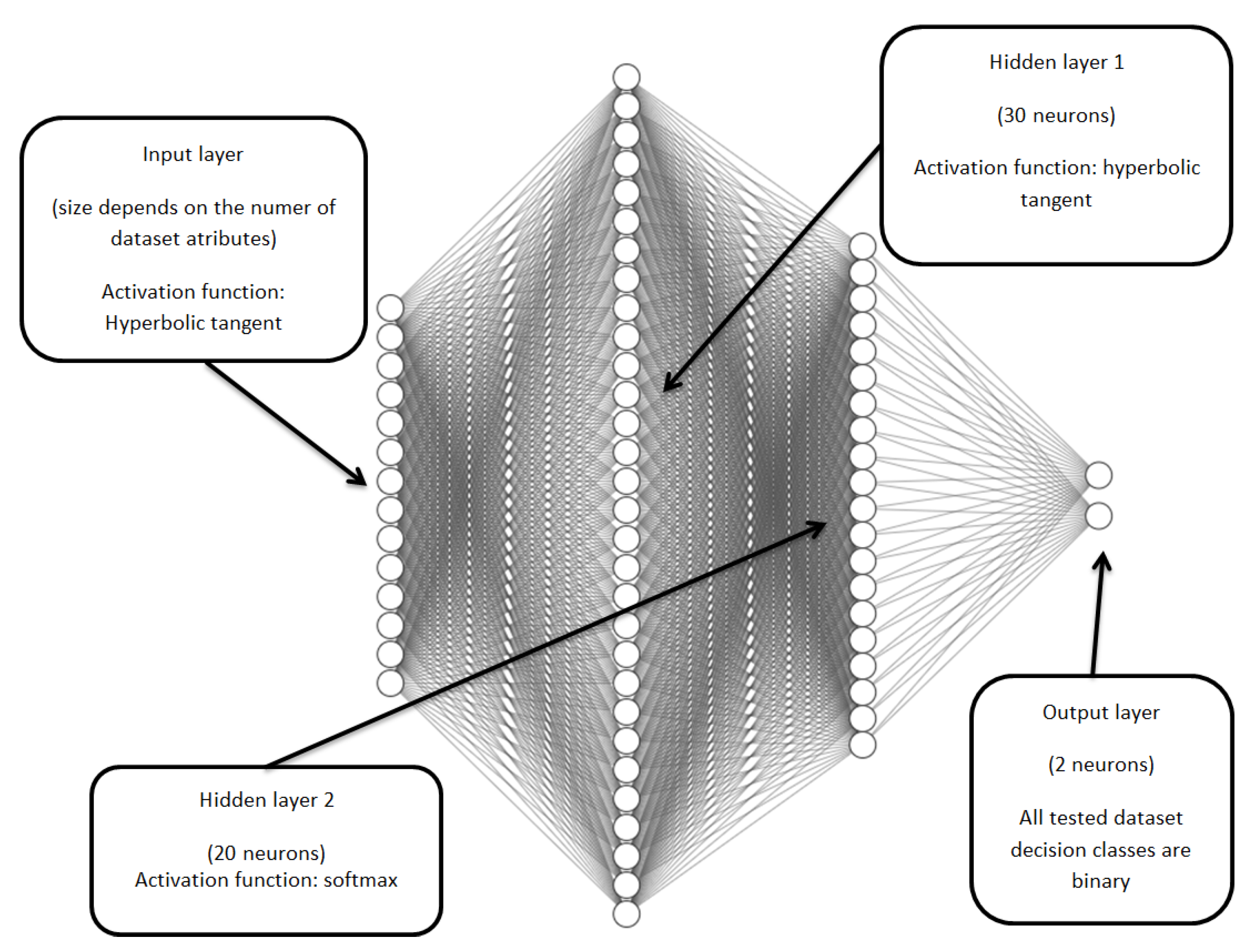
Our network consists of an input layer, two hidden linear layers and an output layer. Input layer is the only layer which size is dynamical and depends on the dataset used. First hidden layer consists of 30 neurons and the second one of 20 neurons. Output layer consists of only two neurons as the decision classes are binary in all used datasets.
We used a hyperbolic tangent as an activation function in layer 1 and 2 and a softmax function in layer number 3. Our network is using an Adam optimizer and a learning rate equal to . To calculate the value of the loss function Cross Entropy was used. Each iteration is being performed across 500 epochs.
4. Procedure for Performed Experiments
General scheme of the test carried out and detail neural network architecture we have on the Figure 1 and Figure 2. Let us present below the combined procedure of our experiments.The procedure of experimentation:
- 1.
- Data input (original decision system),
- 2.
- Data random split in the ratio 70-30 per cent TRN-TST,
- 3.
- Granulation step, covering step, new objects generation—see Section 2.2.1,
- 4.
- Neural network learning step for each set of objects (for each granulation radius) see Figure 1,
- 5.
- Classification step for each test set, based on approximated data see Figure 2,
- 6.
- Compute accuracy, time, number of objects and compare vs first set. The whole procedure is repeated 10 times.
The Results of Experiments
In this section we show the exemplary results for our selected technique, to show the effectiveness of deep learning in classification based on reduced training data. We have the results for Monte Cross Validation 10 method for selected data sets (see Table 4) from UCI repository [20].
The internal knowledge from the original training decision systems—measured by ability for classification—seems to be preserved in sufficient way (the accuracy of classification is comparable with nil case, without reduction). The nil case is for radius 1.
The results of the experiments showed the usefulness of learning neural networks on granular data.
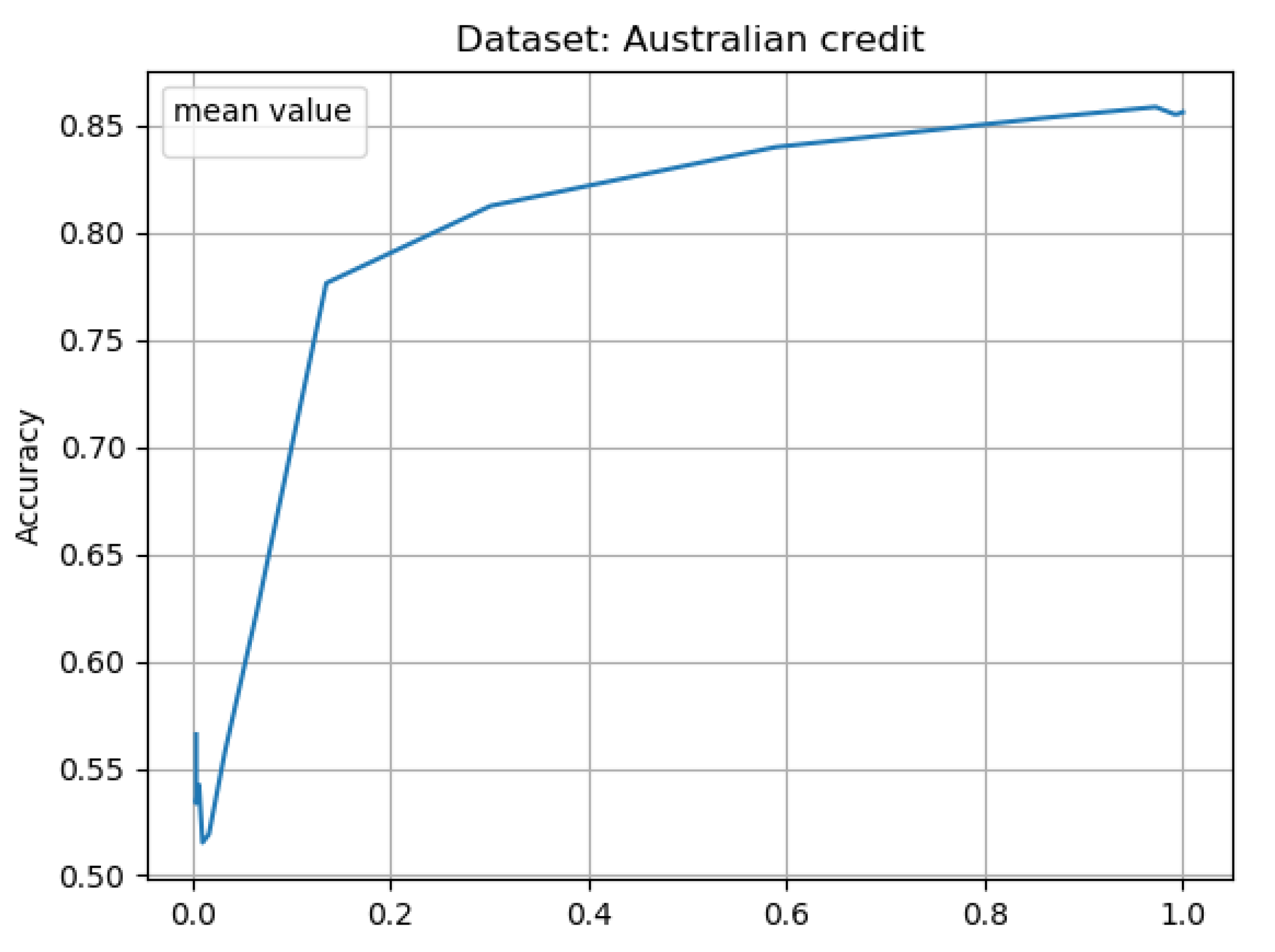
Additionally to accuracy of classification vs the percentage of training size (the size after granulation) for 10 iteration of learning (see Figure 3, Figure 5, Figure 7 and Figure 9)—we have presented average results from 10 experiments considering as x ax the radii of granulation (see Figure 4, Figure 6, Figure 8 and Figure 10). The latter result visualizes the classification accuracy results presented in the Table 5, Table 6, Table 7 and Table 8.
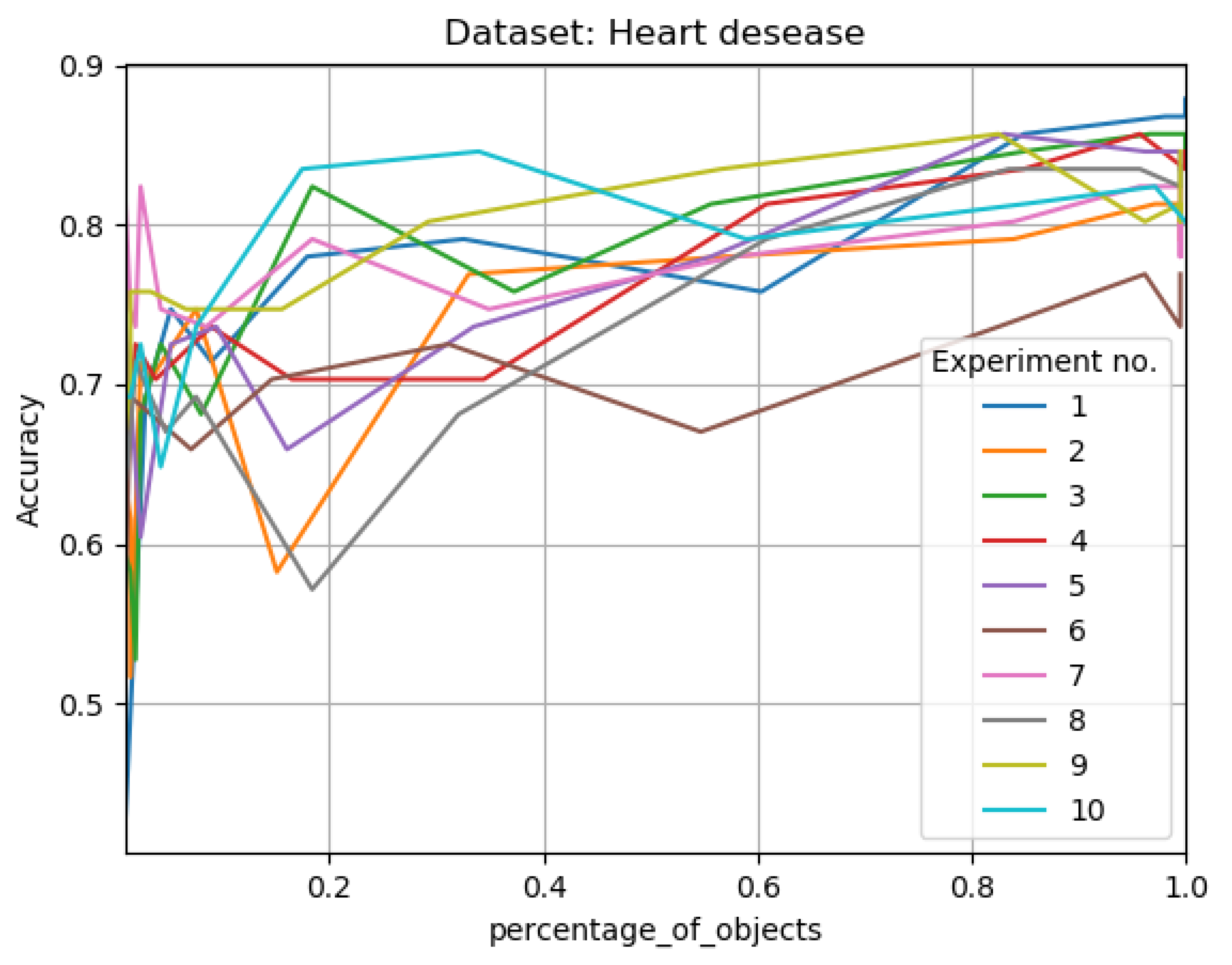
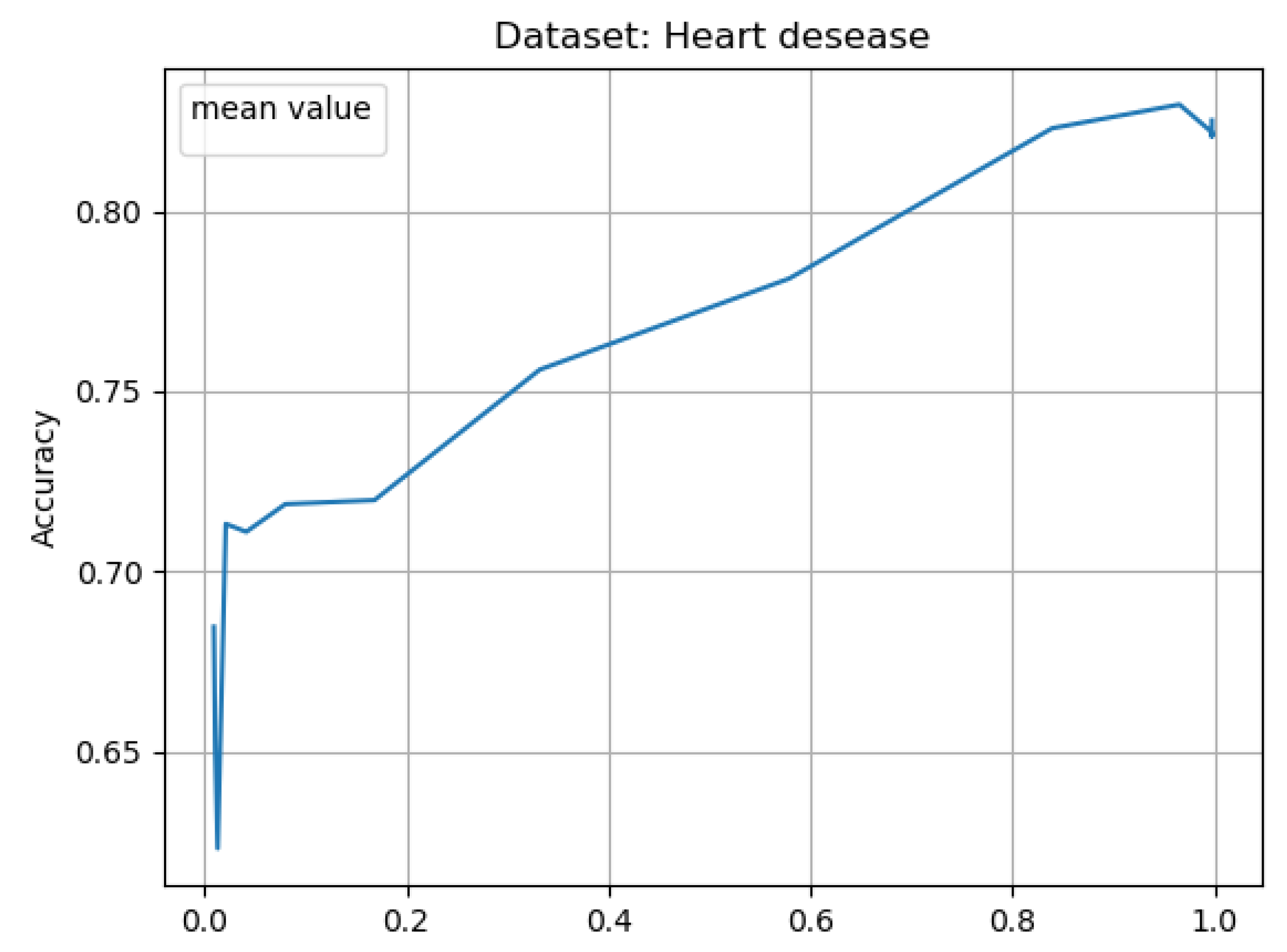
When considering the results for Heart Disease data set (see Figure 5 and Figure 6 and Table 6), for a radius of , with a reduction in the number of training objects of up to 67 percent, we get an accuracy of compared to the original system of . For a radius of , with a reduction of nearly 42 percent, we get an accuracy of , while for a radius of , where granulation reduces 16 percent of the objects, we get a .
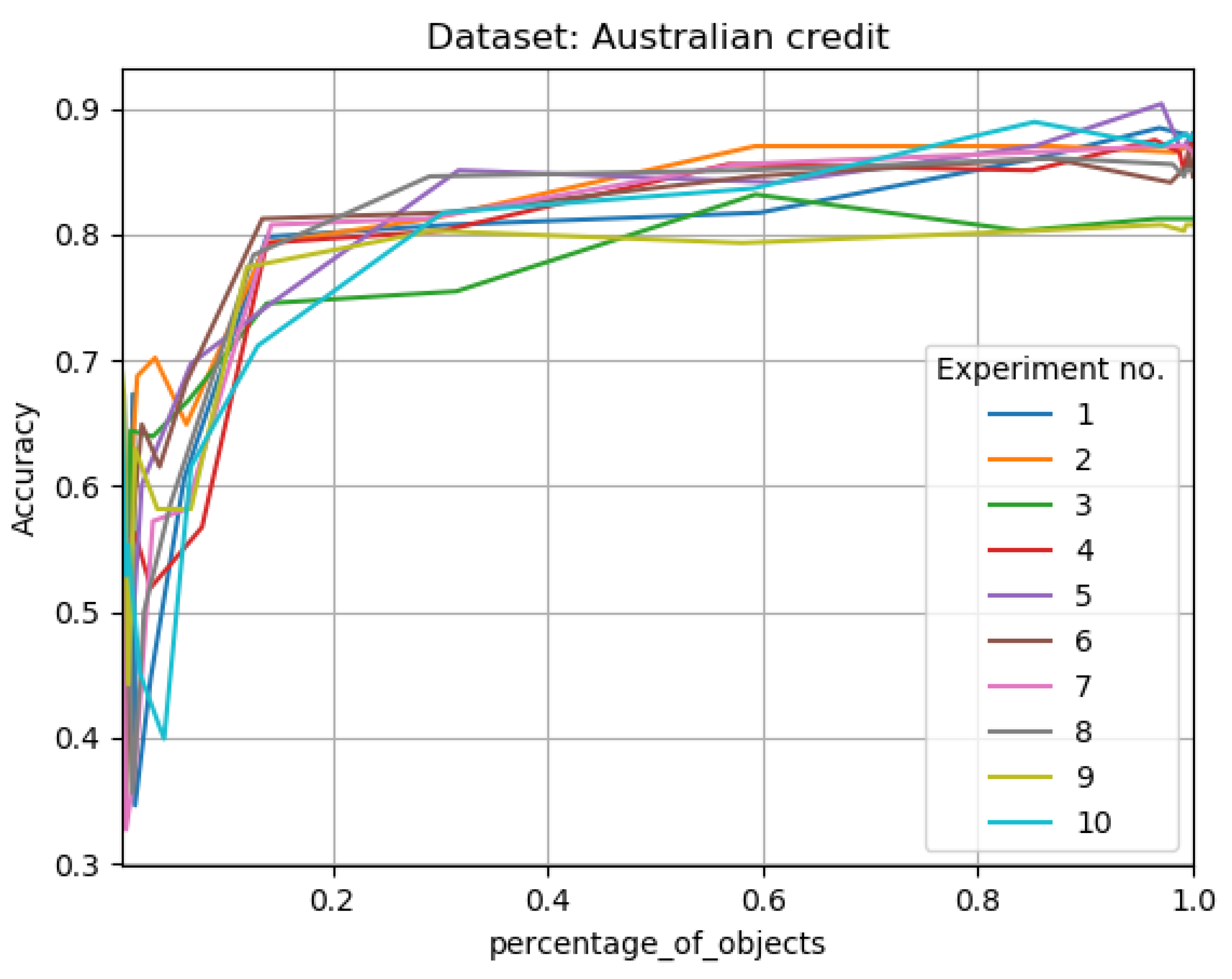
In the case of results for the Australian Credit system (see Figure 3 and Figure 4 and Table 5), within a radius of we get a reduction of about 70 percent and a classification accuracy of compared to 856 percent on the original system. In the case of radius, with a reduction of 41 per cent, we get an accuracy of . In case of radius , with reduction in training system size in the range od 14 percent, we have accuracy .
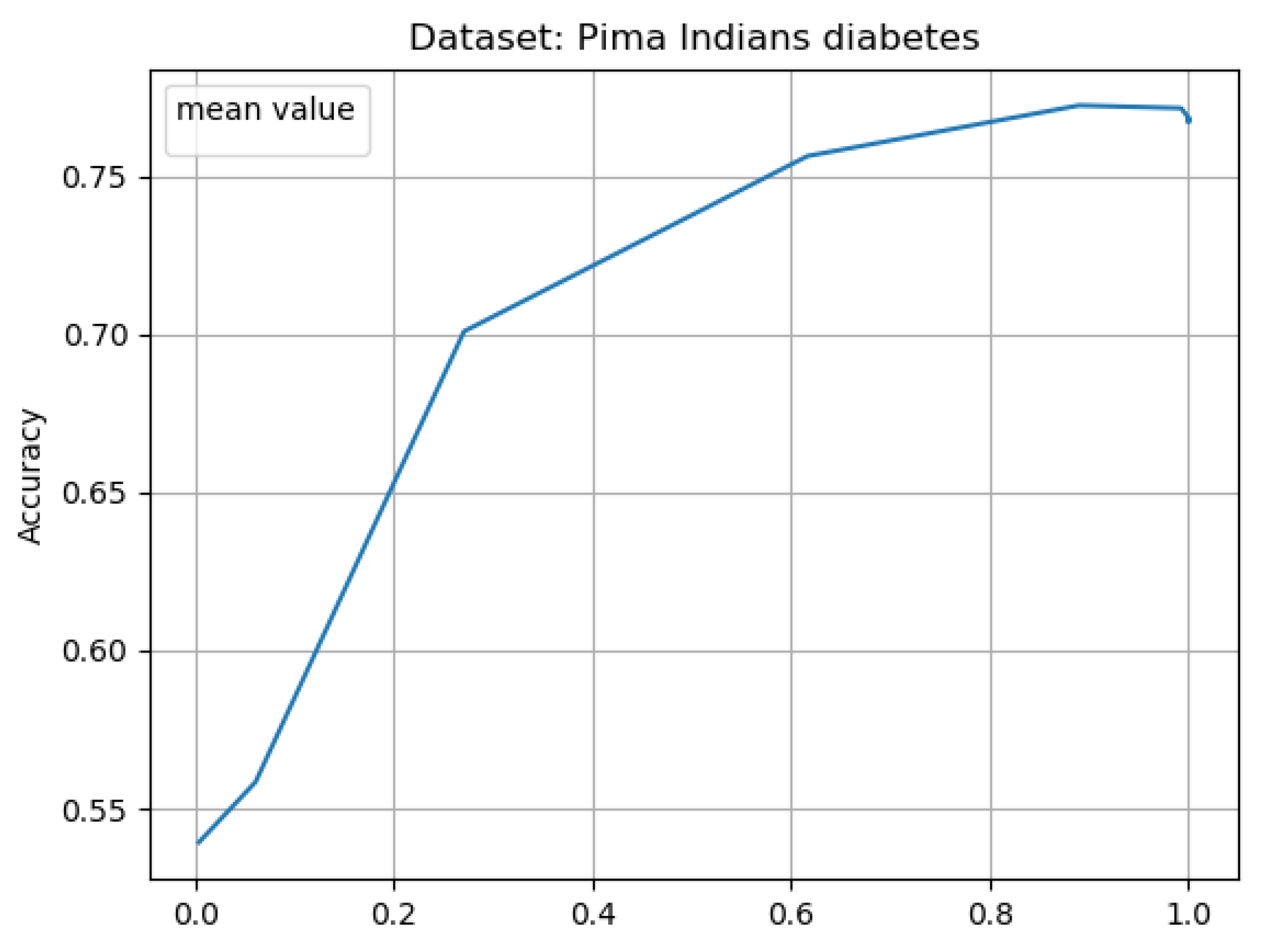
In our next experiment for the Pima Indians Diabetes system (see results in Figure 7 and Figure 8 and Table 7), for a radius of and a reduction in the number of objects of about 73 percent, we get an accuracy of compared to on non-granular data. In case of radius of and a reduction in the number of objects of about 38 percent, we get an accuracy of and finally for radius with 11 percent reduction we obtained accuracy .
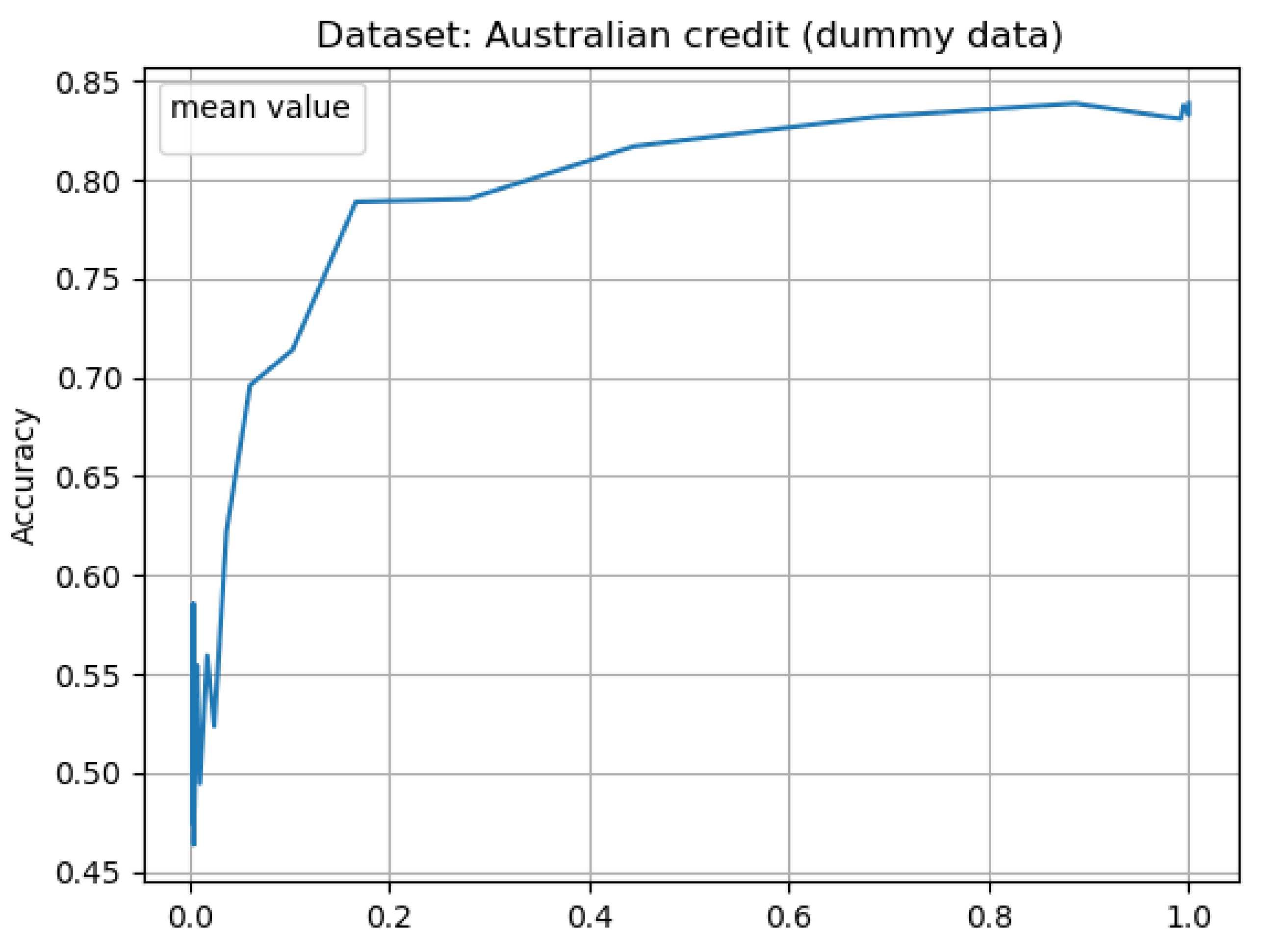
As an additional result, we added the learning effect of on the Australian credit data set after the conversion of its symbolic attributes to Dummy variables. From the results of Figure 9 and Figure 10 and Table 8 we see that the classification after the conversion is comparable. And exemplary result for radius , with 83 percent reduction in training set size, accuracy is equal . In case of radius , accuracy is with 55 percent reduction. For radius , with 31 percent reduction, we have reached accuracy . For radius equal with 11 percent reduction in training size, accuracy is . In the nil case for dummy variant accuracy is equal .
Despite the fact that the classification results are not the best among the techniques we have previously applied to granular data (among others Naive Bayes classifier [19]), SVM [21], Rough set based classifiers [19]), we are pleased that neural networks are able to maintain high classification efficiency by working on granular data. We treat the results as a trailer for future intensive research on the application of granular computing techniques in the context of learning neural networks.
The Table 5, Table 6, Table 7 and Table 8 present more information about our experiments. As an explanation please refer to the list of column labels and their explanation:
- gran_rad—granulation radius as a percentage value,
- no_of_gran_objects—number of new objects in tested decision system after the granulation process,
- percentage_of_objects—percentage of objects in tested decision system comparing to the primary decision system size,
- time_to_learn—time that was needed to complete the learning process using given data,
- accuracy—classification accuracy for given neural network.
5. Conclusions
This paper contains results that show how usage of granular reflections of decision systems can be used in deep learning. For experimental purpose we have selected the most effective method among the studied concept dependent variant and performed learning on selected data from the UCI Repository based on the tensorflow library. It turned out that the designed neural network works on approximated data in effective way, when measured in classification accuracy. Patterns contained in the granulated data seem to be preserved in the neural network structures. Experiments from our work have shown that our approximation techniques for tabular decision making systems can be an effective pre-processing step before learning with deep neural networks. Reduced data, while retaining internal knowledge, gives the opportunity for faster learning of networks. In future works we are planning to check the set of neural networks architectures to use with our approximation methods. We are considering the use of granular structures in the convolutionary part of the preparation of data for learning by means of neural networks.
Author Contributions
Conceptualization, K.R. and P.A.; Methodology, K.R. and P.A.; Software, K.R. and P.A.; Validation, K.R. and P.A.; Formal analysis, K.R. and P.A.; Investigation, K.R. and P.A.; Resources, K.R. and P.A.; Data curation, K.R. and P.A.; Writing—original draft preparation, K.R. and P.A.; Writing—review and editing, K.R. and P.A.; Visualization, K.R. and P.A.; Supervision, K.R. and P.A.; Project administration, K.R. and P.A.; Funding acquisition, K.R. and P.A. All authors have read and agreed to the published version of the manuscript.
Funding
This work has been fully supported by the grant from Ministry of Science and Higher Education of the Republic of Poland under the project number 23.610.007-000.
Conflicts of Interest
The authors declare no conflict of interest. The funders had no role in the design of the study; in the collection, analyses, or interpretation of data; in the writing of the manuscript, or in the decision to publish the results.
References
- Haykin, S.S. Neural Networks: A Comprehensive Foundation; Prentice Hall: Upper Saddle River, NJ, USA, 1999; ISBN 978-0-13-273350-2. [Google Scholar]
- Połap, D.; Woźniak, M.; Wei, W.; Damaševičius, R. Multi-threaded learning control mechanism for neural networks. Future Gener. Comput. Syst. 2018, 87, 16–34. [Google Scholar] [CrossRef]
- Woźniak, M.; Połap, D. Intelligent Home Systems for Ubiquitous User Support by Using Neural Networks and Rule-Based Approach. IEEE Trans. Ind. Inform. 2020, 16, 2651–2658. [Google Scholar] [CrossRef]
- Novikoff, A.B. On convergence proofs on perceptrons. In Proceedings of the Symposium on the Mathematical Theory of Automata, New York, NY, USA, 24–26 April 1962; Polytechnic Institute of Brooklyn: Brooklyn, NY, USA, 1962; Volume 12, pp. 615–622. [Google Scholar]
- Bryson, A.E.; Ho, Y.-C. Applied Optimal Control: Optimization, Estimation, and Control; Blaisdell Publishing Company: Waltham, MA, USA; Xerox College Publishing: Lexington, MA, USA, 1969; p. 481. [Google Scholar]
- Hochreiter, S.; Schmidhuber, J. Long short-term memory. Neural Comput. 1997, 9, 1735–1780. [Google Scholar] [CrossRef] [PubMed]
- Nielsen, M. Neural Networks and Deep Learning; Determination Press: San Francisco, CA, USA, 2015. [Google Scholar]
- Dick, S.; Kandel, A. Granular Computing in Neural Networks. In Granular Computing. Studies in Fuzziness and Soft Computing; Pedrycz, W., Ed.; Physica: Heidelberg, Germany, 2001; Volume 70. [Google Scholar]
- Leng, J.; Chen, Q.; Mao, N.; Jiang, P. Combining granular computing technique with deep learning for service planning under social manufacturing contexts. Knowl.-Based Syst. 2018, 143, 295–306, ISSN 0950-7051. [Google Scholar] [CrossRef]
- Ghiasi, B.; Sheikhian, H.; Zeynolabedin, A.; Niksokhan, M.H. Granular computing-neural network model for prediction of longitudinal dispersion coefficients in rivers. Water Sci. Technol. 2020. [Google Scholar] [CrossRef] [PubMed]
- Pawlak, Z. Rough Sets: Theoretical Aspects of Reasoning about Data; Kluwer: Alphen aan den Rijn, The Netherlands, 1991. [Google Scholar]
- Skowron, A.; Rauszer, C. The discernibility matrices and functions in information systems. In Intelligent Decision Support. Handbook of Applications and Advances of Rough Set Theory; Słowiński, R., Ed.; Kluwer Academic Publishers: Dordrecht, The Netherlands, 1992; pp. 331–362. [Google Scholar]
- Pawlak, Z.; Skowron, A. A rough set approach for decision rules generation. In Proceedings of the IJCAI’93 Workshop W12: The Management of Uncertainty in AI, Chambery Savoie, France, 30 August 1993; ICSResearch Report 23/93. Warsaw University of Technology: Warsaw, Poland, 1993. [Google Scholar]
- Polkowski, L.; Skowron, A. Rough mereology. In Proceedings of the ISMIS’94, Charlotte, NC, USA, 16–19 October 1994. LNCS 867. [Google Scholar]
- Polkowski, L. Approximate Reasoning by Parts. An Introduction to Rough Mereology; Springer: Berlin, Germany, 2011. [Google Scholar]
- Polkowski, L. A model of granular computing with applications. In Proceedings of the 2006 IEEE International Conference on Granular Computing, Atlanta, GA, USA, 10–12 May 2006. [Google Scholar]
- Polkowski, L. A unified approach to granulation of knowledge and granular computing based on rough mereology: A survey. In Handbook of Granular Computing; John Wiley and Sons: New York, NY, USA, 2008; pp. 375–401. [Google Scholar]
- Polkowski, L. Formal granular calculi based on rough inclusions. In Proceedings of the IEEE 2005 Conference on Granular Computing GrC05, Beijing, China, 25–27 July 2005; IEEE Press: New York, NY, USA; pp. 57–62. [Google Scholar]
- Polkowski, L.; Artiemjew, P. Granular Computing in Decision Approximation—An Application of Rough Mereology. In Intelligent Systems Reference Library 77; Springer: Berlin/Heidelberg, Germany, 2015; pp. 1–422. ISBN 978-3-319-12879-5. [Google Scholar]
- University of California. Irvine Machine Learning Repository. Available online: https://archive.ics.uci.edu/ml/index.php (accessed on 5 March 2020).
- Szypulski, J.; Artiemjew, P. The Rough Granular Approach to Classifier Synthesis by Means of SVM. In Proceedings of the International Joint Conference on Rough Sets, IJCRS’15, Tianjin, China, 20–23 November 2015; Lecture Notes in Computer Science (LNCS). Springer: Heidelberg, Germany, 2015; pp. 256–263. [Google Scholar]
Figure 1.
The diagram shows a scheme of our experimental part. The exact design of the neural network is in Figure 3. The data that is fed into the neural network is normalized after granulation to a range of .
Figure 1.
The diagram shows a scheme of our experimental part. The exact design of the neural network is in Figure 3. The data that is fed into the neural network is normalized after granulation to a range of .

Figure 2.
A diagram of the neural network used to learn the Australian credit system. Neural networks for the other two systems differ only in the number of inputs determined by the number of conditional attributes.
Figure 2.
A diagram of the neural network used to learn the Australian credit system. Neural networks for the other two systems differ only in the number of inputs determined by the number of conditional attributes.

Figure 3.
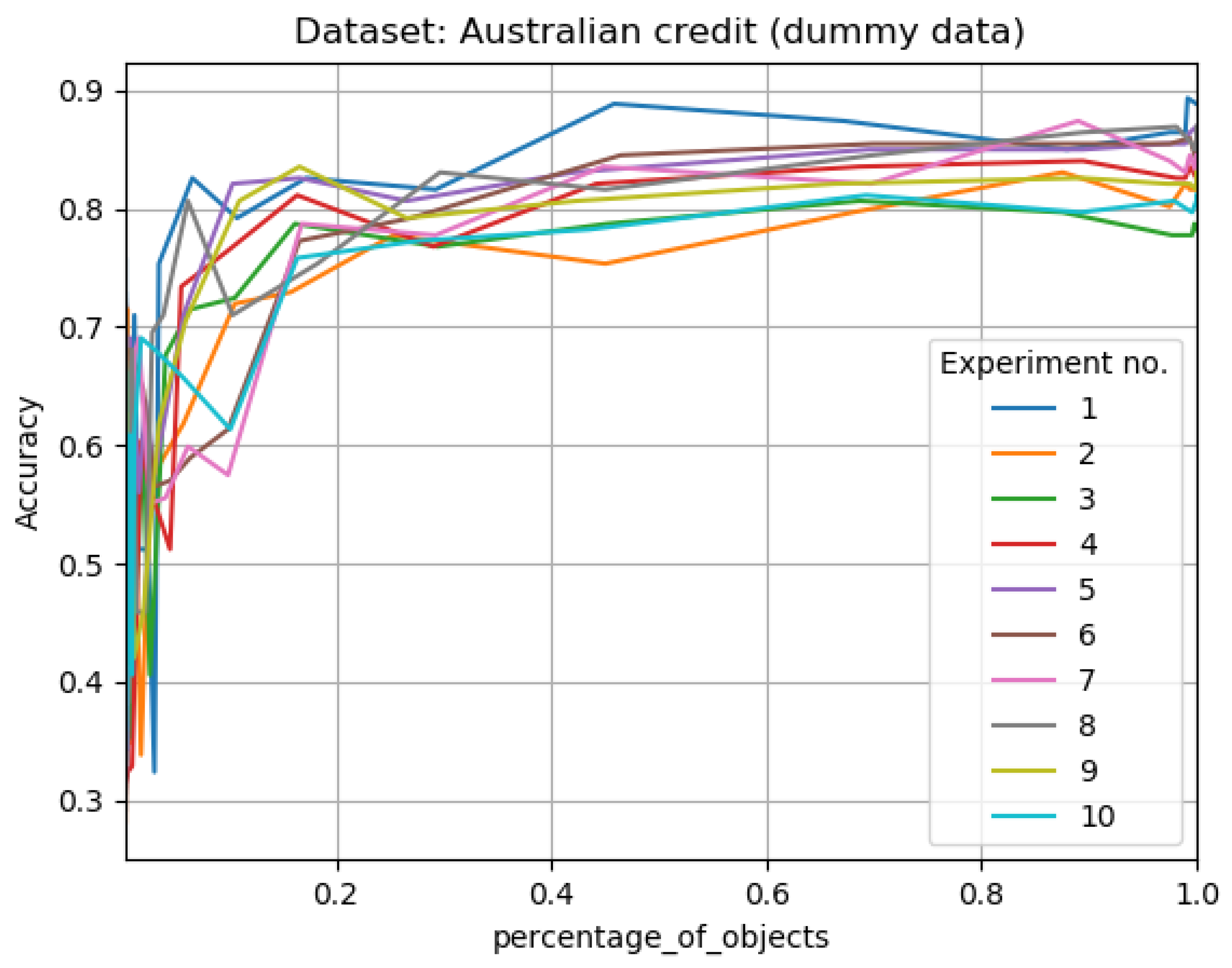
Results for 10 learning cycles, using 10 splits; for Australian credit data set; In ‘percentage of objects’ ax, we have the percentage size of granulated data vs accuracy of classification in ‘Accuracy’ ax; in. The results are not perfectly evenly matched or at the same points on the x-axis, due to the fact that the size reduction levels of the training systems varied.
Figure 3.
Results for 10 learning cycles, using 10 splits; for Australian credit data set; In ‘percentage of objects’ ax, we have the percentage size of granulated data vs accuracy of classification in ‘Accuracy’ ax; in. The results are not perfectly evenly matched or at the same points on the x-axis, due to the fact that the size reduction levels of the training systems varied.

Figure 4.
Mean result for 10 learning cycles, using 10 splits; for Australian credit data set; The only way to show the average values from the experiments was to calculate the average accuracy for specific granulation radii. Hence, on the x-axis we have the granulation radii (approximation levels). The figure shows the result from Table 5.

Figure 5.
Results for 10 learning cycles, using 10 splits; for Heart Disease data set; In ‘percentage of objects’ ax, we have the percentage size of granulated data vs accuracy of classification in ‘Accuracy’ ax; in. The results are not perfectly evenly matched or at the same points on the x-axis, due to the fact that the size reduction levels of the training systems varied.

Figure 6.
Mean result for 10 learning cycles, using 10 splits; for Heart disease data set; Mean result for 10 learning cycles, using 10 splits; for Australian credit data set; The only way to show the average values from the experiments was to calculate the average accuracy for specific granulation radii. Hence, on the x-axis we have the granulation radii (approximation levels). The figure shows the result from Table 6.

Figure 7.
Results for 10 learning cycles, using 10 splits; for Pima Indians Diabetes data set; In ‘percentage of objects’ ax, we have the percentege size of granulated data vs accuracy of classification in ‘Accuracy’ ax; in. The results are not perfectly evenly matched or at the same points on the x-axis, due to the fact that the size reduction levels of the training systems varied.

Figure 8.
Mean results for 10 learning cycles, using 10 splits; for Pima Indians Diabetes data set; Mean result for 10 learning cycles, using 10 splits; for Australian credit data set; The only way to show the average values from the experiments was to calculate the average accuracy for specific granulation radii. Hence, on the x-axis we have the granulation radii (approximation levels). The figure shows the result from Table 7.

Figure 9.
Results for 10 learning cycles, using 10 splits; for Australian credit data set converted to dummy variables (after conversion to dummy variables its 35 attributes); In ‘percentage of objects’ ax, we have the percentage size of granulated data vs accuracy of classification in ‘Accuracy’ ax; in. The results are not perfectly evenly matched or at the same points on the x-axis, due to the fact that the size reduction levels of the training systems varied.

Figure 10.
Dummy variables - mean result for 10 learning cycles, using 10 splits; for Australian credit data set; after conversion to Dummy variables its 35 attributes.
Figure 10.
Dummy variables - mean result for 10 learning cycles, using 10 splits; for Australian credit data set; after conversion to Dummy variables its 35 attributes.


Table 1.
The training decision system .
| d | |||||
|---|---|---|---|---|---|
| 2 | 1 | 2 | 1 | 1 | |
| 3 | 2 | 3 | 3 | 1 | |
| 1 | 5 | 1 | 2 | 1 | |
| 6 | 2 | 3 | 8 | 2 | |
| 4 | 5 | 8 | 6 | 2 | |
| 5 | 1 | 8 | 1 | 2 |
Table 2.
gcdm (
| 1 | 0 | 0 | x | x | x | |
| 0 | 1 | 0 | x | x | x | |
| 0 | 0 | 1 | x | x | x | |
| x | x | x | 1 | 0 | 0 | |
| x | x | x | 0 | 1 | 1 | |
| x | x | x | 0 | 1 | 1 |
Table 3.
Concept dependent granular decision system for and radius 0.25.
| 2 | 1 | 2 | 1 | 1 | |
| 3 | 2 | 3 | 3 | 1 | |
| 1 | 5 | 1 | 2 | 1 | |
| 6 | 2 | 3 | 8 | 2 | |
| 5 | 5 | 8 | 6 | 2 |
Table 4.
Exemplary decision systems from UCI Machine Learning Repository [20]. We have chosen binary systems.
Table 4.
Exemplary decision systems from UCI Machine Learning Repository [20]. We have chosen binary systems.
| 15 | 690 | |
| 9 | 768 | |
| 14 | 270 |
Table 5.
Results for Australian credit dataset (mean from 10 experiments).
| no_of_gran_objects | percentage_of_objects | time_to_learn | accuracy | |
|---|---|---|---|---|
| Mean | Mean | Mean | Mean | |
| gran_rad | ||||
| 0.0667 | 2.0 | 0.4149 | 0.3666 | 0.5646 |
| 0.1333 | 2.0 | 0.4149 | 0.3607 | 0.5337 |
| 0.2000 | 3.4 | 0.7054 | 0.3691 | 0.5423 |
| 0.2667 | 5.1 | 1.0581 | 0.3685 | 0.5154 |
| 0.3333 | 8.2 | 1.7012 | 0.3696 | 0.5192 |
| 0.4000 | 16.0 | 3.3195 | 0.3778 | 0.5577 |
| 0.4667 | 31.6 | 6.5560 | 0.3777 | 0.6236 |
| 0.5333 | 65.3 | 13.5477 | 0.3916 | 0.7764 |
| 0.6000 | 145.3 | 30.1452 | 0.4287 | 0.8125 |
| 0.6667 | 283.8 | 58.8797 | 0.7464 | 0.8399 |
| 0.7333 | 412.9 | 85.6639 | 0.8210 | 0.8534 |
| 0.8000 | 468.8 | 97.2614 | 0.8585 | 0.8587 |
| 0.8667 | 477.9 | 99.1494 | 0.8532 | 0.8553 |
| 0.9333 | 479.3 | 99.4398 | 0.8817 | 0.8553 |
| 1.0000 | 482.0 | 100.0000 | 0.8995 | 0.8562 |
Table 6.
Results for Heart disease dataset (mean from 10 experiments).
| no_of_gran_objects | percentage_of_objects | time_to_learn | accuracy | |
|---|---|---|---|---|
| Mean | Mean | Mean | Mean | |
| gran_rad | ||||
| 0.0714 | 2.0 | 0.9434 | 0.3702 | 0.6801 |
| 0.1429 | 2.3 | 1.0849 | 0.3786 | 0.6505 |
| 0.2143 | 2.8 | 1.3208 | 0.3708 | 0.6231 |
| 0.2857 | 4.5 | 2.1226 | 0.3758 | 0.7132 |
| 0.3571 | 8.8 | 4.1509 | 0.3928 | 0.7110 |
| 0.4286 | 17.0 | 8.0189 | 0.4064 | 0.7187 |
| 0.5000 | 35.7 | 16.8396 | 0.4209 | 0.7198 |
| 0.5714 | 70.4 | 33.2075 | 0.4299 | 0.7560 |
| 0.6429 | 122.7 | 57.8774 | 0.4571 | 0.7813 |
| 0.7143 | 177.9 | 83.9151 | 0.4872 | 0.8231 |
| 0.7857 | 204.6 | 96.5094 | 0.4942 | 0.8297 |
| 0.8571 | 211.4 | 99.7170 | 0.4995 | 0.8220 |
| 0.9286 | 211.4 | 99.7170 | 0.5023 | 0.8209 |
| 1.0000 | 211.4 | 99.7170 | 0.5010 | 0.8253 |
Table 7.
Results for Pima Indians Diabetes dataset (mean from 10 experiments).
| no_of_gran_objects | percentage_of_objects | time_to_learn | accuracy | |
|---|---|---|---|---|
| Mean | Mean | Mean | Mean | |
| gran_rad | ||||
| 0.1111 | 2.0 | 0.3724 | 0.3679 | 0.5392 |
| 0.2222 | 32.6 | 6.0708 | 0.4544 | 0.5584 |
| 0.3333 | 145.3 | 27.0577 | 0.4899 | 0.7009 |
| 0.4444 | 331.0 | 61.6387 | 0.7895 | 0.7563 |
| 0.5556 | 477.8 | 88.9758 | 0.8457 | 0.7723 |
| 0.6667 | 533.0 | 99.2551 | 0.8643 | 0.7714 |
| 0.7778 | 537.0 | 100.0000 | 0.8882 | 0.7684 |
| 0.8889 | 537.0 | 100.0000 | 0.9313 | 0.7671 |
| 1.0000 | 537.0 | 100.0000 | 0.9417 | 0.7680 |
Table 8.
Dummy variables—results for Australian credit dataset (mean from 10 experiments; after conversion to Dummy variables its 35 attributes).
Table 8.
Dummy variables—results for Australian credit dataset (mean from 10 experiments; after conversion to Dummy variables its 35 attributes).
| no_of_gran_objects | percentage_of_objects | time_to_learn | accuracy | |
|---|---|---|---|---|
| Mean | Mean | Mean | Mean | |
| gran_rad | ||||
| 0.025 | 2.0 | 0.4149 | 0.3598 | 0.5534 |
| 0.050 | 2.0 | 0.4149 | 0.4274 | 0.5647 |
| 0.075 | 2.0 | 0.4149 | 0.4314 | 0.4836 |
| 0.100 | 2.0 | 0.4149 | 0.4373 | 0.4744 |
| 0.125 | 2.0 | 0.4149 | 0.4391 | 0.5536 |
| 0.150 | 2.0 | 0.4149 | 0.4327 | 0.5841 |
| 0.175 | 2.0 | 0.4149 | 0.4305 | 0.5778 |
| 0.200 | 2.0 | 0.4149 | 0.4349 | 0.4928 |
| 0.225 | 2.0 | 0.4149 | 0.4404 | 0.4826 |
| 0.250 | 2.0 | 0.4149 | 0.4348 | 0.5048 |
| 0.275 | 2.0 | 0.4149 | 0.4342 | 0.5082 |
| 0.300 | 2.0 | 0.4149 | 0.4586 | 0.5261 |
| 0.325 | 2.0 | 0.4149 | 0.4494 | 0.5652 |
| 0.350 | 2.0 | 0.4149 | 0.4476 | 0.5130 |
| 0.375 | 2.0 | 0.4149 | 0.4369 | 0.4797 |
| 0.400 | 2.0 | 0.4149 | 0.4608 | 0.5329 |
| 0.425 | 2.0 | 0.4149 | 0.4444 | 0.5256 |
| 0.450 | 2.0 | 0.4149 | 0.4443 | 0.5179 |
| 0.475 | 2.0 | 0.4149 | 0.4516 | 0.5135 |
| 0.500 | 2.0 | 0.4149 | 0.4436 | 0.5855 |
| 0.525 | 2.0 | 0.4149 | 0.4417 | 0.5034 |
| 0.550 | 2.2 | 0.4564 | 0.4517 | 0.4638 |
| 0.575 | 2.9 | 0.6017 | 0.4431 | 0.5063 |
| 0.600 | 3.7 | 0.7676 | 0.4476 | 0.5546 |
| 0.625 | 5.2 | 1.0788 | 0.4571 | 0.4947 |
| 0.650 | 8.7 | 1.8050 | 0.4506 | 0.5594 |
| 0.675 | 12.1 | 2.5104 | 0.4754 | 0.5237 |
| 0.700 | 18.0 | 3.7344 | 0.4782 | 0.6222 |
| 0.725 | 29.4 | 6.0996 | 0.5029 | 0.6961 |
| 0.750 | 49.9 | 10.3527 | 0.5087 | 0.7140 |
| 0.775 | 80.4 | 16.6805 | 0.5228 | 0.7889 |
| 0.800 | 134.8 | 27.9668 | 0.7577 | 0.7903 |
| 0.825 | 214.3 | 44.4606 | 0.8252 | 0.8169 |
| 0.850 | 331.3 | 68.7344 | 0.8719 | 0.8319 |
| 0.875 | 427.3 | 88.6515 | 0.9257 | 0.8386 |
| 0.900 | 470.7 | 97.6556 | 0.9505 | 0.8319 |
| 0.925 | 478.2 | 99.2116 | 0.9665 | 0.8309 |
| 0.950 | 479.5 | 99.4813 | 0.9729 | 0.8377 |
| 0.975 | 482.0 | 100.0000 | 0.9688 | 0.8329 |
| 1.000 | 482.0 | 100.0000 | 0.9697 | 0.8386 |
© 2020 by the authors. Licensee MDPI, Basel, Switzerland. This article is an open access article distributed under the terms and conditions of the Creative Commons Attribution (CC BY) license (http://creativecommons.org/licenses/by/4.0/).
Share and Cite
MDPI and ACS Style
Ropiak, K.; Artiemjew, P. On a Hybridization of Deep Learning and Rough Set Based Granular Computing. Algorithms 2020, 13, 63. https://0-doi-org.brum.beds.ac.uk/10.3390/a13030063
AMA Style
Ropiak K, Artiemjew P. On a Hybridization of Deep Learning and Rough Set Based Granular Computing. Algorithms. 2020; 13(3):63. https://0-doi-org.brum.beds.ac.uk/10.3390/a13030063
Chicago/Turabian StyleRopiak, Krzysztof, and Piotr Artiemjew. 2020. "On a Hybridization of Deep Learning and Rough Set Based Granular Computing" Algorithms 13, no. 3: 63. https://0-doi-org.brum.beds.ac.uk/10.3390/a13030063
Note that from the first issue of 2016, this journal uses article numbers instead of page numbers. See further details here.