Experiments-Based Comparison of Different Power Controllers for a Solid Oxide Fuel Cell Against Model Imperfections and Delay Phenomena

Abstract

Solid oxide fuel cell systems such as those presented in this paper are not only applicable for a pure supply with electric energy, they can typically also be used in decentralized power stations, i.e., as micro-cogeneration systems for houses, where both electric and thermal energy are required. For that application, obviously, the electric power need is not constant but rather changes over time. In such a way, it essentially depends on the user profiles of said houses which can refer to e.g., private households as well as offices. The power use is furthermore not predefined. For an optimal operation of the fuel cell, we want to adjust the power, to match the need with sufficiently small time constants without the implementation of mid- or long-term electrical storage systems such as battery buffers. To adapt the produced electric power a simple, however, sufficiently robust feedback controller regulating the hydrogen mass flow into the cells is necessary. To achieve this goal, four different controllers, namely, a PI output-feedback controller combined with a feedforward control, an internal model control (IMC) approach, a sliding-mode (SM) controller and a state-feedback controller, are developed and compared in this paper. As the challenge is to find a controller ensuring steady-state accuracy and good tracking behavior despite the nonlinearities and uncertainties of the plant, the comparison was done regarding these requirements. Simulations and experiments show that the IMC outperforms the alternatives with respect to steady-state accuracy and tracking behavior.

1. Introduction

Especially in the wake of climate change and the resulting rethink in energy production, renewed attention has directed itself towards fuel cells. The progressing research in the area of solid oxide fuel cells (SOFCs) [1,2,3] creates a lot of novel applications, e.g., stationary installed, decentralized micro-cogeneration systems for houses providing both heat and electricity. Regarding the power need for different types of houses, it becomes clear that it varies depending on each house individually not only in the absolute power demand but also with respect to its temporal—daily and seasonal—profile. Because we want to include private households as well as industrial users such as offices, which are obviously characterized by significantly different daily, weekly, and seasonal characteristics regarding the times and variability of high energy needs, a dynamic operation strategy based on the current power demand should be implemented to take into account all possible usages of these micro-cogeneration systems.

In an SOFC, the electric current and power production occurs due to internal cold combustion. Providing optimal conditions for this combustion is the long-term goal for a useful operation. Although the electric power maximum of an SOFC is typically specified by adaptations of the electric stack current (partially on the basis of real-time capable parameter identification and optimization procedures such as those recently published by Rauh et al., cf. [4]), short-term adjustments of the produced electric power can effectively by realized by variations of the inlet hydrogen mass flow at the anode side. Note that the prespecification of the average operating point, defined by a triplet of hydrogen mass flow, electric stack current, and resulting electric power, has to be performed in such a way as to guarantee safe and wearless operation. This is given by making sure that the average operating point lies within the region of the current–power characteristic that has a positive slope. Overshooting its maximum should be avoided, for example by means of the techniques presented in [4]. Therefore, the control strategies presented in this paper aim at realizing power adaptations by means of the hydrogen mass flow as control input in the neighborhood of suitable operating points that fully lie within the domain of Ohmic polarization [5]. Hence, the measure of adapting the hydrogen mass flow, to meet the consumers’ need as long as the fuel cell stack is operated in part-load conditions. To achieve this type of electric power control, four different approaches are introduced in this paper. Here, at first, a basic PI controller in combination with a feedforward control was implemented, followed by an internal model controller, a sliding-mode controller, and a linear state-feedback controller. Concerning robustness against imperfectly known gains and time constants of the plant, all of them were compared to each other in a simulation. This numerical evaluation was performed with respect to the controllers’ behavior in terms of best steady-state accuracy in combination with a good reference tracking behavior.

State-of-the-art approaches for electric power control of solid oxide fuel cells, which are based on manipulating the anode gas mass flow, can be subdivided into two different categories: Firstly, offline generated look-up tables relating the electric power of a fuel cell stack to its inlet gas mass flow and electric current are applicable to implement quasi-static open-loop control approaches. Although the offline generation of such look-up tables requires a time-consuming, stack-specific experimental identification, such static mappings become inaccurate as soon as the stack temperature, the inlet gas temperatures, and the composition of the supplied gases, which is especially relevant for the use of external gas reformers, deviate from the conditions present during the identification phase. To circumvent such phenomena, feedback controllers are typically employed. However, the use of dynamic models, taking into account a sufficiently large number of physical as well as electrochemical processes (such as variations of gas partial pressures and the diffusion-driven exchange of charge carriers in the cell membranes) are typically too complex to allow for a real-time capable control implementation. Therefore, this paper does not aim at using a model-based predictive control technique, based on a physically motivated detailed dynamics representation such as used in [6] for polymer electrolyte fuel cells, which could from a methodological point of view be transferred analogously to the case of SOFCs. Existing alternatives, such as nominal quasi-static relations for the relation between the supplied gas mass flows and the resulting electric power given in [7,8] tackle the issue of a time consuming look-up table generation. However, they still become inaccurate if at least one of the reasons for deviations mentioned above occur. Therefore, to keep the control technique as simple as possible, and to make it readily applicable in an industrial context, we purposefully decided to perform a control synthesis on an experimentally identified linear approximation of the input–output behavior of the electrochemical subsystem of the SOFC. Future work will allow combining our experimentally identified transfer function models with the representations given in [7,8] so that the domains in which the controllers work accurately in a robust manner can be extended.

The aforementioned experimentally identified system model is given in terms of a finite-order, linear time-invariant transfer function, which captures the following effects:

• lag behavior of the gas supply valves;
• gas transport phenomena in gas supply tubes in combination with the delayed power variation if the amount of supplied fuel is changed; and
• the stationary gain between a constant gas supply and the resulting electric power for a representative current with approximately constant thermal operating conditions.

It is, however, obvious that a linear time-invariant model cannot account for temporal (or state-dependent) coefficient changes. It has to be noted that the neglected phenomena act virtually on the linear plant model such as additive input disturbances. Hence, an integral output error feedback, IMC strategies as well as sliding-mode approaches that are capable of counteracting matched input disturbances are especially promising to implement a robust controller according to the aforementioned design aims.

All controllers considered in this paper are, hence, developed on the basis of the experimentally identified input–output behavior of the electrochemical subsystem of the SOFC. This input–output behavior was determined by the Matlab transfer function estimator [9] using the experimental data gathered during previous work [10,11,12]. Details about this experiments-based modeling are presented in Section 2. For the controller design in Section 3, the a priori identified system was approximated by transfer functions of different order with delay representations that are given in terms of rational, minimum-phase transfer function elements. In addition, mass flow lag dynamics of the supply caused by the actuators inside the plant of the SOFC system were accounted for. Each controller was analyzed regarding its robustness against measurement noise and uncertainties in the plant dynamics including a gain mismatch of several tens of percent, as shown in Section 4. The two best controllers of this simulation case study, namely, the PI controller and the IMC, were implemented at a test rig available at the Chair of Mechatronics, University of Rostock to validate the results of the simulation in Section 5. Finally, Section 6 gives a conclusion and some insight on future work.

2. Modeling the Electrochemical Behavior

In an SOFC, both electric and thermal energy are produced simultaneously by the cold combustion. However, the overall SOFC process can be split into its thermal and electrochemical behavior for the mathematical description. Since the aim in the presented paper is to design an electric power controller, we restrict ourselves to the electrochemical behavior. All other phenomena, such as the inevitable variation of the stack temperature caused by exothermal reaction enthalpies which are not fully suppressed by adjustments of the cathode gas inlet temperature [10,12,13,14,15], are treated as non-modeled disturbances from the point of view of the electrochemical subsystem.

In general, the electric current of a fuel cell is a result of the redox-reaction [16]

$$\begin{array}{cc}2{\mathrm{H}}_2+2{\mathrm{O}}^{2-}\to 2{\mathrm{H}}_2\mathrm{O}+4e^{-}& \hfill (\mathrm{oxidation}\mathrm{at}\mathrm{the}\mathrm{anode})\\ {\mathrm{O}}_2+4e^{-}\to 2{\mathrm{O}}^{2-}& \hfill (\mathrm{reduction}\mathrm{at}\mathrm{the}\mathrm{cathode})\\ 2{\mathrm{H}}_2\left(g\right)+{\mathrm{O}}_2\left(g\right)\to 2{\mathrm{H}}_2\mathrm{O}\left(g\right)& \hfill (\mathrm{redox}-\mathrm{reaction}).\end{array}$$

(1)

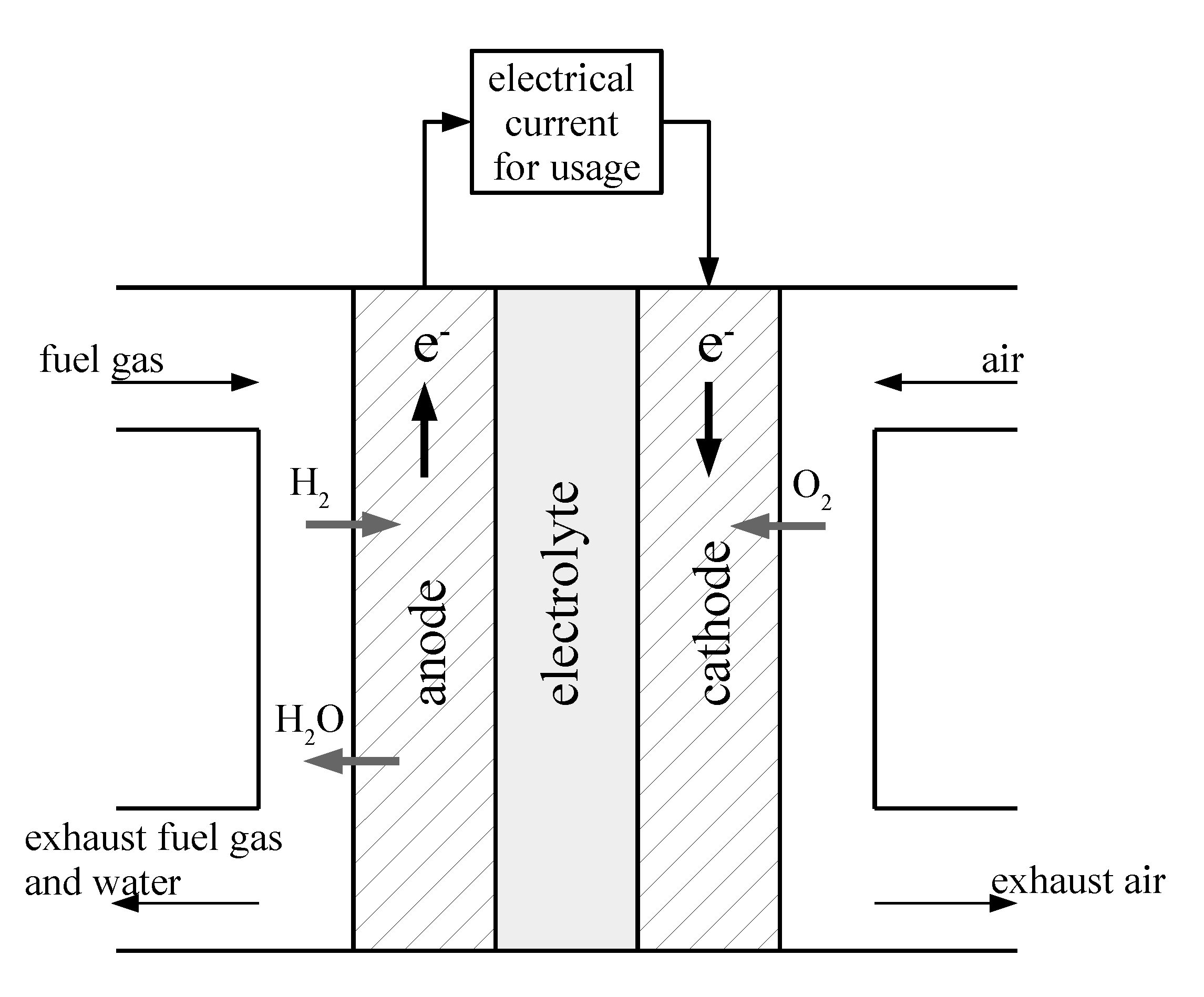
As shown in Figure 1, the supplied hydrogen gas reacts with oxygen ions at the anode. Free electrons flow through an external circuit, which is implemented at the available test rig as a variable Ohmic resistor. In such a way, the fuel cell, respectively, the series concatenation of multiple cells in a corresponding stack module, serves as a directed current source for the consumer. Finally, the produced flow of electrons reaches the cathode to react with oxygen that is supplied in terms of preheated ambient air.

The resulting instantaneous power, which can be calculated from the measured current and voltage at the SOFC’s terminals should be controlled, which is the aim of this paper under the assumption that the electric current is kept constant by the controllable load resistor. In previous work (cf. [10,11,12]), some experiments were performed to solve modeling problems especially related to the control-oriented characterization of the thermal fuel cell behavior in various operating points. Based on these measured data, the linear time-invariant transfer function of the SOFC system

$$\begin{array}{cc}{G}_{\mathrm{S}}\left(s\right)\hfill & ={\displaystyle \frac{P_{\mathrm{el}}\left(s\right)}{{\dot{m}}_{{\mathrm{H}}_2}\left(s\right)}}\hfill \\ & ={\displaystyle \frac{2.903\times {10}^5{s}^5+5.189\times {10}^4{s}^4+7.504\times {10}^3{s}^3+8.643\times {10}^2{s}^2+2.908\times {10}^{1}s+3.262\times {10}^{-1}}{s^6+8.229\times {10}^{-2}{s}^5+2.018\times {10}^{-2}{s}^4+8.309\times {10}^{-4}{s}^3+9.233\times {10}^{-5}{s}^2+1.558\times {10}^{-6}s+1.033\times {10}^{-8}}}\hfill \end{array}$$

(2)

was determined with the help of the Matlab transfer function estimator [9], to describe the correlation between the electric power $P_{\mathrm{el}}$ as the measured output and the hydrogen mass flow ${\displaystyle {\dot{m}}_{{\mathrm{H}}_2}}$ as the input under the aforementioned assumption of a constant electric current and a reliable temperature control keeping the average stack temperature in the close vicinity of the operating point that is equally used for identification and control purposes.

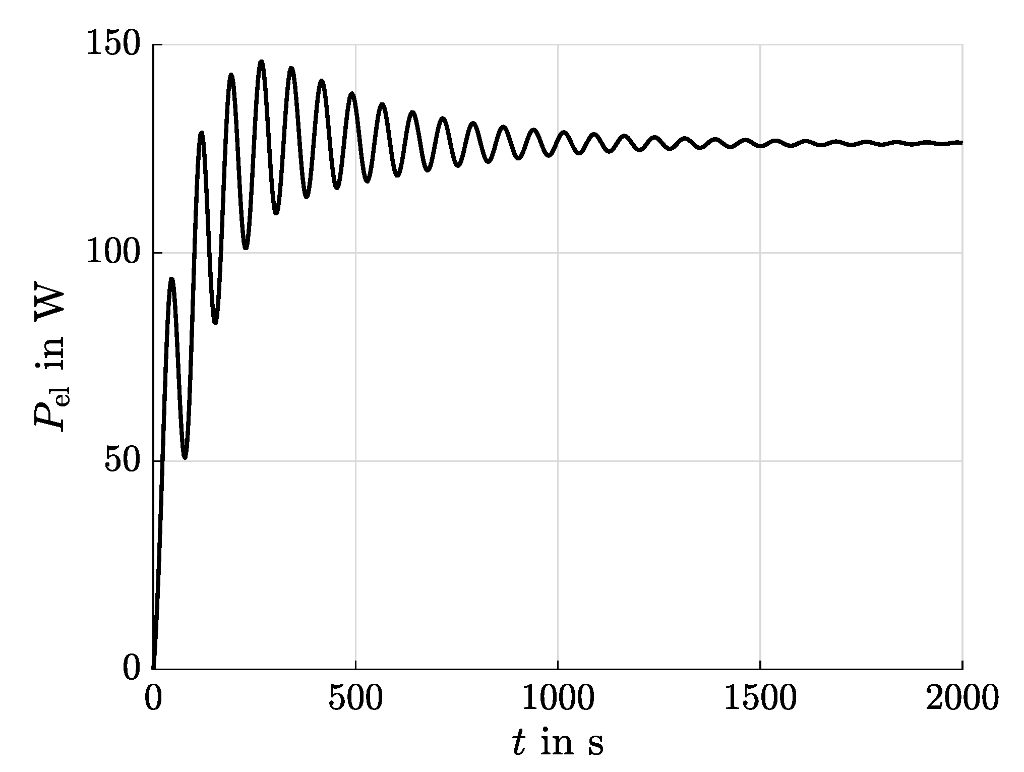
Remark 1.

Oscillations in the depicted step response in Figure 2 are mostly related to long gas supply tubes and the fluidic inertia of the anode gas mass flow between the control value and the SOFC stack. For visualization purposes, ${\dot{m}}_{{\mathrm{H}}_2}=4\times {10}^{-6}\frac{\mathrm{kg}}{\mathrm{s}}$ has been used.

3. Controller Design

For the controller design, a simplified representation of the approximated SOFC system in Equation (2)

$$G_{\mathrm{S},\mathrm{PT}i}={\displaystyle \frac{b}{{\sum }_{\nu =i-1}^n{a}_{\nu }·s^{\nu }}}\mathrm{with}i\in \{1,\dots ,n\},a_n=1$$

(3)

is used. Here, different choices for the order n are made for each controller in the following subsections.

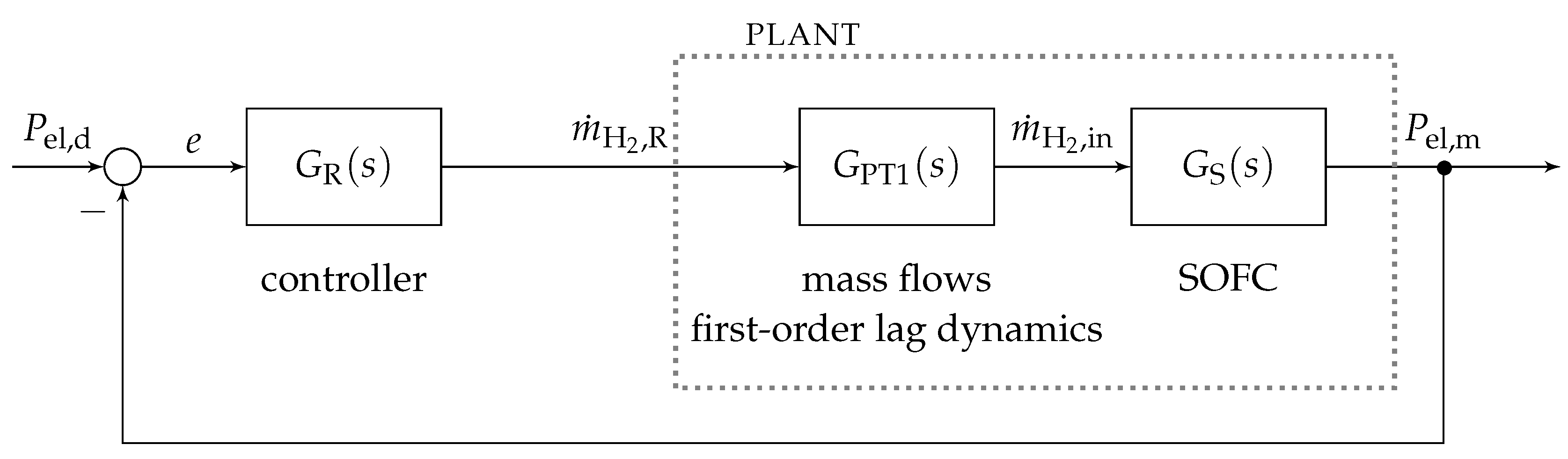
Since we do not know the actual power need commanded by the SOFC user, the controller should follow a smooth trajectory comprising phases of both increasing and decreasing electric power with good tracking accuracy. For this, four controllers, three linear and one nonlinear, were developed and compared with each other. 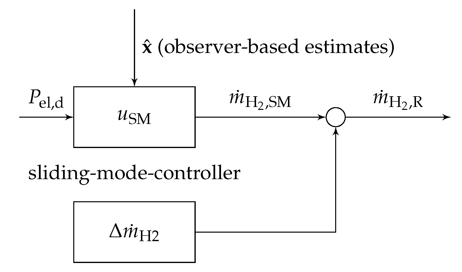Assuming that a potential consumer specifies the desired power $P_{\mathrm{el}},\mathrm{d}$, the reference variable is given and the difference to the measured power $P_{\mathrm{el}},\mathrm{m}$ can be made use of, as shown in Figure 3. The controller determines the hydrogen gas mass flow ${\dot{m}}_{{\mathrm{H}}_2},\mathrm{R}$ as the manipulated input variable into the plant.

In addition to the transfer function in Equation (2), the hydrogen gas mass flow ${\dot{m}}_{{\mathrm{H}}_2}$, representing the stack inlet ${\dot{m}}_{{\mathrm{H}}_2,\mathrm{in}}$ from the previous section, has a significantly delayed reaction to the commanded signal ${\dot{m}}_{{\mathrm{H}}_2,\mathrm{R}}$ of the manipulated input variable. This is considered in the additional transfer function

$$G_{\mathrm{PT}1}\left(s\right)={\displaystyle \frac{{\dot{m}}_{{\mathrm{H}}_2,\mathrm{in}}\left(s\right)}{{\dot{m}}_{{\mathrm{H}}_2,\mathrm{R}}\left(s\right)}}={\displaystyle \frac{1}{20s+1}},$$

(4)

with a time constant of 20 s, which was also determined based on measured data. This first-order lag element is taken into account in the design of each of the following control laws.

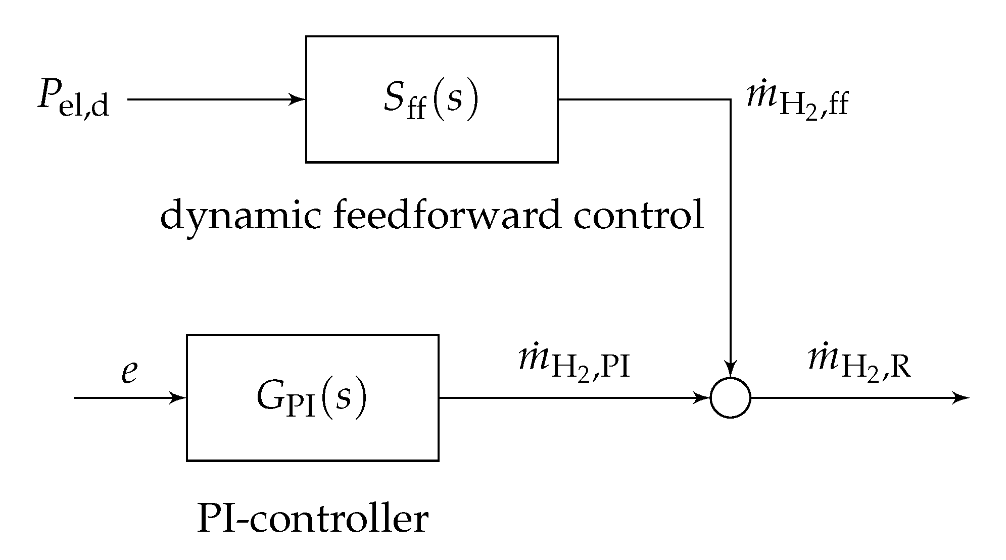
3.1. PI Control with Feedforward Control

First, the power control is realized with a PI controller according to the transfer function

$$G_{\mathrm{PI}}\left(s\right)=K_{\mathrm{R}}·{\displaystyle \frac{T_{\mathrm{I}}·s+1}{T_{\mathrm{I}}·s}}$$

(5)

combined with a simplified dynamic feedforward control, as shown in Figure 4.

Usually, the integral term in the PI controller already leads to robustness against static gain errors [17]. However, it needs to be chosen in such a way that a compromise is found between damping and fast transient responses, because of the influence of the parameter $T_{\mathrm{I}}$ on the overall phase reserve. Basically, it is set equal to the largest plant time constant of Equation (2). For the simplified dynamic feedforward control design, the SOFC system is approximated by

$$G_{\mathrm{S},\mathrm{PT}1}\left(s\right)={\displaystyle \frac{4.119\times {10}^5}{s+1.279\times {10}^{-2}}}$$

(6)

resulting in

$$S_{\mathrm{ff}}\left(s\right)=G_{\mathrm{S},\mathrm{PT}1}{\left(s\right)}^{-1}$$

(7)

as the dynamic feedforward control.

Remark 2.

The gain $K_{\mathrm{R}}$ needs to be kept small enough so that actuator saturations are not reached which may provoke undesirable integrator wind-up phenomena.

Remark 3.

As shown in both simulations and experiments, the PI controller has the drawback in the case of non-modeled nonlinearities and deviations between the plant and the design model, in which a compensation for this mismatch can only take place by the integral control action after a sufficiently large tracking error has occurred.

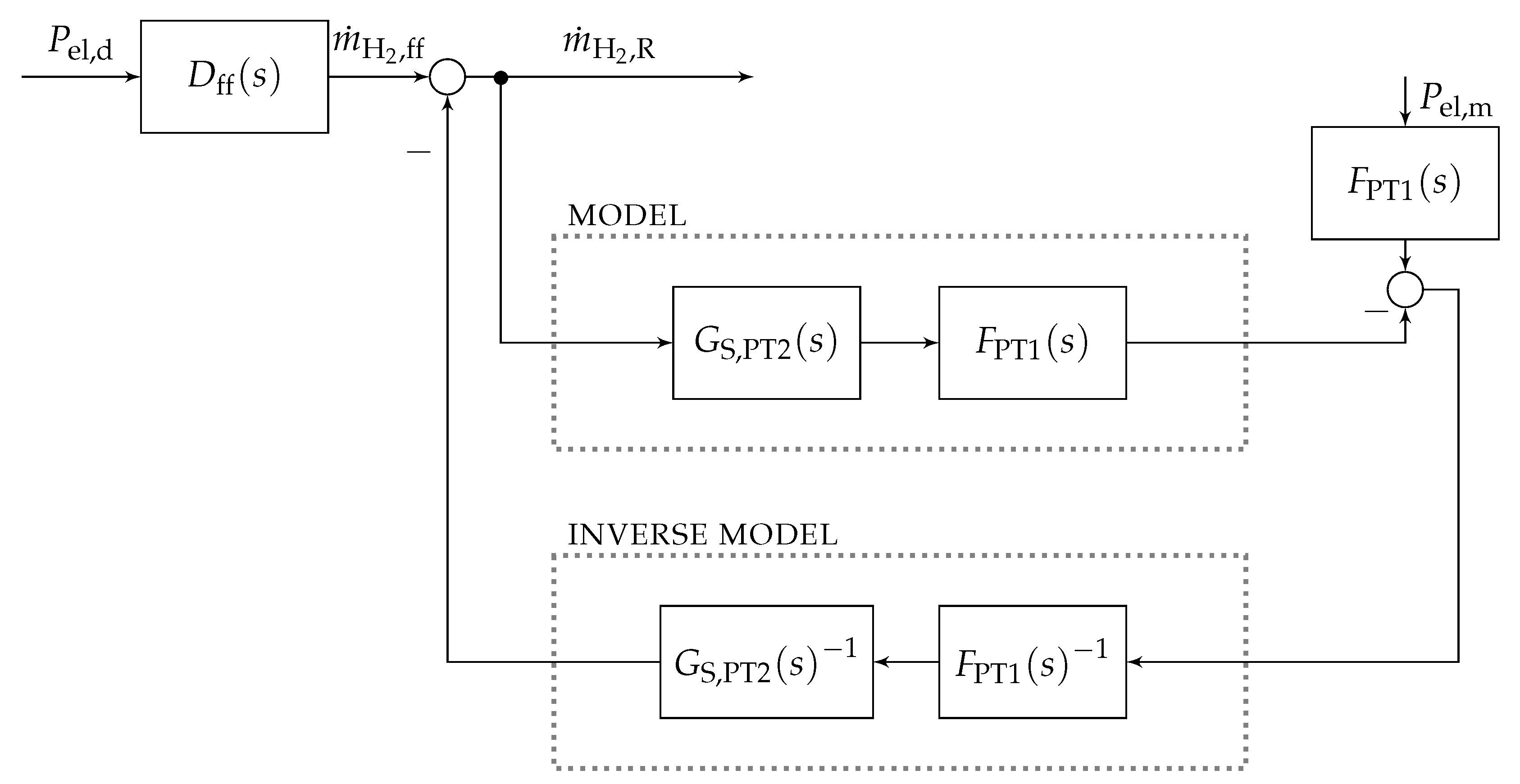
3.2. Internal Model Control

The internal model control (IMC) is a model-based methodology for controller design comprising the controller itself and a model of the real process. In contrast to other controllers, the feedback signal consists of the difference between the real process and its mathematical model instead of measured or estimated states. This special structure, shown in Figure 5, allows for inherent robustness against model uncertainties [18] by forcing the true system dynamics to behave similar to the transfer function included in the parallel model path. Deviations caused by additive input disturbances are usually compensated with high accuracy as long as the plant model is sufficiently close to reality.

Here, the model of the SOFC system is approximated by the second-order dynamics

$$G_{\mathrm{S},\mathrm{PT}2}\left(s\right)={\displaystyle \frac{4.119\times {10}^5}{20s^2+1.256s+0.01279}}$$

(8)

to which an additional low-pass-filter is appended in series according to

$$F_{\mathrm{PT}1}\left(s\right)={\displaystyle \frac{1}{45s+1}},$$

(9)

with the cut-off frequency ${\omega }_0=\frac{1}{45}\frac{\mathrm{rad}}{\mathrm{s}}$ suppressing noise in the measured power $P_{\mathrm{el},\mathrm{m}}$. This low-pass filter enhances the feedback signal by suppressing the amplification of noise and step-like changes due to the differentiating components of the inverse model, which otherwise may lead to an impulse-like behavior in the control. As further shown in Figure 5, the control law consists of the inverse model with the approximated system $G_{\mathrm{S},\mathrm{PT}2}\left(s\right)$ including the low-pass filter $F_{\mathrm{PT}1}\left(s\right)$. In addition, a dynamic feedforward control

$$D_{\mathrm{ff}}\left(s\right)={\displaystyle \frac{144s^4+196.2s^3+65.69s^2+1.808s+0.01279}{9.268\times {10}^8{s}^4+2.106\times {10}^9{s}^3+5.19\times {10}^8{s}^2+2.904\times {10}^{7}s+4.119\times {10}^5}}$$

(10)

was added to the IMC structure. Thus, the controller simply adjusts small differences, which includes a low-pass filtered proportional-differentiating component to compensate the low-pass characteristics of the model and the inverse transfer function.

3.3. Sliding-Mode Control

For the third case, the power control was realized using a sliding-mode controller. In general, the sliding-mode control is split into two phases [19]. First, the trajectory approaches a switching manifold in finite time. Afterwards, the trajectory slides on the switching manifold along the desired trajectory, which is the second phase. Finally, the system remains stable on this trajectory or eventually approaches the equilibrium position. The sliding-mode enables robustness against variations of the parameters in the plant and matched disturbances influencing the system dynamics via the same channel as the physical control signal. However, high frequency switching could potentially trigger chattering, which induces premature wear of mechanical actuators and may excite unmodeled dynamics [20,21,22].

For the electric power control with a sliding-mode controller, the plant of the SOFC was approximated by the third-order system

$$G_{\mathrm{S},\mathrm{PT}3}\left(s\right)={\displaystyle \frac{b}{s^3+a_{33}\times s^2+a_{32}s+a_{31}}}={\displaystyle \frac{71.28}{s^3+0.06s^2+5.43\times {10}^{-3}s+2.15\times {10}^{-6}}}.$$

(11)

The states

$$\mathbf{x}=\left[\begin{array}{c}{x}_1\\ x_2\\ x_3\end{array}\right]=\left[\begin{array}{c}{\widehat{P}}_{\mathrm{el}}\\ {\dot{\widehat{P}}}_{\mathrm{el}}\\ {\ddot{\widehat{P}}}_{\mathrm{el}}\end{array}\right]$$

(12)

were defined by the electric power and its estimated time derivatives, see the observer design in Section 3.5. Thereby, a linear controllable canonical form

$$\begin{array}{cc}{\dot{x}}_1\hfill & =x_2\hfill \\ {\dot{x}}_2\hfill & =x_3\hfill \\ {\dot{x}}_3\hfill & =-a_{31}{x}_1-a_{32}{x}_2-a_{33}{x}_3+bu\hfill \end{array}$$

(13)

can be formulated with the input variable $u={\dot{m}}_{{\mathrm{H}}_2,\mathrm{SM}}$. Here, the trajectory tracking errors are defined as

$$\begin{array}{cc}{\tilde{x}}_1\hfill & =x_{1,\mathrm{d}}-x_1\hfill \\ {\tilde{x}}_2\hfill & =x_{2,\mathrm{d}}-x_2\hfill \\ {\tilde{x}}_3\hfill & =x_{3,\mathrm{d}}-x_3\hfill \end{array}$$

(14)

whereby the reference signal for the complete state vector

$${\mathbf{x}}_{\mathrm{d}}=\left[\begin{array}{c}{x}_{1,\mathrm{d}}\\ x_{2,\mathrm{d}}\\ x_{3,\mathrm{d}}\end{array}\right]=\left[\begin{array}{c}{P}_{\mathrm{el},\mathrm{d}}\\ {\dot{P}}_{\mathrm{el},\mathrm{d}}\\ {\ddot{P}}_{\mathrm{el},\mathrm{d}}\end{array}\right]$$

(15)

is given by the desired electric power parameterized in terms of sufficiently often continuously differentiable Bernstein polynomials [23]. With the new resulting system of differential equations

$$\begin{array}{cc}{\dot{\tilde{x}}}_1\hfill & ={\dot{x}}_{1,\mathrm{d}}-{\dot{x}}_1={\dot{x}}_{1,\mathrm{d}}-x_2\hfill \\ {\dot{\tilde{x}}}_2\hfill & ={\dot{x}}_{2,\mathrm{d}}-{\dot{x}}_2={\dot{x}}_{2,\mathrm{d}}-x_3\hfill \\ {\dot{\tilde{x}}}_3\hfill & ={\dot{x}}_{3,\mathrm{d}}-{\dot{x}}_3={\dot{x}}_{3,\mathrm{d}}-(-a_{31}{x}_1-a_{32}{x}_2-a_{33}{x}_3+bu)\hfill \end{array}$$

(16)

that are expressed in terms of the tracking error signal and its derivatives, the switching function results in

$$S\left(\tilde{\mathbf{x}}\right)={\tilde{x}}_3+{\alpha }_1{\tilde{x}}_2+{\alpha }_0{\tilde{x}}_1$$

(17)

with its time derivative

$$\dot{S}(\dot{\tilde{\mathbf{x}}},\tilde{\mathbf{x}})={\dot{\tilde{x}}}_3+{\alpha }_1{\dot{\tilde{x}}}_2+{\alpha }_0{\dot{\tilde{x}}}_1.$$

(18)

Under the assumption that the sliding-mode is reached with a perfect trajectory tracking

$$S\left(\tilde{\mathbf{x}}\right)=0\mathrm{and}\dot{S}(\dot{\tilde{\mathbf{x}}})=0,$$

(19)

the coefficients ${\alpha }_i>0$ with $i\in \{0,1\}$ are determined by necessary and sufficient criteria for Hurwitz stability. Otherwise, while the trajectory is still approaching the switching manifold in the first phase characterized by

$$S\left(\tilde{\mathbf{x}}\right)\ne 0,$$

(20)

a quadratic Lyapunov function

$$V=\frac{1}{2}S{\left(\tilde{\mathbf{x}}\right)}^2>0$$

(21)

with

$$\dot{V}=S\left(\tilde{\mathbf{x}}\right)·\dot{S}(\dot{\tilde{\mathbf{x}}})<0$$

(22)

is employed to guarantee the convergence of $S\left(\tilde{\mathbf{x}}\right)$ toward zero with the sliding condition

$$\dot{V}=S\left(\tilde{\mathbf{x}}\right)·\dot{S}(\dot{\tilde{\mathbf{x}}})<-\eta ·S\left(\tilde{\mathbf{x}}\right)·\mathrm{sign}\left(S\left(\tilde{\mathbf{x}}\right)\right).$$

(23)

Remark 4.

Here, $\eta >0$ needs to be chosen so that control amplitudes do not become excessively large, which may lead to reaching actuator saturations in the application at hand.

The nonlinear control law, shown in Figure 6, is given by rearranging Equation (23) into

$$u_{\mathrm{SM}}=\frac{1}{b}\left[-a_{31}{x}_1-a_{32}{x}_2-a_{33}{x}_3+{\dot{x}}_{3,\mathrm{d}}+{\alpha }_1(-x_3+{\dot{x}}_{2,\mathrm{d}})+{\alpha }_0(-x_2+{\dot{x}}_{1,\mathrm{d}})+\eta ·tanh\left(\frac{S\left(\tilde{\mathbf{x}}\right)}{p}\right)\right]$$

(24)

with the substitution $tanh\left(\frac{S\left(\tilde{\mathbf{x}}\right)}{p}\right)$ for the term $\mathrm{sign}\left(S\left(\tilde{\mathbf{x}}\right)\right)$ as a regularization to avoid discontinuities in the control signal for operating states crossing the sliding manifold and to minimize chattering [19,22].

For compensating possible gain errors, which result from model uncertainties, the steady-state offset

$$\Delta {\dot{m}}_{{\mathrm{H}}_2}=\left\{\begin{array}{cc}{\displaystyle \frac{P_{\mathrm{el},\mathrm{m}}-P_{\mathrm{el},\mathrm{d}}}{K_s}}\hfill & \mathrm{for}{\dot{P}}_{\mathrm{el},\mathrm{m}}=0\hfill \\ 0\hfill & \mathrm{for}{\dot{P}}_{\mathrm{el},\mathrm{m}}\ne 0\hfill \end{array}\right.$$

(25)

with

$$K_s=\frac{P_{\mathrm{el},\mathrm{m}}}{{\dot{m}}_{{\mathrm{H}}_{2,\mathrm{m}}}}$$

(26)

is added to the input variable as soon as constant operating points are detected. This compensation becomes necessary due to the fact that the regularized switching function in Equation (24) typically only guarantees convergence to a bounded domain around $S\left(\tilde{\mathbf{x}}\right)=0$ [10,22].

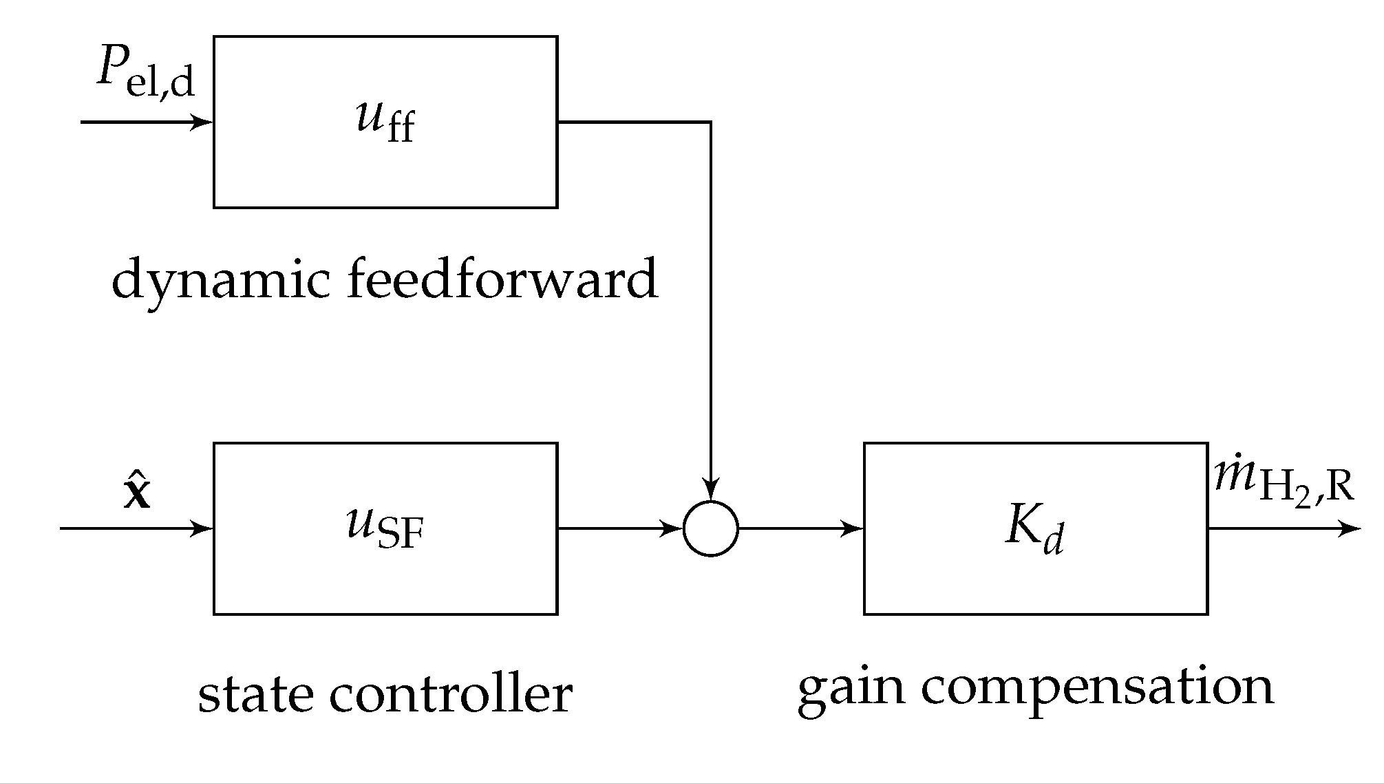
3.4. Linear State-Feedback Control

For designing this particular controller, the SOFC system in Equation (2) is approximated again by a third-order lag model (see Section 3.3), which is transformed into its controllable canonical form

$$\dot{\mathbf{x}}=\left[\begin{array}{ccc}0& 1& 0\\ 0& 0& 1\\ -a_{31}& -a_{32}& -a_{33}\end{array}\right]·\mathbf{x}+\left[\begin{array}{c}0\\ 0\\ b\end{array}\right]·u_{\mathrm{SF}}.$$

(27)

The output of this approximate system representation is given by

$$y=\left[\begin{array}{ccc}1& 0& 0\end{array}\right]·\mathbf{x}$$

(28)

with the same states $\mathbf{x}$ as in Equation (12) and the input variable $u_{\mathrm{SF}}={\dot{m}}_{{\mathrm{H}}_{2,\mathrm{SF}}}$. The controller gain ${\mathbf{k}}^{\mathrm{T}}$ included in the control law

$$u_{\mathrm{SF}}=-{\mathbf{k}}^{\mathrm{T}}·\mathbf{x}$$

(29)

was determined with the help of eigenvalue placement of the closed-loop poles

$$det(s·\mathbf{I}-(\mathbf{A}-\mathbf{b}·{\mathbf{k}}^{\mathrm{T}}))\stackrel{!}{=}\prod _{i=1}^{n=3}(s-s_{i,\mathrm{d}})$$

(30)

in the s-plane satisfying Hurwitz stability, i.e., all real parts of the eigenvalues are strictly negative according to $\Re \left\{s_{i,\mathrm{d}}\right\}<0$ and the eigenvalues are faster than the desired eigenvalues $s_{i,\mathrm{d}}$ of the open-loop system in Equation (27) [17].

To guarantee steady-state accuracy, a dynamic feedforward control

$$u_{\mathrm{ff}}={\mathbf{k}}_{\mathrm{v}}^{\mathrm{T}}·\left[\begin{array}{c}{P}_{\mathrm{el},\mathrm{d}}\\ {\dot{P}}_{\mathrm{el},\mathrm{d}}\\ {\ddot{P}}_{\mathrm{el},\mathrm{d}}\\ {\stackrel{⃛}{P}}_{\mathrm{el},\mathrm{d}}\end{array}\right]$$

(31)

was added, where ${\mathbf{k}}_{\mathrm{v}}^{\mathrm{T}}$ is determined with the numerator coefficients of the inverse transfer function of the controlled system in Equations (27)–(29).

Similar to the sliding-mode control in Section 3.3, a possible gain error resulting from model uncertainty was corrected with a static gain compensation

$$K_d={\displaystyle \frac{P_{\mathrm{el},\mathrm{d}}}{P_{\mathrm{el},\mathrm{m}}}},$$

(32)

shown in Figure 7.

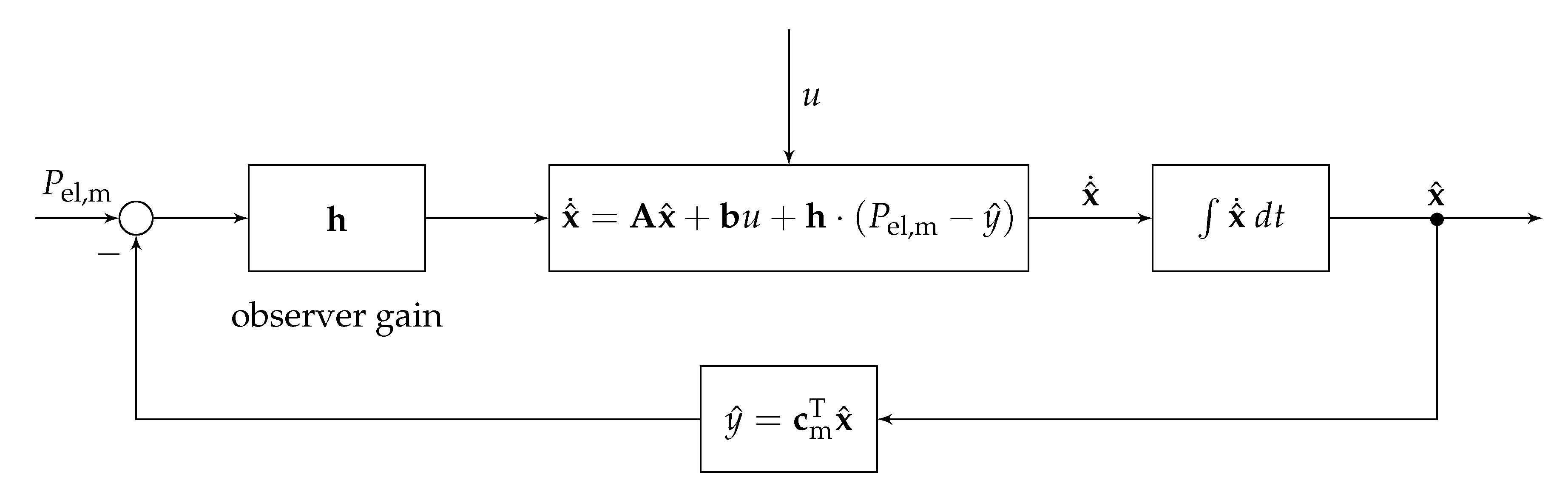
3.5. State Observer Design

For the sliding-mode controller as well as for the linear state-feedback controller, time derivatives of the measured electrical power, in Equation (12), are needed additionally. Unfortunately, they cannot be measured, so they are reconstructed by a Luenberger observer, shown in Figure 8. This observer was developed with the help of the approximate system in Equations (27) and (28).

To determine the observer gains, the principle of duality is used, which implies that the same design methodology can be applied for state-feedback controller and observer synthesis. Hence, the observer gain is also designed by placing the closed-loop poles

$$det(s·\mathbf{I}-(\mathbf{A}-\mathbf{h}·\mathbf{c}))\stackrel{!}{=}\prod _{i=1}^{n=3}(s-s_{i,\mathrm{d},\mathrm{O}})$$

(33)

in the complex left half-plane with respect to Hurwitz stability. Note that the eigenvalues $s_{i,\mathrm{d},\mathrm{O}}$ of the observed system should always be faster than the eigenvalues $s_{i,\mathrm{d}}$ of the controlled system [24].

Remark 5.

Alternative estimation approaches are Kalman filter-based derivative estimators, sliding-mode differentiators, and algebraic derivative estimation schemes [12].

4. Simulation Case Study

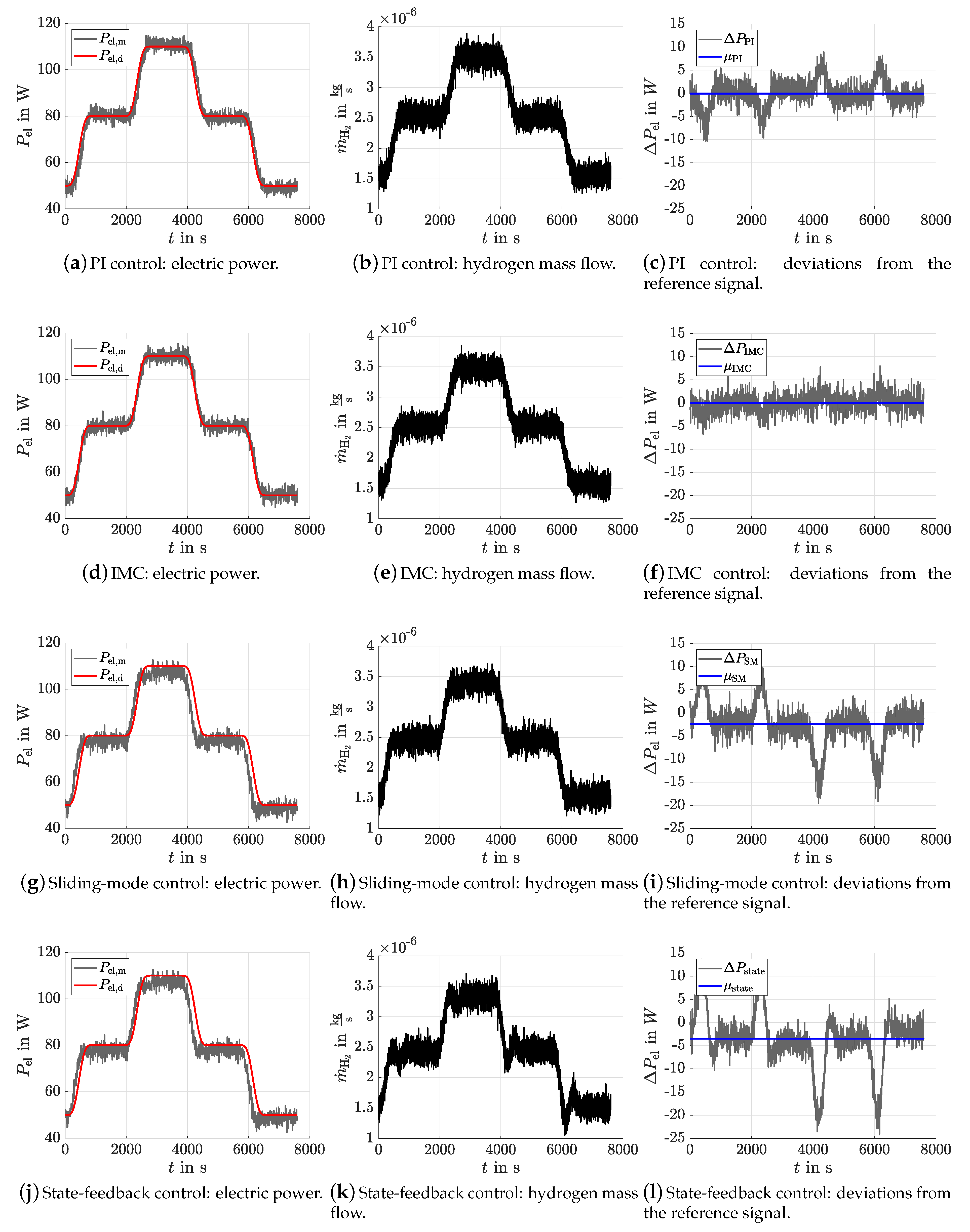
To forecast the control performance in experiments at the test rig, the four controllers of Section 3 were tested in a simulation regarding trajectory tracking and robustness against measurement noise and model uncertainties. Therefore, in the simulation, some external inputs were added with white sensor noise with a variance similar to the real measurement noise. Furthermore, the controllers were tested with $10\%$ gain and time constant deviations between the approximated system models for plant representation and control synthesis. To simulate both the transient and static behavior of each controller, the desired trajectory was chosen in such a way that it rises to a new piece-wise constant value whereby a Bernstein polynomial of order seven determines the transient phase (see Figure 9).

As a result, the IMC produces the smallest tracking error, i.e., the smallest difference between desired and simulated power, closely followed by the PI controller. The control law of the IMC is based on the inverted system model, which means that it is robust against input errors. Furthermore, the integral term inside the PI controller ensures steady-state accuracy. Here, the time constants of the PI controller are intentionally chosen very large to prevent the wind-up effects that may otherwise occur on the test rig.

Although the sliding-mode controller and the linear state-feedback controller were improved with a gain compensation, the expected gain error occurs during steady-state phases of the desired trajectory. A possible reason for this is the model mismatch between the approximated third-order lag system used for designing the sliding-mode controller and the simulated SOFC system given by a sixth-order transfer function. Note that this type of mismatch is a simple possibility to check the expected robustness of each of the presented controllers in simulations before they are applied to the test rig, where gain and time constant mismatches are further caused by neglected nonlinearities.

In the presented simulation results of the PI and IMC approaches, the manipulated variables were used more efficiently, by reducing the control amplitudes and variations in contrast to the linear state-feedback and sliding-mode controller and thus help to avoid actuator saturations at the test rig. Overall, despite the dynamic and static gain error compensation used for the sliding-mode controller and the state-feedback controller, the trajectory tracking is not as good as with the other two controllers. The design of the sliding-mode controller and the state-feedback controller could be improved with the help of an LQR design instead of pole placement. Due to the structurally implemented optimality criterion, the controller gain would then be equally optimized as opposed to the pole placement. Alternatively, an H${}_{\infty }$ norm-based design can be used for control synthesis, simultaneously improving the controller gain in terms of accounting for input limitations and maximizing the impact of the controller, while additionally accounting for process noise [25].

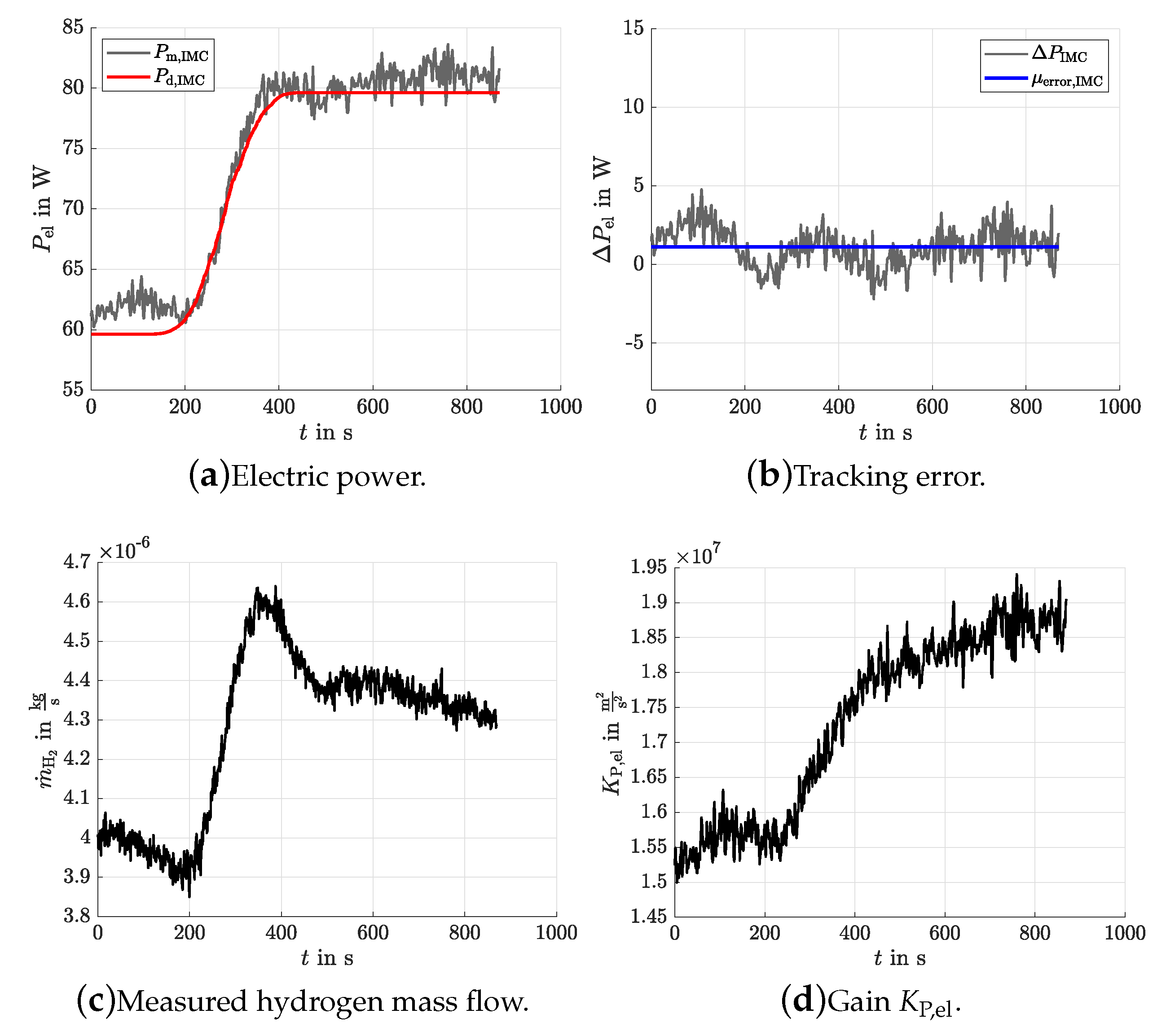
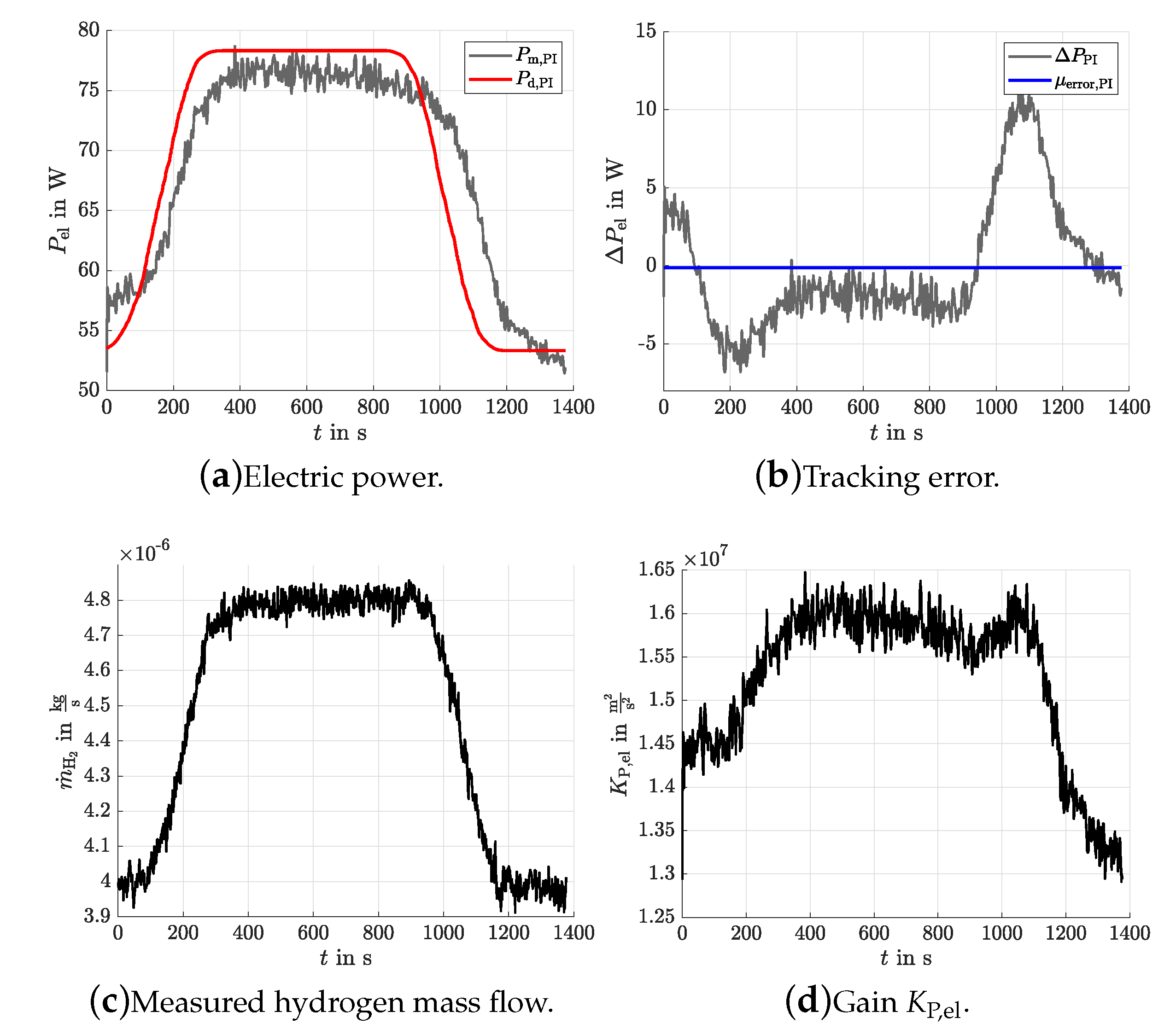
5. Experimental Validation

The PI controller and the IMC were implemented and validated in some experiments at the available test rig. An activation of the sliding-mode control and the state-feedback control in the experiment confirms the unacceptably large control amplitudes, leading to actuator saturations, which make the employed linear plant models invalid. For the experiments, the desired trajectory was slightly adjusted compared to the simulation. There, the challenge was to find a trajectory which remains in the validity domain of the model. The hydrogen mass flow has a lower limitation, which marks the minimum mass flow necessary to guarantee the desired current, here $I_{\mathrm{d}}=3\mathrm{A}$. By undershooting this limitation, the load would consume the whole hydrogen inside the fuel cell due to excessive fuel utilization, where the approximated model obviously turns invalid as soon as the current and electric power break down. The designed desired trajectory has to prevent such kind of invalidity.

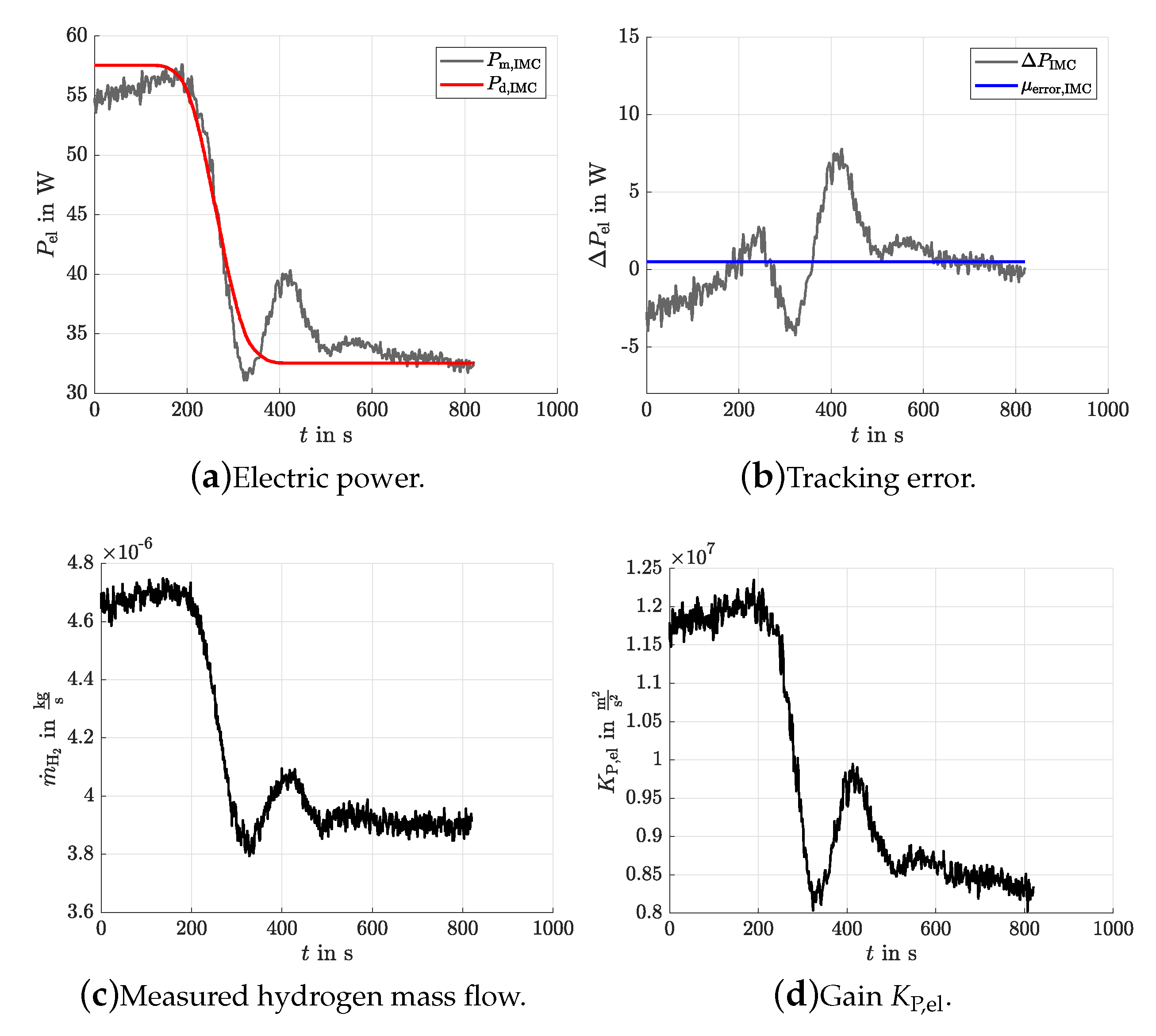
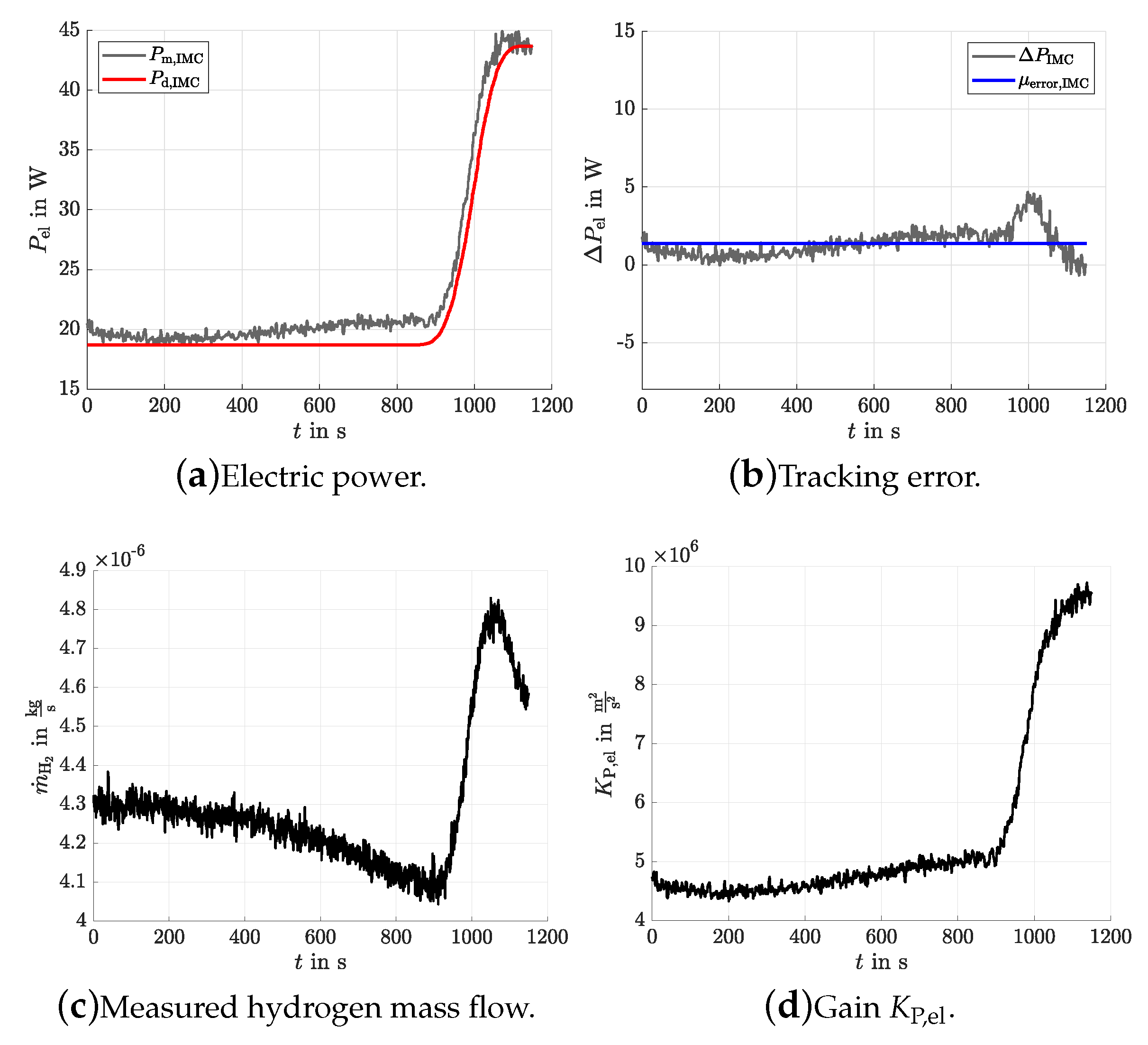
The results of the experiments are listed in

Table 1. Overview of the experimental results.

Controller	Experiment No.	${\mathit{\vartheta }}_{\mathbf{AG},\mathbf{in}}$	${\mathit{\vartheta }}_{\mathbf{CG},\mathbf{in}}$	${\mathit{\vartheta }}_{\mathbf{stack},\mathbf{min}}$	${\mathit{\vartheta }}_{\mathbf{stack},\mathbf{max}}$	${\mathit{\mu }}_{{\mathbf{P}}_{\mathbf{el}}}$	${\mathit{\sigma }}_{{\mathbf{P}}_{\mathbf{el}}}$
PI	1	$902.92\mathrm{K}$	$942.92\mathrm{K}$	$936.36\mathrm{K}$	$969.57\mathrm{K}$	$-0.12\mathrm{W}$	$4.03$
IMC	2	$910.2\mathrm{K}$	$969.42\mathrm{K}$	$937.7\mathrm{K}$	$971.04\mathrm{K}$	$1.4\mathrm{W}$	$0.92$
IMC	3	$902.62\mathrm{K}$	$986\mathrm{K}$	$936.67\mathrm{K}$	$967.19\mathrm{K}$	$1.12\mathrm{W}$	$1.19$
IMC	4	$913.13\mathrm{K}$	$958.36\mathrm{K}$	$946.89\mathrm{K}$	$971.6\mathrm{K}$	$0.497\mathrm{W}$	$2.42$

and are further shown in Figure 10 and Figure 11, Figure 12 and Figure 13, which validates the simulation results. Both the PI and IMC controllers have a good trajectory tracking accuracy with average errors of the electric power ${\mu }_{{\mathrm{P}}_{\mathrm{el}}}<3\mathrm{W}$. Because of a smaller standard deviation obtained by the IMC, it is, as for the simulation, the best controller, which is confirmed by the reduced tracking errors in transient phases. Moreover, the repetition of the experimental validation of the IMC for Experiments 2–4 shows both the reproducibility and robustness of the control accuracy for various initial power levels and, hence, confirms the robustness of the controller for a quite wide range of operating conditions despite the actual plant nonlinearities.

Besides the measured data of the electric power and its errors, the temporal variation of the gain

$$K_{\mathrm{P},\mathrm{el}}=\frac{P_{\mathrm{el},\mathrm{m}}}{{\dot{m}}_{{\mathrm{H}}_{2,\mathrm{in}}}}$$

(34)

is illustrated. It is clearly visible that a large variation of the gain of several tens of percent along the time axis occurs, which was not yet modeled. This gain variation results from unavoidable changes of the internal temperature distribution in the SOFC stack module and from variations of the cathode gas temperature which is employed to keep the stack at a constant thermal operating point despite exothermal reaction enthalpies [12]. Despite this model uncertainty resulting from actually nonlinear dynamic phenomena, the PI controller and the IMC are able to follow the desired trajectory. These model uncertainties could be analyzed in future work. Therefore, an alternative concept is to estimate this gain online and to make use of it in a generalization of the proposed PI controller and IMC towards an adaptive control approach.

Remark 6.

Furthermore, experiments showed a huge dependency between the electric power and the temperature distribution inside the stack. Due to an inhomogeneous temperature distribution with a low core temperature, the maximum electric power achieved by the cold combustion decreases. The temperature dependency has not yet been considered.

Hence, a further point for future work will be to interface the presented power controls with currently independent temperature controllers [12].

6. Conclusions and Outlook on Future Research

In this study, four different controllers for the power control of an SOFC were designed and compared with each other. A PI controller, an internal model control, a sliding-mode controller, and a linear state-feedback controller were chosen. Here, the real system was approximated by a transfer function of sixth-order (Equation (2)) using measured data from a real-life test rig. To develop each control law, this basic system was then reduced in its order by different linear time-invariant transfer functions for each case, which were transferred into controllable canonical form. All controllers were additionally modified with appropriate feedforward actions. In addition, the control law for the sliding-mode controller was modified by a stationary offset correction. A dynamic gain compensation for the linear state-feedback controller was further implemented. However, the simulation of the sliding-mode control and the linear state-feedback controller show a tracking error caused by model uncertainties, which cannot be handled by those controllers without further disturbance observer techniques. Furthermore, sliding-mode controllers and for the linear state-feedback, the time derivatives of the measured electric power were needed, so that a Luenberger observer was implemented to provide these estimates. The trajectories of each controller were simulated with the analyzed system of sixth order. To check the sensitivity numerically, white noise was added to the measured values. As a result, the IMC has the best trajectory tracking, closely followed by the PI controller. Both controllers were implemented at the test rig to perform an experimental validation. Although a temporal variation of the gain of factors up to two occurs as a model uncertainty during each of the experiments, the two controllers are able to follow the desired trajectory and confirm the results of the simulation.

In this study, the real SOFC system was approximated with the black-box transfer function estimator, which includes only the input–output behavior. The presented controllers were, hence, based on this model. This means that in future work the model should be refined, in the form of explicit current or thermal dependencies. Furthermore, the sliding-mode controller and the state-feedback controller could be improved with a compensation of the gain error. Here, it is assumed that the gain and time constants are the same in each part of the desired trajectory. However, it is possible to estimate these two parameters in real time, e.g., to implement an adaptive control. In addition, the sliding-mode controller and the state-feedback controller can be optimized with an LQR design or an H${}_{\infty }$ norm minimization, as mentioned in Section 4. However, this is not necessary for the IMC and PI controller, which are—in their current form—suitable for industrial practice. Here, the time constants of the PI controller are intentionally chosen very large to prevent the wind-up effect. This makes the designed PI controller quite slow. For future work, other anti-wind-up methods could be chosen to enhance the dynamics of the PI controller further.