Ensemble Deep Learning for Multilabel Binary Classification of User-Generated Content


1
School of Computer Science, University of Nottingham, Nottingham NG8 1BB, UK
2
Department of Computer Science and Biomedical Informatics, University of Thessaly, 35131 Lamia, Greece
*
Author to whom correspondence should be addressed.
Algorithms 2020, 13(4), 83; https://0-doi-org.brum.beds.ac.uk/10.3390/a13040083
Submission received: 14 February 2020
/
Revised: 29 March 2020
/
Accepted: 30 March 2020
/
Published: 1 April 2020
(This article belongs to the Special Issue Ensemble Algorithms and Their Applications)
Abstract
:Sentiment analysis usually refers to the analysis of human-generated content via a polarity filter. Affective computing deals with the exact emotions conveyed through information. Emotional information most frequently cannot be accurately described by a single emotion class. Multilabel classifiers can categorize human-generated content in multiple emotional classes. Ensemble learning can improve the statistical, computational and representation aspects of such classifiers. We present a baseline stacked ensemble and propose a weighted ensemble. Our proposed weighted ensemble can use multiple classifiers to improve classification results without hyperparameter tuning or data overfitting. We evaluate our ensemble models with two datasets. The first dataset is from Semeval2018-Task 1 and contains almost 7000 Tweets, labeled with 11 sentiment classes. The second dataset is the Toxic Comment Dataset with more than 150,000 comments, labeled with six different levels of abuse or harassment. Our results suggest that ensemble learning improves classification results by to .
1. Introduction
Sentiment analysis is the process by which we uncover sentiment from information. The sentiment part could refer to polarity [1], fine grained or not [2], or to pure emotion information [3,4,5]. The most common source of information for sentiment analysis is Online Social Networks (OSNs) [6,7]. User-generated content provides a unique combination of complexity and challenge for automated sentiment classification.
Automated classification refers to methods that can identify and classify information based on an inference process. Machine Learning (ML) studies these types of methods and can be generally separated in three parts: Modeling, Learning, and Classification. Given a classification task, a ML method has to create a model of the data, learn based on a set of pre-classified examples and perform a classification, as required by the task. Ensemble learning refers to the combination of finite number of ML systems to improve the classification results [8].
Various ML systems exist, most frequently characterized by the model and the training methods they employ. Artificial Neural Networks (ANNs) are one type of ML systems [9]. These networks have three layers: input, hidden, and output. In the input layer, data is initially fed into a model. The model parameters are then (re)calculated in the hidden layer, and data is classified in the output layer. Each layer consists of a set of nodes or artificial neurons which are connected to the next layer. When an ANN consists of multiple hidden layers, it is referred to as a Deep Neural Network (DNN) [10].
DNNs have been widely used in computer vision problems [11,12,13], where the goal of the classification is to identify or detect objects/items/features in an image. When the goal of the classification is to detect multiple objects in an image then the task is considered multilabel. These types of problems can be extended from computer vision to text analysis. In emotion related classification, a textual input can convey one or multiple emotions.
Traditional sentiment analysis is focused on a confined polarity or single emotion basis. Our main goal is to present the effectiveness of ensemble learning in text-based multilabel classification. In addition, we aim to trigger the researcher interest for considering multilabel emotion classification as a significant aspect regarding sentiment analysis.
Our contributions are as follows. We create and present five multilabel classification architectures and two ensembles, as well as a baseline stacked ensemble and a weighted ensemble that assigns weights based on differential evolution. Then, we highlight the effectiveness of ensemble learning in modern multilabel emotion datasets. Our results show that ensemble learning can be more effective than single DNN networks in multilabel emotion classification. In addition, we also incorporate a high-level description of the most commonly used hidden layers to introduce readers to deep-learning architectures.
The remainder of our work is formatted as described. Section 2 covers some introductory bibliography alongside state-of-the-art ensemble publications. Section 3 presents in detail our diverse DNN architectures and their individual components. Section 4 describes the ensemble methods we employed as well as some key sub-components. Section 5 presents the datasets we used and some of their properties. Section 6 details our results and potential improvements. Section 7 concludes our study with the summary and future work direction.
2. Related Work
Sentiment analysis is extensively studied since the early 2000s [14,15]. With the advent of internet, OSNs soon became the most used source for sentiment analysis [16,17]. Some of the applications of sentiment analysis are: marketing [18], politics [19], and more recently medicine [20,21]. Affective computing, as suggested by Picard [22], has sparked the interest in the specific emotion analysis of texts [3,23].
Machine learning has been successfully applied to sentiment analysis of texts [24,25,26]. ML methods that have been used for sentiment analysis are: Support Vector Machines [27,28], Multinomial Naïve Bayes [29] and Decision Trees [30], while DNNs were introduced more recently [31,32].
DNNs can be used in text related applications as well. In [33] Severyn and Moschitti rerank short texts in pairs and present the per pair relation without manual feature engineering. Lai et al. [34] perform unsupervised text classification and highlight key text components in the process via a recurrent convolutional neural network. The authors of [35] perform a named entity recognition task and generate relevant word embedding with two separate DNNs. Text generation is addressed via a recurrent neural network in [36] and an extensively trained model outperforms the best non-NN models. Sentiment classification of textual sources had its own fair share of DNN implementations [31,32,37].
Learning ensembles have been used to combine different types of information, such as audio video and text towards sentiment and emotional classification [38]. Araque et al. use an ensemble of classifiers that combines features and word vectors [39] for sentiment classification with greater than 80% F-Score. A soft voting ensemble is used in [40] for topic-document and document classification the results suggesting a significant improvement over single-model methods. The authors of [41] use a stacked two-layer ensemble of CNN to predict the message level sentiment of Tweets, with the addition of a distant supervision phase. A pseudo-ensemble, essentially an ensemble of similar models trained on noisy sub-data, is used for sentiment analysis purposes in [42], but is ineffective for regression classification problems.
Multilabel classification problems assign multiple classes per item. Such problems are frequently observed in the field of computer vision [43,44,45]. With regards to multilabel text-based sentiment analysis, Chen et al. [46] propose an ensemble of a convolution neural network and a recurrent neural network for feature extraction and class prediction correspondingly. The authors of [47] propose a Maximum Entropy model for multilabel classification of short texts found in OSNs. Furthermore, they present an emotion per term lexicon as generated by the model, based on six basic emotions. However, they calculate a micro averaged F1 based on the top emotions per item, essentially converting each weighted label to binary format. Johnson and Zhang [48] present a combination of word order and bag of words in a CNN architecture and point out the threshold sensitivity in multilabel classification.
3. DNN Architectures
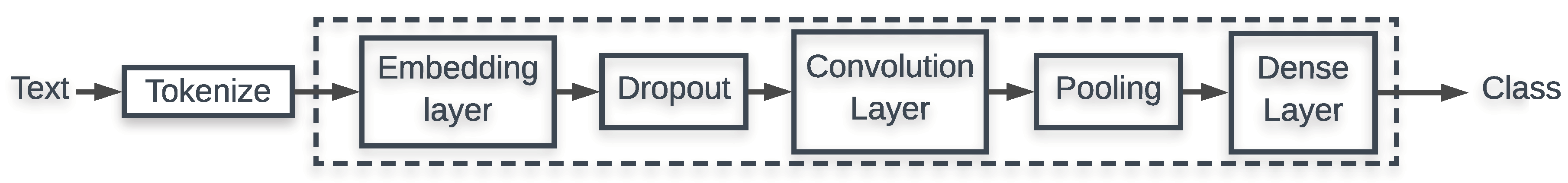
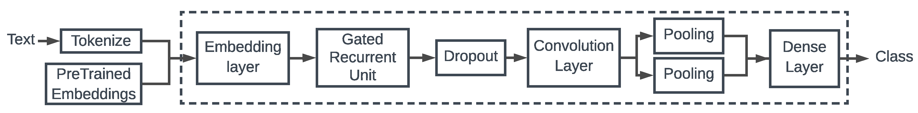
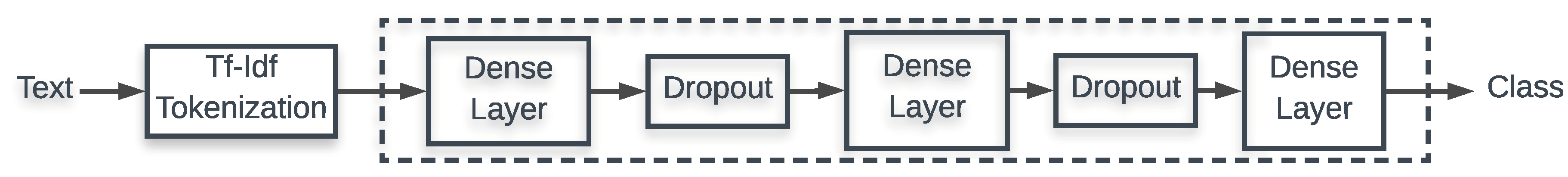
We create five different DNNs, with diverse architectures, suited to a multilabel classification problem. Model 1, Figure 1, is a simple CNN with one fully connected layer. Model 2, Figure 2, combines a Gated Recurrent Unit and a Convolution layer, similar to [49]. Model 3, Figure 3, uses Term Frequency Inverse Document Frequency Embeddings and three fully connected layers, inspired by [50]. Model 4, Figure 4, architecture is based on the top performing single model of the Toxic Comment Classification Challenge in Kaggle https://www.kaggle.com/c/jigsaw-toxic-comment-classification-challenge. Model 5, Figure 5, combines uni/bi/tri grams follow by three interconnected CNN processes, as presented in [51]. Each of the modules used in these models is presented in this section.
3.1. Pre-Processing
For each dataset used, we perform a pre-processing that includes term lemmatization and stemming, lowercase conversion, removal of non-pure text elements (such as Uniform Resource Locators or Emotes), stop word filtering and frequency-based term exclusion. Although some information is lost, extensive term filtering is shown to improve classification results [52].
3.2. Tokenization
Tokenization is performed on a term level for all the five methods presented. Each term is represented by a unique token. Further linguistic elements such as abbreviations and negations are cleaned, returned to their canonical form, and get assigned a token. For example, commonly used negation ‘don’t’ is tokenized to ‘do’, ‘not’.
3.3. Embedding
We assign a vector value for each token in a sentence, e.g., based on the order they appeared in our corpus, and we create a vector of numerical values. The mapping of word tokens to numerical values of vectors is referred to as embedding. There are various ways of creating word embeddings. Term Frequency-Inverse Document Frequency Tokenization creates a matrix of TF-IDF features which are used to create the embedding. Every sentence is converted to a single dimension vector of numerical elements regardless of the tokenization method. To address variable sentence length, we define a large vector length and we fill the numerical vector with zeroes, a process known as padding. Most common and effective word embedding methods are created based on term co-occurrence throughout a large corpus [53,54].
3.4. Dropout
Neural networks are prone to overfitting. Overfitting is essentially the exhaustive training of the model in a certain set of data, so much that the model fails to generalize. As a result, the model cannot effectively work with new unknown data. A solution to overfitting is to train multiple models and combine their output afterwards, which is highly inefficient.
Srivastava et al. [55] proposed randomly dropping neural units from the network during the training phase. Their results suggested an improvement of the regularization on diverse datasets. Spatial dropout refers to the exact same process, performed over a single axis of elements, rather than random neural units over each layer. Furthermore, dropout has a significant potential to reduce overfitting and provide improvements over other regularization strategies such as L-regularization and soft-weight sharing [56].
3.5. LSTM and Gated Recurrent Unit
A feed-forward neural network has a unidirectional processing path, from input to hidden layer to output. A recurrent network can have information travelling both directions by using feedback loops. Computations derived from earlier input are fed back into the network, imitating human memory. In essence, a recurrent neural network is a chain of identical neural networks that transfer the derived knowledge from one to another. That chain creates learning dependencies that decay mainly due to the size of the chained network.
Hochreiter and Schmidhuber [57] proposed Long Short-Term Memory networks to counter that decay. The novel unit of the LSTM architecture is the memory cell that forgets or remembers the information passed from the previous chain link. The Gated Recurrent Unit of Model 2 was introduced by Cho et al. [58]. Its architecture is similar to LSTM units, but with the absence of an output gate. It is shown that GRU networks perform well on Natural Language Processing tasks [59].
3.6. Convolution
The convolution layer receives as input a tensor, which is convolved and its output, the feature map, is passed to the next layer. A tensor is a mathematical object that describes a mapping of an input set of objects to an output set. Therefore The convolution layers in all models are one-dimensional, with a convolution window of size 3 and an output space dimensionality of 128. The only exception is Model 5, where the convolution windows is different for each layer to provide a differentiated architecture. The primary focus of this layer is to extract features from the input data by preserving the spatial relationship between terms.
3.7. Pooling and Flattening
A pooling layer allows us to reduce the dimensionality of the processed data by keeping only the most important information. Common types of pooling are max, average and sum. The respective operation, per pooling type, is performed in a predefined window of the feature map. A pooling layer reduces the computational cost of the network, leads to scale invariant representations and counters small feature map transformations. Finally, by having a reduced number of features, we decrease the probability of overfitting. Various pooling types were used, based on the architecture. Model 1 uses a single global max pooling layer; the global parameter is outputting the single most important feature of the feature map instead of a feature window. Model 2 uses a combination of global max and a global average pooling layers, while Model 4 uses the local pooling equivalents. Model 5 uses three local max pooling layers, one for each convolution.
The flattening layer on the other hand reduces the dimensionality of the input to one. For example, a feature map with dimensions when flattened would produce a one-dimensional vector with 20 elements. The flattening layer passes the most important features of the input data to a fully connected dense layer comprised of the classification neurons.
3.8. Dense
The dense layer is comprised by fully connected neurons both forward and backward. Every element of the input is connected with every neuron of this layer. In four out of five models, a dense layer can be seen at the end of the pipeline. The number of neurons in these layers is the number of classes in our dataset. For the third model, where TF-IDF tokenization takes place, we chose a simple DNN with 3 fully connected layer, which decreasing number of neurons for each subsequent layer. DNNs with multiple dense fully connected layers is shown to perform better than shallow DNNs [60].
3.9. Classification
The output of our model is a multilabel classification vector. Each of the neurons in the final dense layer of the models interact with the classes of the dataset and provide a decimal value (ranging from 0 to 1) which is then rounded for each class. The number of classes defines the number of fully connected neurons in the final dense layer.
4. Ensembles
We previously mentioned that a method to counter overfitting is to train multiple models and then combine their outputs. Ensemble learning combines the single-model outputs to improve predictions and generalization. Ensemble learning improves upon three key aspects of learning, statistics, computation and representation [61]. From a statistics perspective, ensemble methods reduce the risk of data miss-representation, by combining multiple models we reduce the risk of employing a single model trained with biased data. While most learning algorithms search locally for solutions which in turn confines the optimal solution, ensemble methods can execute random seed searches with variable start points with less computational resources. A single hypothesis rarely represents the target function, but an aggregation of multiple hypothesis, as found in ensembles, can better approximate the target function.
We present two ensemble architectures, stacked and weighted [51]. Other popular ensemble methods include AdaBoost, Random Forest and Bagging [62]. Stacked ensembles are the simplest yet one of the most effective ensemble methods, widely used in a variety of applications [63,64]. Stacked ensemble acts as our baseline ensemble, compared with our proposed weighted ensemble based on differential evolution, a meta-heuristic weight optimization method. Meta-heuristic weighted ensembles have achieved remarkable results in single label text classification [65,66].
4.1. Stacked
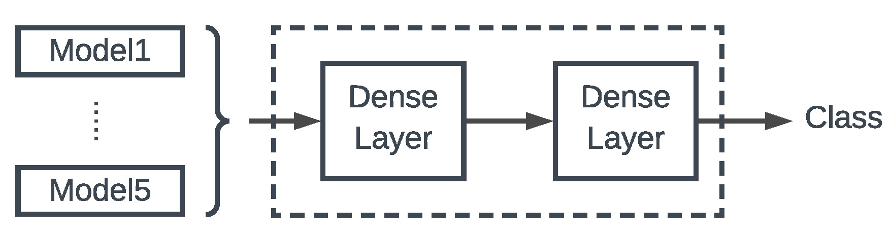
The main idea behind stacked ensembles is to combine a set of trained models through training of another model (meta-model). The output predictions of the meta-model are based on the training of the model outputs, Algorithm 1. In our implementation we fit the models output into a DNN with two hidden dense layers, Figure 6.
| Algorithm 1 Stacked Ensemble Pseudo-code |
|
The outputs of the models are merged with the concatenation function of Keras https://keras.io/. The input of the concatenation is a fixed size output tensor of each model. The output of the concatenation is a single tensor, which is then used as an input to the fully connected layer. A second fully connected layer follows similar to the final dense layer on each model.
4.2. Weighted
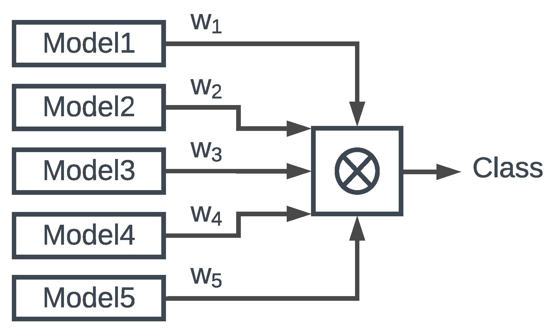
The weighted ensemble has a similar philosophy behind it. Instead of equally merging the outputs, we merge the outputs by co-calculating a weight. Given a set of weighted tensors and a vector-like object, we sum the product of tensor elements over a single axis, as specified by the one-dimensional vector, Figure 7.
The ‘fitting’ process of the second ensemble is a heuristic process for the best possible weights combination, i.e., looking for the global minimum of a multivariate function. We propose differential evolution [67] to scan the large space of five distinct weights, Algorithm 2.
| Algorithm 2 Differential Evolution Pseudo-code |
|
5. Datasets
For our comparison, we require datasets with binary multilabel categorization. We identified two modern datasets, Semeval 2018 Task 1 Dataset (SEM2018) https://competitions.codalab.org/competitions/17751 and Toxic Comments Dataset from Kaggle (TOXIC) https://www.kaggle.com/c/jigsaw-toxic-comment-classification-challenge.
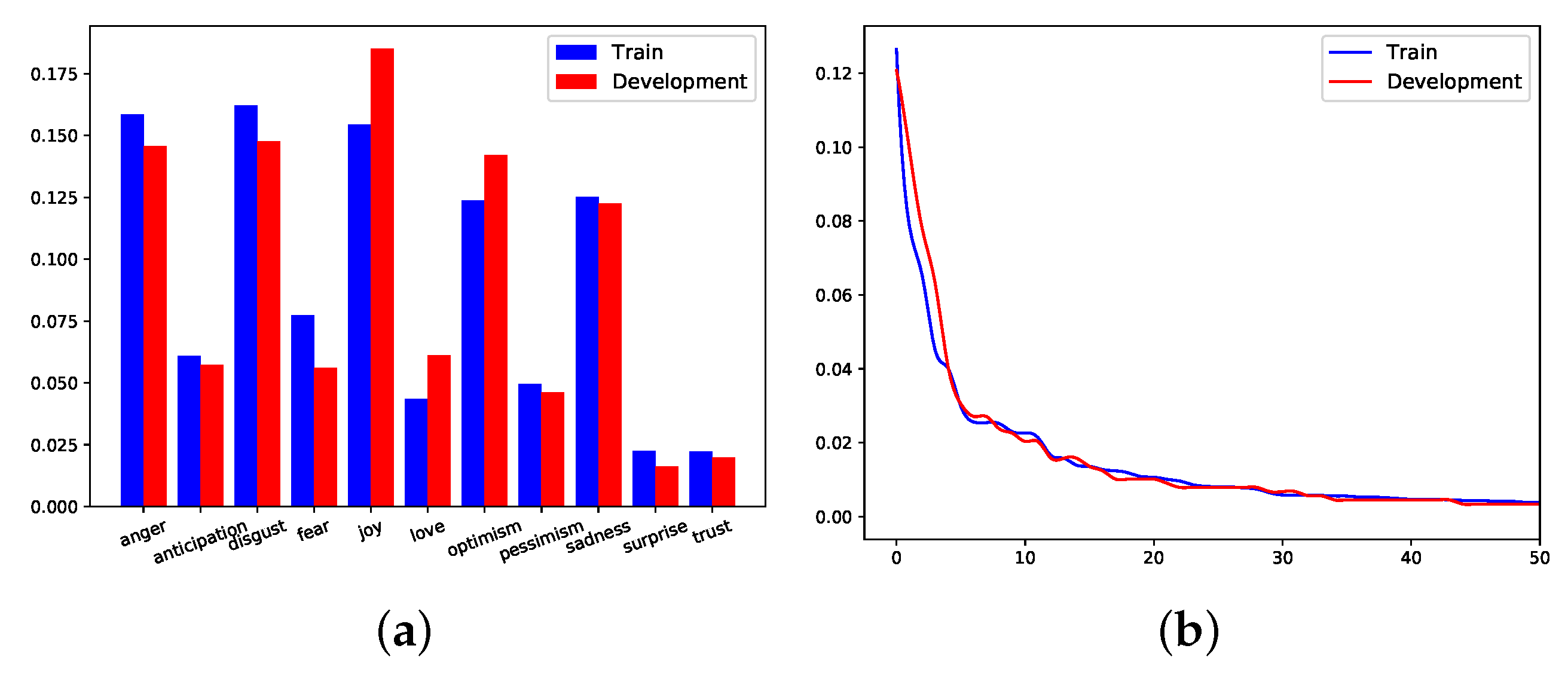
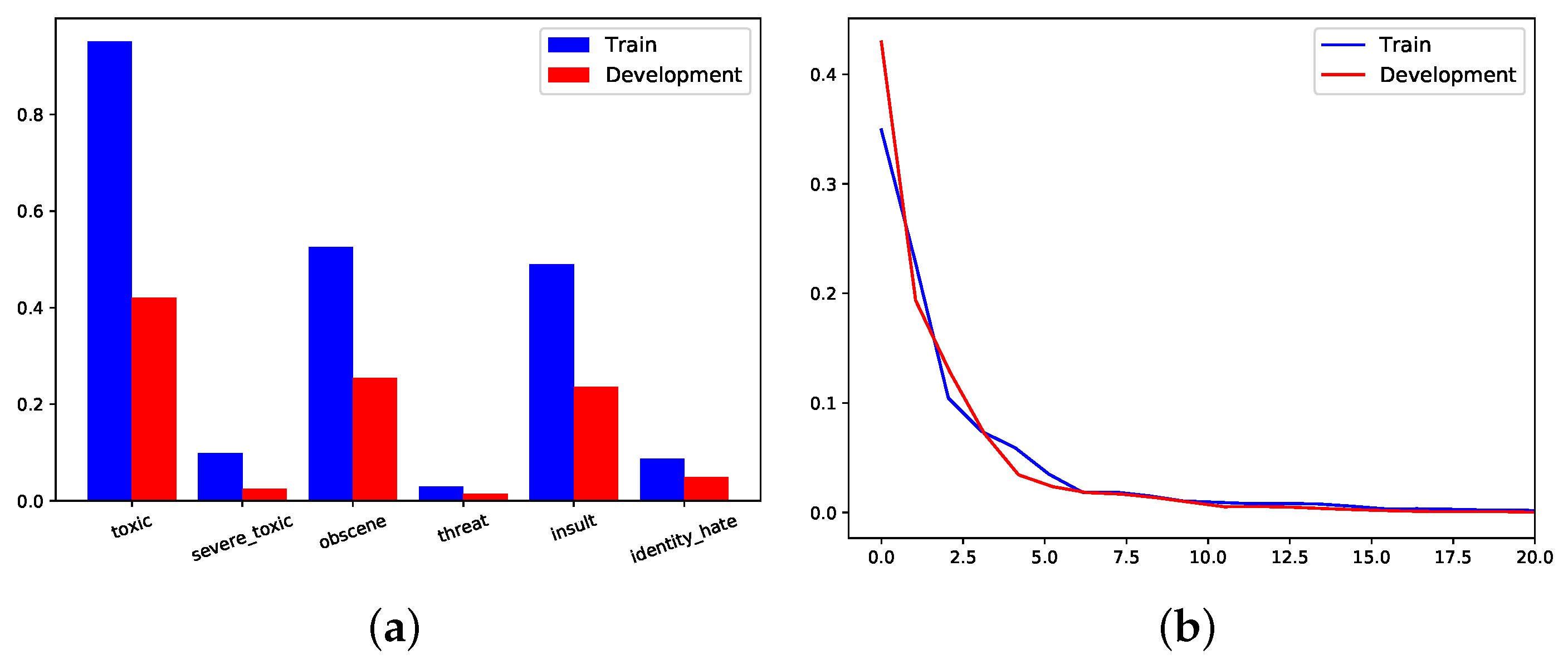
Both datasets exhibit a level of class imbalance, Figure 8a and Figure 9a. However, they are different not only in context, where SEM2018 is based on Twitter and TOXIC in Wikipedia, but also in the properties of the actual text. The sentence length, after the source is cleaned, is different from the original mainly due to the removal of infrequent terms, Table 1. We discussed before that the dimensions of our term embeddings need to be low. We reduced the dimension by removing the terms that appear no more than 10 times, alongside a tailored stop term removal.
5.1. Semeval 2018
The SEM2018 Train is a collection of 6838 Tweets with emotion labeling of 11 classes. The classes are: anger, anticipation, disgust, fear, joy, love, optimism, pessimism, sadness, surprise and trust. Some examples of Tweets included in SEM2018 are:
- Whatever you decide to do make sure it makes you happy.
- Nor hell a fury like a woman scorned—William Congreve
- chirp look out for them Cars coming from the Wesszzz
- Manchester derby at home revenge
The Development dataset consists of 886 Tweets with the 11 aforementioned classes and their respective labels. The class distribution in Train dataset is skewed in favor of five emotions, anger, disgust, joy, optimism, and sadness. The same class distribution is evident in the Development dataset, which is dominated by the same five emotions, Figure 8a.
SEM2018 contains 329 unique class combinations. The frequency of these unique combinations follows a power law distribution for both Train and Development datasets Figure 8b. The most frequent class combination for Train and Development was: anger and disgust, followed by joy and optimism. One third of the class combinations appears only once and often combine contradiction emotions, such as joy and sadness.
5.2. Toxic Comments
The Toxic dataset consists of two datasets as well, Train and Development. Train dataset consists of 159,571 unique comments labeled with 6 different types of toxicity: toxic, severe_toxic, obscene, threat, insult and identity_hate. Some example of comments are:
- I don’t anonymously edit articles at all.
- Dear god this site is horrible.
- Please pay special attention on this
- Cant sing for s**t though.
The Development dataset consists of 63,978 toxic comments with the same classes and their respective labels. The class distribution is heavily skewed towards toxic, obscene and insult, in both Train and Development, Figure 9a.
TOXIC Train includes 29 unique class combinations, while Development has 21. Both frequencies follow a power law distribution, similar to SEM2018, Figure 9b. The most common class combinations for Train and Development are: obscene and insult, obscene only and insult only. The most uncommon class combinations included threat and severe_toxic classes. Out of 29 unique classes for Train 12 have more than 100 occurrences, while out of 21 unique class combinations of Development 7 appear more than 100 times.
6. Results
The accuracy scores are validated via 10-fold validation. The baseline neural network (NN) model [68] expectedly under-performs [69]. For the SEM2018 datasets, both ensembles outperform each individual model. The stacked ensemble provides the best results in the Train subset while the weighted ensemble marginally outperforms stacked ensemble in the Development subset, Table 2. The accuracy of both ensembles is limited, to a degree, by the inherit bias of the dataset. The performance of our ensembles outperforms all submitted models in the Codalab Competition https://competitions.codalab.org/competitions/17751#results.
The baseline NN performed better in TOXIC dataset. NN performance is boosted by the big number of unclassified elements in the dataset, Table 3, more than of the samples as seen in Figure 9b. TOXIC dataset included more than 25,000 unique terms before cleaning. The number of unique terms affects the length of the tokenization and subsequently the dimension of the embedding. The required dimension reduction reduced the training time of each model but affected its performance. Our best performing model is in the op 35% of the Kaggle Competition submissions https://www.kaggle.com/c/jigsaw-toxic-comment-classification-challenge/leaderboard but more than 1% worse when compared to the top performing one.
Our ensemble methods improved upon single models in six out of eight cases. The classification accuracy is improved by at least one of the ensembles across both datasets. The ensembles for SEM2018 dataset performed excellently compared to other architectures. On the other hand, the extensive data cleaning of TOXIC -requirement due to computation/time constraints- hindered the performance of our models and their ensembles. Given the heavy class imbalance and the cleaning of TOXIC, the achieved accuracy of 97+% is decent. The baseline stacked ensemble under-performed our proposed weighted ensemble in three out of four cases.
All the models presented, and in extent their ensembles, can be further improved by a range of techniques. Test augmentation [70], hyperparameter optimization [71], bias reduction [72] and tailored emotional embeddings [4,73] are some techniques that could further improve the generalization capabilities of our networks. However, the computational load over multiple iterations is extensive, as the most complex models required hours of training per epoch and dataset.
7. Conclusions
We demonstrated that ensemble learning can improve the classification accuracy in multilabel text classification applications. We created and tested five different deep-learning architectures capable of handling multilabel binary classification tasks.
Our five DNN architectures were ensembled via two methods, stacked and weighted, and tested in two different datasets. The datasets used provide a similar multilabel classification but vary in size, term distribution and term frequency. The classification accuracy was improved by the ensemble models in both tasks. Our proposed weighted ensemble outperformed the baseline stacked ensemble in of cases by to . Hyperparameter tuning, supervised or unsupervised, could further improve the results but with a heavy computational load, since each hyperparameter iteration requires the re-training/re-calculation of the ensemble.
Moving forward we aim to explore the creation and use of tailored emotional embeddings concatenated with word embeddings. Additionally, we are currently developing new data augmentation methods, tailored to text datasets. We are also exploring multilabel regression ensembles and architectures that could be considered to be the refinement of binary classification, whether multilabel or not.
Author Contributions
Conceptualization, G.H. and I.A.; methodology, G.H.; software, G.H.; validation, G.H.; formal analysis, G.H.; investigation, G.H.; resources, G.H.; data curation, G.H.; writing—original draft preparation, G.H. and I.A.; writing—review and editing, G.H., I.A. and D.M.; visualization, G.H.; supervision, I.A. and D.M.; funding acquisition, D.M. All authors have read and agreed to the published version of the manuscript.
Funding
This research was funded by Engineering and Physical Sciences Research Council grant number EP/M02315X/1: “From Human Data to Personal Experience”.
Conflicts of Interest
The authors declare no conflict of interest.
References
- Barbieri, F.; Basile, V.; Croce, D.; Nissim, M.; Novielli, N.; Patti, V. Overview of the Evalita 2016 Sentiment Polarity Classification Task. 2016. Available online: http://ceur-ws.org/Vol-1749/paper_026.pdf (accessed on 31 March 2020).
- Tang, F.; Fu, L.; Yao, B.; Xu, W. Aspect based fine-grained sentiment analysis for online reviews. Inf. Sci. 2019, 488, 190–204. [Google Scholar] [CrossRef]
- Poria, S.; Chaturvedi, I.; Cambria, E.; Hussain, A. Convolutional MKL based multimodal emotion recognition and sentiment analysis. In Proceedings of the 2016 IEEE 16th International Conference on Data Mining (ICDM), Barcelona, Spain, 12–15 December 2016; pp. 439–448. [Google Scholar]
- Haralabopoulos, G.; Wagner, C.; McAuley, D.; Simperl, E. A multivalued emotion lexicon created and evaluated by the crowd. In Proceedings of the 2018 Fifth International Conference on Social Networks Analysis, Management and Security (SNAMS), Valencia, Spain, 15–18 October 2018; pp. 355–362. [Google Scholar]
- Haralabopoulos, G.; Simperl, E. Crowdsourcing for beyond polarity sentiment analysis a pure emotion lexicon. arXiv 2017, arXiv:1710.04203. [Google Scholar]
- Go, A.; Bhayani, R.; Huang, L. Twitter sentiment classification using distant supervision. CS224N Proj. Rep. Stanf. 2009, 1, 2009. [Google Scholar]
- Tian, Y.; Galery, T.; Dulcinati, G.; Molimpakis, E.; Sun, C. Facebook sentiment: Reactions and emojis. In Proceedings of the Fifth International Workshop on Natural Language Processing for Social Media, Valencia, Spain, 3 April 2017; pp. 11–16. [Google Scholar]
- Zhang, C.; Ma, Y. Ensemble Machine Learning: Methods and Applications; Springer: Berlin/Heidelberg, Germany, 2012. [Google Scholar]
- Zurada, J.M. Introduction to Artificial Neural Systems; West Publishing Company St. Paul: Eagan, MN, USA, 1992; Volume 8. [Google Scholar]
- Glorot, X.; Bengio, Y. Understanding the difficulty of training deep feedforward neural networks. In Proceedings of the Thirteenth International Conference on Artificial Intelligence and Statistics, Sardinia, Italy, 13–15 May 2010; pp. 249–256. [Google Scholar]
- Mollahosseini, A.; Chan, D.; Mahoor, M.H. Going deeper in facial expression recognition using deep neural networks. In Proceedings of the 2016 IEEE Winter Conference on Applications of Computer Vision (WACV), Lake Placid, NY, USA, 7–9 March 2016; pp. 1–10. [Google Scholar]
- Havaei, M.; Davy, A.; Warde-Farley, D.; Biard, A.; Courville, A.; Bengio, Y.; Pal, C.; Jodoin, P.M.; Larochelle, H. Brain tumor segmentation with deep neural networks. Med. Image Anal. 2017, 35, 18–31. [Google Scholar] [CrossRef] [PubMed] [Green Version]
- Abbaspour-Gilandeh, Y.; Molaee, A.; Sabzi, S.; Nabipur, N.; Shamshirband, S.; Mosavi, A. A Combined Method of Image Processing and Artificial Neural Network for the Identification of 13 Iranian Rice Cultivars. Agronomy 2020, 10, 117. [Google Scholar] [CrossRef] [Green Version]
- Nasukawa, T.; Yi, J. Sentiment analysis: Capturing favorability using natural language processing. In Proceedings of the 2nd International Conference on Knowledge Capture, Sanibel Island, FL, USA, 23–25 October 2003; pp. 70–77. [Google Scholar]
- Yi, J.; Nasukawa, T.; Bunescu, R.; Niblack, W. Sentiment analyzer: Extracting sentiments about a given topic using natural language processing techniques. In Proceedings of the Third IEEE International Conference on Data Mining, Melbourne, FL, USA, USA, 19–22 November 2003; pp. 427–434. [Google Scholar]
- Agarwal, A.; Xie, B.; Vovsha, I.; Rambow, O.; Passonneau, R. Sentiment analysis of twitter data. In Proceedings of the Workshop on Language in Social Media (LSM 2011), Portland, OR, USA, 23 June 2011; pp. 30–38. [Google Scholar]
- Pak, A.; Paroubek, P. Twitter as a corpus for sentiment analysis and opinion mining. LREc 2010, 10, 1320–1326. [Google Scholar]
- Cvijikj, I.P.; Michahelles, F. Understanding social media marketing: A case study on topics, categories and sentiment on a Facebook brand page. In Proceedings of the 15th International Academic MindTrek Conference: Envisioning Future Media Environments, Tampere, Finland, 28–30 September 2011; pp. 175–182. [Google Scholar]
- Mullen, T.; Malouf, R. A Preliminary Investigation into Sentiment Analysis of Informal Political Discourse. In Proceedings of the AAAI Spring Symposium: Computational Approaches to Analyzing Weblogs, Stanford, CA, USA, 27–29 March 2006; pp. 159–162. [Google Scholar]
- Denecke, K.; Deng, Y. Sentiment analysis in medical settings: New opportunities and challenges. Artif. Intell. Med. 2015, 64, 17–27. [Google Scholar] [CrossRef]
- Zhang, Y.; Chen, M.; Huang, D.; Wu, D.; Li, Y. iDoctor: Personalized and professionalized medical recommendations based on hybrid matrix factorization. Future Gener. Comput. Syst. 2017, 66, 30–35. [Google Scholar] [CrossRef]
- Picard, R.W. Affective Computing; MIT Press: Cambridge, MA, USA, 2000. [Google Scholar]
- Cambria, E. Affective computing and sentiment analysis. IEEE Intell. Syst. 2016, 31, 102–107. [Google Scholar] [CrossRef]
- Alm, C.O.; Roth, D.; Sproat, R. Emotions from text: Machine learning for text-based emotion prediction. In Proceedings of the Conference on Human Language Technology and Empirical Methods in Natural Language Processing, Vancouver, BC, Canada, 6–8 October 2005; pp. 579–586. [Google Scholar]
- Boiy, E.; Hens, P.; Deschacht, K.; Moens, M.F. Automatic Sentiment Analysis in On-line Text. In Proceedings of the ELPUB2007 Conference on Electronic Publishing, Vienna, Austria, 13–15 June 2007; pp. 349–360. [Google Scholar]
- Asghar, M.Z.; Subhan, F.; Imran, M.; Kundi, F.M.; Shamshirband, S.; Mosavi, A.; Csiba, P.; Varkonyi-Koczy, A.R. Performance evaluation of supervised machine learning techniques for efficient detection of emotions from online content. arXiv 2019, arXiv:1908.01587. [Google Scholar]
- Chaffar, S.; Inkpen, D. Using a heterogeneous dataset for emotion analysis in text. In Proceedings of the Canadian Conference on Artificial Intelligence, St. John’s, NL, Canada, 25–27 May 2011; pp. 62–67. [Google Scholar]
- Sidorov, G.; Miranda-Jiménez, S.; Viveros-Jiménez, F.; Gelbukh, A.; Castro-Sánchez, N.; Velásquez, F.; Díaz-Rangel, I.; Suárez-Guerra, S.; Trevino, A.; Gordon, J. Empirical study of machine learning based approach for opinion mining in tweets. In Proceedings of the Mexican international conference on Artificial intelligence, San Luis Potosí, Mexico, 27 October–4 November 2012; pp. 1–14. [Google Scholar]
- Boiy, E.; Moens, M.F. A machine learning approach to sentiment analysis in multilingual Web texts. Inf. Retr. 2009, 12, 526–558. [Google Scholar] [CrossRef]
- Annett, M.; Kondrak, G. A comparison of sentiment analysis techniques: Polarizing movie blogs. In Proceedings of the Conference of the Canadian Society for Computational Studies of Intelligence, Windsor, ON, Canada, 28–30 May 2008; pp. 25–35. [Google Scholar]
- Dos Santos, C.; Gatti, M. Deep convolutional neural networks for sentiment analysis of short texts. In Proceedings of the 25th International Conference on Computational Linguistics (COLING 2014), Dublin, Ireland, 23–29 August 2014; pp. 69–78. [Google Scholar]
- Wang, X.; Jiang, W.; Luo, Z. Combination of convolutional and recurrent neural network for sentiment analysis of short texts. In Proceedings of the 26th International Conference on Computational Linguistics (COLING 2016), Osaka, Japan, 11–16 December 2016; pp. 2428–2437. [Google Scholar]
- Severyn, A.; Moschitti, A. Learning to rank short text pairs with convolutional deep neural networks. In Proceedings of the 38th international ACM SIGIR Conference on Research and Development in Information Retrieval, Santiago, Chile, 9–13 August 2015; pp. 373–382. [Google Scholar]
- Lai, S.; Xu, L.; Liu, K.; Zhao, J. Recurrent convolutional neural networks for text classification. In Proceedings of the Twenty-Ninth AAAI Conference on Artificial Intelligence, Austin, TX, USA, 25–30 January 2015. [Google Scholar]
- Wu, Y.; Jiang, M.; Lei, J.; Xu, H. Named entity recognition in Chinese clinical text using deep neural network. Stud. Health Technol. Inform. 2015, 216, 624. [Google Scholar] [PubMed]
- Sutskever, I.; Martens, J.; Hinton, G.E. Generating text with recurrent neural networks. In Proceedings of the 28th International Conference on Machine Learning (ICML-11), Bellevue, WC, USA, 28 June–2 July 2011; pp. 1017–1024. [Google Scholar]
- Tang, D.; Qin, B.; Liu, T. Document modeling with gated recurrent neural network for sentiment classification. In Proceedings of the 2015 Conference on Empirical Methods in Natural lAnguage Processing, Lisbon, Portugal, 17–21 September 2015; pp. 1422–1432. [Google Scholar] [CrossRef]
- Poria, S.; Peng, H.; Hussain, A.; Howard, N.; Cambria, E. Ensemble application of convolutional neural networks and multiple kernel learning for multimodal sentiment analysis. Neurocomputing 2017, 261, 217–230. [Google Scholar] [CrossRef]
- Araque, O.; Corcuera-Platas, I.; Sanchez-Rada, J.F.; Iglesias, C.A. Enhancing deep learning sentiment analysis with ensemble techniques in social applications. Expert Syst. Appl. 2017, 77, 236–246. [Google Scholar] [CrossRef]
- Xu, S.; Liang, H.; Baldwin, T. Unimelb at semeval-2016 tasks 4a and 4b: An ensemble of neural networks and a word2vec based model for sentiment classification. In Proceedings of the 10th International Workshop on Semantic Evaluation (SemEval-2016), San Diego, CA, USA, 16–17 June 2016; pp. 183–189. [Google Scholar] [CrossRef]
- Deriu, J.; Gonzenbach, M.; Uzdilli, F.; Lucchi, A.; Luca, V.D.; Jaggi, M. Swisscheese at semeval-2016 task 4: Sentiment classification using an ensemble of convolutional neural networks with distant supervision. In Proceedings of the 10th International Workshop on Semantic Evaluation, San Diego, CA, USA, 16–17 June 2016; pp. 1124–1128. [Google Scholar]
- Bachman, P.; Alsharif, O.; Precup, D. Learning with pseudo-ensembles. Adv. Neural Inf. Process. Syst. 2014, 27, 3365–3373. [Google Scholar]
- Gong, Y.; Jia, Y.; Leung, T.; Toshev, A.; Ioffe, S. Deep convolutional ranking for multilabel image annotation. arXiv 2013, arXiv:1312.4894. [Google Scholar]
- Cakir, E.; Heittola, T.; Huttunen, H.; Virtanen, T. Polyphonic sound event detection using multi label deep neural networks. In Proceedings of the 2015 International Joint Conference on Neural Networks (IJCNN), Killarney, Ireland, 12–17 July 2015; pp. 1–7. [Google Scholar]
- Huang, Y.; Wang, W.; Wang, L.; Tan, T. Multi-task deep neural network for multi-label learning. In Proceedings of the 2013 IEEE International Conference on Image Processing, Melbourne, VIC, Australia, 15–18 September 2013; pp. 2897–2900. [Google Scholar]
- Chen, G.; Ye, D.; Xing, Z.; Chen, J.; Cambria, E. Ensemble application of convolutional and recurrent neural networks for multi-label text categorization. In Proceedings of the 2017 International Joint Conference on Neural Networks (IJCNN), Anchorage, AK, USA, 14–19 May 2017; pp. 2377–2383. [Google Scholar]
- Li, J.; Rao, Y.; Jin, F.; Chen, H.; Xiang, X. Multi-label maximum entropy model for social emotion classification over short text. Neurocomputing 2016, 210, 247–256. [Google Scholar] [CrossRef]
- Johnson, R.; Zhang, T. Effective use of word order for text categorization with convolutional neural networks. arXiv 2014, arXiv:1412.1058. [Google Scholar]
- Zhang, Z.; Robinson, D.; Tepper, J. Detecting hate speech on twitter using a convolution-gru based deep neural network. In Proceedings of the European Semantic Web Conference, Heraklion, Greece, 3–7 June 2018; pp. 745–760. [Google Scholar]
- Zhang, X.; Zhao, J.; LeCun, Y. Character-level convolutional networks for text classification. Adv. Neural Inf. Process. Syst. 2015, 28, 649–657. [Google Scholar]
- Brownlee, J. Deep Learning with Python: Develop Deep Learning Models on Theano and Tensorflow Using Keras; Machine Learning Mastery: Vermont, Australia, 2016. [Google Scholar]
- Yao, Z.; Ze-wen, C. Research on the construction and filter method of stop-word list in text preprocessing. In Proceedings of the 2011 Fourth International Conference on Intelligent Computation Technology and Automation, Shenzhen, China, 28–29 March 2011; Volume 1, pp. 217–221. [Google Scholar]
- Mikolov, T.; Sutskever, I.; Chen, K.; Corrado, G.S.; Dean, J. Distributed representations of words and phrases and their compositionality. Adv. Neural Inf. Process. Syst. 2013, 26, 3111–3119. [Google Scholar]
- Pennington, J.; Socher, R.; Manning, C. Glove: Global vectors for word representation. In Proceedings of the 2014 Conference on Empirical Methods in Natural Language Processing (EMNLP), Doha, Qatar, 25–29 October 2014; pp. 1532–1543. [Google Scholar] [CrossRef]
- Srivastava, N.; Hinton, G.; Krizhevsky, A.; Sutskever, I.; Salakhutdinov, R. Dropout: A simple way to prevent neural networks from overfitting. J. Mach. Learn. Res. 2014, 15, 1929–1958. [Google Scholar]
- Livieris, I.E.; Iliadis, L.; Pintelas, P. On ensemble techniques of weight-constrained neural networks. Evolv. Syst. 2020, 11, 1–13. [Google Scholar] [CrossRef]
- Hochreiter, S.; Schmidhuber, J. Long short-term memory. Neural Comput. 1997, 9, 1735–1780. [Google Scholar] [CrossRef] [PubMed]
- Cho, K.; Van Merriënboer, B.; Bahdanau, D.; Bengio, Y. On the properties of neural machine translation: Encoder-decoder approaches. arXiv 2014, arXiv:1409.1259. [Google Scholar]
- Yin, W.; Kann, K.; Yu, M.; Schütze, H. Comparative study of CNN and RNN for natural language processing. arXiv 2017, arXiv:1702.01923. [Google Scholar]
- Le, H.T.; Cerisara, C.; Denis, A. Do convolutional networks need to be deep for text classification? In Proceedings of the Workshops at the Thirty-Second AAAI Conference on Artificial Intelligence, New Orleans, LA, USA, 2–7 February 2018.
- Qiu, X.; Zhang, L.; Ren, Y.; Suganthan, P.N.; Amaratunga, G. Ensemble deep learning for regression and time series forecasting. In Proceedings of the 2014 IEEE symposium on Computational Intelligence in Ensemble Learning (CIEL), Orlando, FL, USA, 9–12 December 2014; pp. 1–6. [Google Scholar]
- Sagi, O.; Rokach, L. Ensemble learning: A survey. Wiley Interdiscip. Rev. Data Min. Knowl. Discov. 2018, 8, e1249. [Google Scholar] [CrossRef]
- Ekbal, A.; Saha, S. Stacked ensemble coupled with feature selection for biomedical entity extraction. Knowl. Based Syst. 2013, 46, 22–32. [Google Scholar] [CrossRef]
- Zhai, B.; Chen, J. Development of a stacked ensemble model for forecasting and analyzing daily average PM2.5 concentrations in Beijing, China. Sci. Total Environ. 2018, 635, 644–658. [Google Scholar] [CrossRef]
- Diab, D.M.; El Hindi, K.M. Using differential evolution for fine tuning naïve Bayesian classifiers and its application for text classification. Appl. Soft Comput. 2017, 54, 183–199. [Google Scholar] [CrossRef]
- Zhang, Y.; Liu, B.; Cai, J.; Zhang, S. Ensemble weighted extreme learning machine for imbalanced data classification based on differential evolution. Neural Comput. Appl. 2017, 28, 259–267. [Google Scholar] [CrossRef]
- Storn, R.; Price, K. Differential evolution—A simple and efficient heuristic for global optimization over continuous spaces. J. Glob. Optim. 1997, 11, 341–359. [Google Scholar] [CrossRef]
- SUTER, B.W. The multilayer perceptron as an approximation to a Bayes optimal discriminant function. IEEE Trans. Neural Networks 1990, 1, 291. [Google Scholar]
- Koutsoukas, A.; Monaghan, K.J.; Li, X.; Huan, J. Deep-learning: Investigating deep neural networks hyper-parameters and comparison of performance to shallow methods for modeling bioactivity data. J. Cheminf. 2017, 9, 42. [Google Scholar] [CrossRef] [PubMed]
- Zhang, X.; LeCun, Y. Text understanding from scratch. arXiv 2015, arXiv:1502.01710. [Google Scholar]
- Loshchilov, I.; Hutter, F. CMA-ES for hyperparameter optimization of deep neural networks. arXiv 2016, arXiv:1604.07269. [Google Scholar]
- Tao, Y.; Gao, X.; Hsu, K.; Sorooshian, S.; Ihler, A. A deep neural network modeling framework to reduce bias in satellite precipitation products. J. Hydrometeorol. 2016, 17, 931–945. [Google Scholar] [CrossRef]
- Haralabopoulos, G.; Wagner, C.; McAuley, D.; Anagnostopoulos, I. Paid Crowdsourcing, Low Income Contributors, and Subjectivity. In Proceedings of the IFIP International Conference on Artificial Intelligence Applications and Innovations, Crete, Greece, 24–26 May 2019; pp. 225–231. [Google Scholar]
Figure 1.
A Convolutional Neural Network.

Figure 2.
A Recurrent CNN with pre-trained Embeddings.

Figure 3.
A Deep Neural Network with Tf-Idf Embeddings.

Figure 4.
A Long Short-Term Memory network.

Figure 5.
A CNN with Uni/Bi/Trigrams consideration.

Figure 6.
The Stacked Ensemble Architecture.

Figure 7.
The Weighted Ensemble Architecture.

Figure 8.
SEM20118 Class Distribution (a) and frequency of unique class combinations (b).

Figure 9.
TOXIC Class Distribution (a) and frequency of unique class combinations (b).


Table 1.
Sentence length.
| Original | Cleaned | ||||
|---|---|---|---|---|---|
| Mean | Median | Mean | Median | ||
| SEM2018 | Train | 16.06 | 17.0 | 8.52 | 9 |
| Dev. | 15.85 | 16 | 8.55 | 9 | |
| TOXIC | Train | 25.11 | 15 | 17.79 | 11 |
| Dev. | 16.06 | 17.0 | 10.22 | 6 | |
Table 2.
Accuracy score for SEM2018.
| Model | Train | Dev. |
|---|---|---|
| NN | 0.2946 | 0.1710 |
| Model1 | 0.8351 | 0.8032 |
| Model2 | 0.8352 | 0.8094 |
| Model3 | 0.8283 | 0.8019 |
| Model4 | 0.8385 | 0.8138 |
| Model5 | 0.8309 | 0.7737 |
| Stacked En. | 0.87 | 0.8149 |
| Weighted En. | 0.8472 | 0.8151 |
Table 3.
Accuracy score for TOXIC.
| Model | Train | Dev. |
|---|---|---|
| NN | 0.8981 | 0.9013 |
| Model1 | 0.9759 | 0.9643 |
| Model2 | 0.9637 | 0.9623 |
| Model3 | 0.9777 | 0.9672 |
| Model4 | 0.9776 | 0.968 |
| Model5 | 0.9768 | 0.9623 |
| Stacked En. | 0.9776 | 0.9667 |
| Weighted En. | 0.9782 | 0.9698 |
© 2020 by the authors. Licensee MDPI, Basel, Switzerland. This article is an open access article distributed under the terms and conditions of the Creative Commons Attribution (CC BY) license (http://creativecommons.org/licenses/by/4.0/).
Share and Cite
MDPI and ACS Style
Haralabopoulos, G.; Anagnostopoulos, I.; McAuley, D. Ensemble Deep Learning for Multilabel Binary Classification of User-Generated Content. Algorithms 2020, 13, 83. https://0-doi-org.brum.beds.ac.uk/10.3390/a13040083
AMA Style
Haralabopoulos G, Anagnostopoulos I, McAuley D. Ensemble Deep Learning for Multilabel Binary Classification of User-Generated Content. Algorithms. 2020; 13(4):83. https://0-doi-org.brum.beds.ac.uk/10.3390/a13040083
Chicago/Turabian StyleHaralabopoulos, Giannis, Ioannis Anagnostopoulos, and Derek McAuley. 2020. "Ensemble Deep Learning for Multilabel Binary Classification of User-Generated Content" Algorithms 13, no. 4: 83. https://0-doi-org.brum.beds.ac.uk/10.3390/a13040083
Note that from the first issue of 2016, this journal uses article numbers instead of page numbers. See further details here.