Research and Study of the Hybrid Algorithms Based on the Collective Behavior of Fish Schools and Classical Optimization Methods †


Institute of Integrated Safety and Special Instrumentation, Federal State Budget Educational Institution of Higher Education, MIREA—Russian Technological University, 78, Vernadskogo avenye, 119454 Moscow, Russia
*
Authors to whom correspondence should be addressed.
†
This paper is the extended version of our paper published in the proceedings of the 8-th International Workshop on Mathematical Models and their Applications (IWMMA 2019) (Krasnoyarsk, Russia, 18–21 November 2019).
Algorithms 2020, 13(4), 85; https://0-doi-org.brum.beds.ac.uk/10.3390/a13040085
Submission received: 14 March 2020
/
Revised: 31 March 2020
/
Accepted: 2 April 2020
/
Published: 3 April 2020
(This article belongs to the Special Issue Mathematical Models and Their Applications)
Abstract
:Inspired by biological systems, swarm intelligence algorithms are widely used to solve multimodal optimization problems. In this study, we consider the hybridization problem of an algorithm based on the collective behavior of fish schools. The algorithm is computationally inexpensive compared to other population-based algorithms. Accuracy of fish school search increases with the increase of predefined iteration count, but this also affects computation time required to find a suboptimal solution. We propose two hybrid approaches, intending to improve the evolutionary-inspired algorithm accuracy by using classical optimization methods, such as gradient descent and Newton’s optimization method. The study shows the effectiveness of the proposed hybrid algorithms, and the strong advantage of the hybrid algorithm based on fish school search and gradient descent. We provide a solution for the linearly inseparable exclusive disjunction problem using the developed algorithm and a perceptron with one hidden layer. To demonstrate the effectiveness of the algorithms, we visualize high dimensional loss surfaces near global extreme points. In addition, we apply the distributed version of the most effective hybrid algorithm to the hyperparameter optimization problem of a neural network.
1. Introduction
Optimization problems arise in various modern economic sectors, including engineering [1], chemistry [2], economics [3], operations research and computer science. The recent research in artificial intelligence expanded the variety of optimization problems. Indeed, when a neural network is being trained, its loss function is being optimized in respect to the weights of the connections among neural network layers [4]; when a data clustering algorithm like k-means is evaluated, an optimization algorithm minimizes the distance between points in respect to the locations of centroids [5]. Neural network hyperparameter optimization is another promising research area.
In mathematics, optimization denotes the selection of the best element from some set of available alternatives . The optimization process consists of maximizing or minimizing a real function by systematically choosing and computing the value of . The goal of the maximization process is to find such , that . The goal of the dual minimization process is to find such , that .
Evolutionary algorithms are a family of algorithms inspired by biological evolution. These algorithms are also known as population-based, due to the fact that they process a variety of solutions to an optimization problem at a time. Many kinds of population-based algorithms were introduced, including genetic algorithms [6], swarm intelligence algorithms [7], ant colony algorithm [8], bee swarm algorithm [9], fish school search [10] and others. Modifications and hybrid versions of these algorithms exist [11], applied to solve practical problems. Such problems include parameter optimization of models based on support vector machine (SVM) algorithms [12] or random forests [13], neural network architecture optimization using evolutionary-inspired algorithms [14].
In this paper, we consider the hybridization problem of the evolutionary-inspired algorithm based on the collective behavior of fish schools, invented by Bastos Filho et al. in [10] and known as Fish School Search (FSS). Variations of FSS exist, intending to improve the performance of the original algorithm on multi-plateau functions [15]. In 2017, Bastos Filho et al. proposed a multi-objective version of FSS [16].
Recently, many advanced population-based optimization algorithms have been proposed, such as particle swarm optimization [17], memetic computing [18], genetic algorithms [6], differential evolution [19] and others. The original FSS algorithm showed superior results in comparison to particle swarm optimization in [20]. Moreover, FSS and its modifications outperformed genetic and differential evolution algorithms in image reconstruction of electrical impedance tomography in [21]. Other known FSS applications include its use in intellectual assistant systems [22], in solving assembly line balancing problems [23] and in multi-layer perceptron training for mobility prediction [24], where the application of FSS allowed to obtain more accurate results compared to back propagation and bee swarm algorithm. The aims of the evolutionary-inspired FSS algorithm include the minimization of time required to find the suboptimal solution and the elimination of the premature convergence problem, inherent to many population-based algorithms. FSS is a relatively lightweight algorithm, compared to other swarm intelligence algorithms.
However, the results produced by evolutionary computation can be less accurate compared to the results that can be obtained from classical optimization methods; and classical optimization methods have a higher chance to converge to a locally optimal solution. Due to the fact that population-based algorithms process a variety of solutions at a time, by starting from different points in the search space of a given fitness function, there is a higher chance for such algorithms to converge closer to a globally optimal solution, especially when the search space is multimodal. Hence, in global optimization tasks, when high solution accuracy matters, it is reasonable to take the best from both worlds, by first applying a global search metaheuristic and then using a local search method to converge to the closest optimum.
The hybridization idea of evolutionary-inspired algorithms and classical optimization methods is not new. A similar approach was proposed by Requena-Pérez et al. in 2006 for accurate inverse permittivity measurement of arbitrarily shaped materials [25]. In the proposed hybrid approach, the best solution obtained by a genetic algorithm was used as a starting point for gradient descent. The results demonstrate that the hybrid algorithm requires fewer iterations to obtain a similar accuracy, compared to the original genetic and gradient descent algorithms used separately, applied to the calculations of complex permittivity of materials. Using a similar strategy, Ganjefar et al. in [26] achieved better accuracy and faster convergence speed when training a qubit neural network. Another similar hybrid algorithm was proposed by Reddy et al. in [27], which involved post-hybridization of the enhanced bat algorithm with gradient-based local search. The algorithm proved its superiority over other bat algorithms in dealing with multidimensional test functions for optimization. Coelho and Mariani proposed the use of the population-based particle swarm optimization algorithm with a classical Quasi-Newton local search method [28]. In the proposed technique, the best solution obtained by swarm intelligence was used as a starting point for the Broyden–Fletcher–Goldfarb–Shanno optimization method.
This paper extends the research presented earlier by Liliya A. Demidova and Artyom V. Gorchakov [4], where we proposed a hybrid algorithm based on FSS and classical optimization methods, such as the Newton’s method in optimization and gradient ascent. In this paper, we provide additional benchmarks on test functions for optimization and the results of the non-parametric statistical hypothesis Wilcoxon signed-rank test, to demonstrate the effectiveness of the proposed techniques. The test was used to determine if significant statistical differences exist among the original algorithm and the considered hybrids. We also describe the applications of the most effective hybrid algorithm, including loss function optimization during neural network training, and hyperparameter optimization of neural networks. Evolutionary-inspired algorithms can be easily distributed across multiple computational nodes using various distribution strategies [29], such as master-slave model or island model. We provide the solution of the hyperparameter optimization problem of a neural network, by computing fitness function values in distributed mode, to decrease the time required to find the suboptimal solution.
However, the proposed algorithms based on FSS and classical optimization techniques impose a limitation—the methods cannot optimize non-differentiable numerical functions. Hence, the discussed techniques cannot be used for neural network training wherein the derivative of the loss function does not exist. The computational complexity of FSS depends on the considered fitness function, the dimensionality of the search space, predefined iteration count and population size. In the proposed hybrid algorithms, the impact on the time complexity of the incorporated classical methods is relatively small, compared to the impact of the evolutionary-inspired algorithm. In Section 3 of this work, alongside with accuracy comparison, we compare the time required for the hybrid algorithms to converge. The results of the numerical experiment confirm, that the accuracy of the solutions obtained by the discussed hybrid algorithms improve at the cost of minor time losses.
2. Materials and Methods
The objective of any optimization technique is to find the optimal or approximately optimal solution. The core idea of FSS is to make the agents in a population move towards the positive gradient of the optimized function in order to gain weight; agents with larger weight have a greater impact on the population behavior. On each iteration of the algorithm, one feeding and three movement operators are applied sequentially, and then the best agent is chosen, which is considered as the suboptimal solution until a new agent is found with better fitness function value. First, the individual movement operator is applied, given by:
where, is the vector containing random real numbers, uniformly distributed on . The variable denotes the maximum displacement of an agent, is the position of -th agent on -th iteration. The new position is accepted only in case if . To perform the check, the delta value is computed for each agent, according to the following:
where, is the fitness function. After the individual movement step, the feeding operator is applied to the whole population. The scalar weight value is associated with each agent. The weights of all agents are adjusted on every iteration according to the following formula:
As a result, the weights of agents with greater fitness function improvements increase more, compared to other agents. On the next step, the collective-instinctive movement operator is applied to every agent in the population. The position delta value is computed for each agent. The collective-instinctive movement occurs according to the following formula:
Then, the barycenter vector , required for the collective-volitive movement step, is computed:
The collective-volitive movement operator is given by:
The vector contains real numbers, uniformly distributed on the interval. The variable denotes the collective-volitive movement step size. If the total weight of the population has increased since the last iteration, the ‘’ sign is used in Equation (6); this means that the agents are attracted to the barycenter of the population. Otherwise we use the ‘‘ sign in Equation (6); the agents are spread away from the population barycenter.
On each iteration of FSS, the variables and decay linearly. If we are maximizing a function , then on each iteration the best agent is chosen from the population, that . The algorithm stops when the predefined iteration count is reached. The best agent found on the last iteration is assumed as the optimal solution of the maximized function .
The FSS algorithm shows accurate results in multimodal optimization because of its population-based nature. The algorithm is computationally inexpensive compared to other swarm intelligence algorithms, does not require storing or computing large matrices or finding solutions to complicated equations. However, due to the heuristic nature of the algorithm, the estimated optimum can sometimes not be as accurate, as the optimum that classical optimization algorithms can find. The drawback of the classical gradient-based or Hessian-based algorithms is that they often converge to local minima or maxima, although various techniques exist, that can prevent the premature convergence of such algorithms. To take the best from both worlds, we propose the combination of the evolutionary-inspired FSS algorithm and the two classical optimization methods.
The first proposed algorithm consists of the population-based FSS described above in detail and of the Newton’s method in optimization. The latter classical optimization algorithm is based on the Newton’s method for finding roots of a differentiable function by solving the equation. Such solutions are the stationary points of the considered function , which can either be minimum, maximum or saddle points [30]. In general, the iterative scheme for the Newton’s classical optimization method is given by:
where, is the iteration number, vector represents the solution on the -th iteration, denotes the inversion of the Hessian matrix, represents the gradient of the function at the given point . The derivatives can be computed either symbolically or numerically, using finite difference approximation [31]. The iterative optimization process continues until the specified iteration limit is not achieved, or while where represents the -th component of the vector on iteration .
In the proposed hybrid approach, we run iterations of the FSS algorithm first, and then, using the discovered solution as the starting point, we apply the Newton’s method in optimization. The Newton’s method converges to the closest to stationary point. Notably, in some cases the Newton’s method is not applicable, for example, when the Hessian matrix is singular, and, consequently, not invertible.
The second proposed algorithm is based on gradient descent methods. Gradient descent is an iterative optimization technique for finding the minimum of a function, and gradient ascent is a technique for solving the dual maximization problem. To minimize a given function , one takes steps proportional to the negative of the gradient ; to maximize a given function, one takes steps proportional to the positive of the gradient:
Gradient descent formula is given by Equation (8) with the ‘’ sign used, gradient ascent formula is given by Equation (8) with the ‘’ sign used. The vector represents the solution on the -th iteration, is the learning rate, is the gradient of the optimized function at the point .
Convergence to the local extreme point is guaranteed, when the learning rate is adjusted on each iteration according to:
In the proposed hybrid algorithm, we first run iterations of the evolutionary-inspired FSS algorithm. Then, we apply the gradient ascent algorithm, starting from the solution obtained on the previous step. The population-based algorithm is expected to find the most promising region of many, and the classical optimization algorithm will improve the resulting solution.
3. Numerical Experiment
The original FSS algorithm and the hybrids were implemented using the interpreted Python programming language and such libraries, as SciPy and NumPy. First-order and second-order partial derivatives, required by gradient ascent and Newton’s method, respectively, were computed using finite difference approximation.
We benchmarked the described hybrid algorithms on multidimensional test functions for optimization, such as the Sphere [32] function , the Styblinsky–Tang function [33] , the Rosenbrock [34] function and the Rastrigin [35] function . We performed the tests using 3, 5 and 10 dimensions. Additionally, we considered such two-dimensional test functions, as Ackley [32], Matyas [36], Eggholder [37] and Booth [36] functions, defined in Table 1 as , and , respectively. The Michalewicz [32] function was tested with 2, 5 and 10 dimensions. The cause of this is that according to [32] the approximate optimum values for the Michalewicz function are well known only for these dimensions.
The functions from Table 1 were designed to be minimized. However, we solved the dual maximization problem in our experiments, so the functions were multiplied by and then maximized. We spawned 100 agents and ran iterations multiple times for each of the functions, except for the Eggholder. Due to the fact, that the Eggholder function has many local extreme points in its search area, as shown in Figure 1a, we used a population of 512 agents there. The evolutionary-inspired algorithm was preliminary approbated on the two-dimensional Styblinsky–Tang function , the optimization process on 5-th iteration of 25 total is illustrated in Figure 1b.
For each of the test runs, the individual step size was set to be equal to the radius of the search area, and the collective-volitive step size was defined as . We used initial step size for gradient ascent, and desired accuracy for both of the two classical optimization algorithms. Iteration limit for each of the classical methods was set to 25. The benchmarks were evaluated on a PC running Ubuntu 18.04 operating system, inside a Docker container with Python, Anaconda, Keras and Jupiter Notebooks software installed. The PC had Intel® Core™ i7-4770 CPU installed with 8 virtual cores and 3.40 GHz processor clock frequency, 16 GB of RAM and an HDD hard drive.
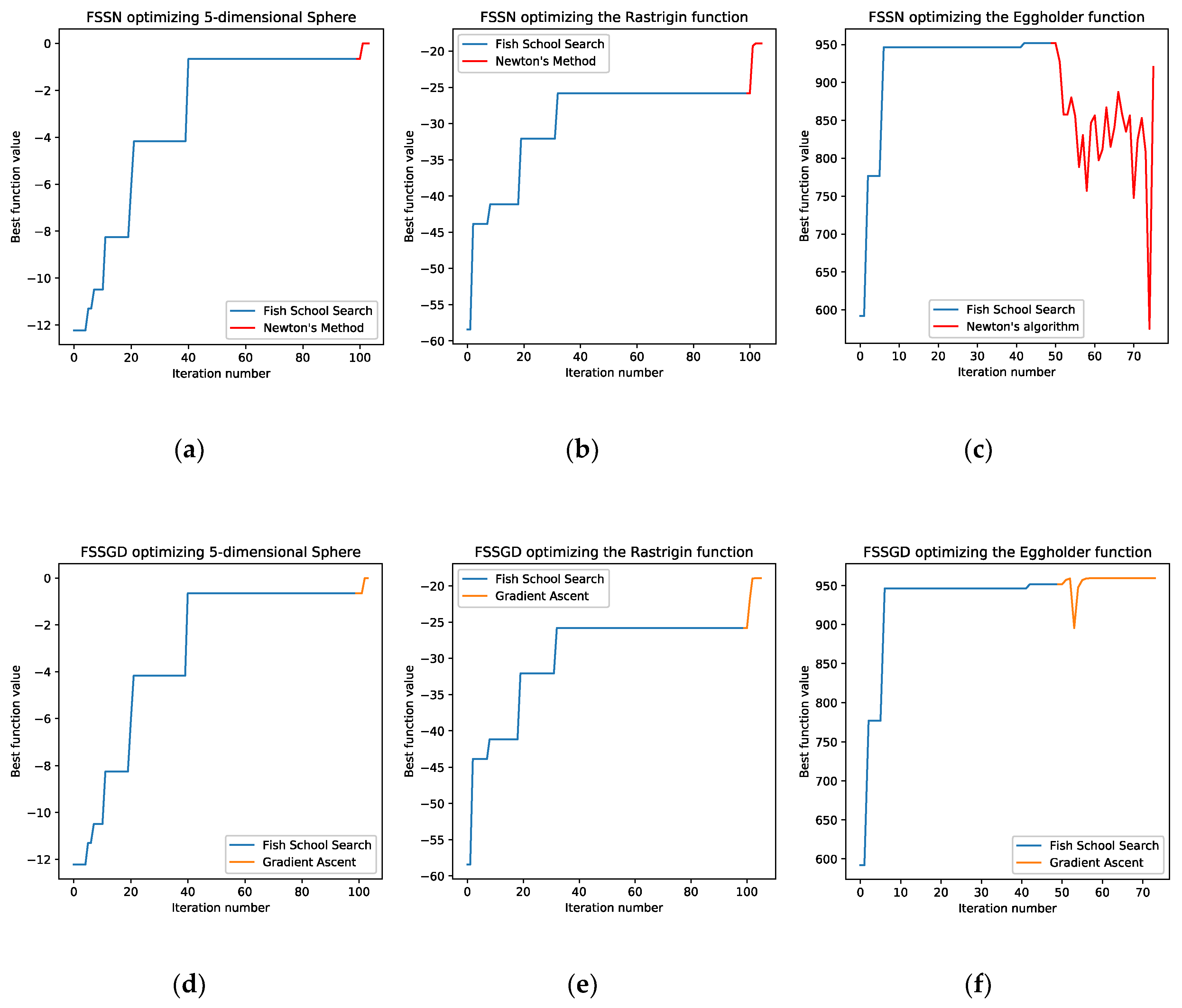
Each of the test functions listed in Table 1 was evaluated 50 times to determine how accurate the algorithms are, compared to each other. We gathered such metrics, as the best function value, mean function value, variance and standard deviation. Here, the best value denotes the closest value to the optimum of the considered fitness function. The results are shown in Table 2 and in Table 3, where the best result in each row is highlighted in bold. We use the FSSN abbreviation for the hybrid algorithm, which is based on fish school search and Newton’s optimization method. The FSSGD abbreviation denotes the hybrid algorithm where gradient ascent is used. Benchmark results for two-dimensional, three-dimensional and ten-dimensional versions of multidimensional functions and were deliberately omitted for brevity. The omitted results are similar to those shown in Table 2 and in Table 3.
From the obtained results, shown in Table 2 and in Table 3, we see that the hybrid algorithms generally perform better than the original algorithm. To demonstrate the convergence process of the hybrid algorithms, we obtained the plots shown in Figure 2.
As shown in Figure 2, the classical algorithms can either slightly improve the obtained solution, as shown in (a) and (d) plots, or considerably, as shown in (b) and (e) plots. The plots (c) and (f) show that the FSSN hybrid can diverge on multimodal optimization problems that can be solved fine by FSSGD. The FSSN hybrid algorithm based on Newton’s method diverges in a multimodal search space in the direction towards saddle points, local minima and local maxima. The hybrid based on the collective behavior of fish schools and gradient ascent successfully converged to the optimal solution.
The hybrid algorithm based on fish school search and Newton’s method in optimization can show accurate results, but has limited applications. For example, the Newton’s algorithm is not applicable to a function which Hessian matrix is singular, because a singular matrix is not invertible. Another limitation is the possible convergence to a wrong solution when optimizing a multimodal function. The method can converge, for example, to a saddle point. The use of the hybrid algorithm based on the collective behavior of fish schools and gradient ascent does not impose such limitations. This hybrid algorithm can be used in cases, when a function is differentiable inside the study region, by computing the derivative either numerically, by using finite difference approximations, or symbolically.
Additionally, we benchmarked the time required for the original and hybrid algorithms to optimize the functions listed in Table 1. The results are shown in Table 4 and Table 5, where the best result in each row is highlighted in bold.
From Table 4 and Table 5 we can conclude that the hybrid algorithms usually run a bit longer than the evolutionary-inspired algorithm without modifications. However, according to Table 2 and Table 3, in most cases the hybrids find solutions that are more accurate. The FSSGD algorithm is generally faster than the FSSN algorithm. The cause of this is that the hybrid algorithm based on Newton’s method computes the Hessian matrix on each iteration, using finite difference approximation, and such computations can be expensive, especially in high-dimensional space.
To verify, that the hybrid algorithms outperform the original algorithm, we used the Wilcoxon signed-ranks statistical test, often used to determine if significant statistical differences exist between two algorithms in computational intelligence. The results are shown in Table 6.
In our case, we ensured that the significant differences exist between FSS and FSSN, and between FSS and FSSGD. We assumed the level of significance , which means the 95% confidence level. The null hypothesis is that the two related paired samples come from the same distribution. For each test function listed in Table 1, we ran the original algorithm and hybrids 20 times. Then, we applied the Wilcoxon signed-ranks statistical test to the obtained distributions of solutions.
Based on the results shown in Table 6, we observed, that both of the hybrid algorithms can improve the accuracy of the original population-based algorithm, and in most cases, a statistically significant difference exists between the distributions the considered algorithms produce. The FSSN hybrid, which is based on Newton’s optimization method, outperforms the FSSGD hybrid based on gradient ascent, however in some cases Newton’s method converges to a stationary point or is not applicable to a function due to the singularity of its Hessian matrix in the given point. The FSSGD hybrid based on gradient ascent is more stable and shows more accurate results, than the original FSS algorithm; and can be used in cases, when the fitness function is differentiable in the study region.
4. Solution for the Linearly Inseparable XOR Problem
A neural network can be described as a programmatic system which allows making decisions using the evolution of a complex non-linear system. Such decisions are based on recognized underlying relationships in datasets. Neural networks take in a vector encoding the input object; the output signal of a neural network encodes the decision made by the system [38]. A perceptron is a mathematical model, proposed by Frank Rosenblatt in 1957; it can be treated as a simple neural network used to classify the data into two classes. Neural networks are often trained using back propagation, however, evolutionary algorithms show promising results as well [39,40,41]. As shown in [26], a hybrid algorithm which incorporates evolutionary-inspired and classical optimization techniques can achieve faster convergence speed and better accuracy.
The FSSGD, as the most effective hybrid algorithm proposed in this paper, can be used to optimize loss functions of neural networks, in cases, when the loss function of a perceptron is differentiable inside the study region. As a proof-of-concept, we used FSSGD as the loss function optimization algorithm to train a multi-layer perceptron. We were solving the linearly inseparable exclusive disjunction (XOR) problem [42], commonly used to benchmark neural network optimization algorithms [43]. In the problem we consider, we have the set of input objects, and the set of answers. Both the objects and the answers are Boolean values, belonging to the set. The goal is to restore the function using a multi-layer perceptron. The binary XOR function can be described by Table 7.
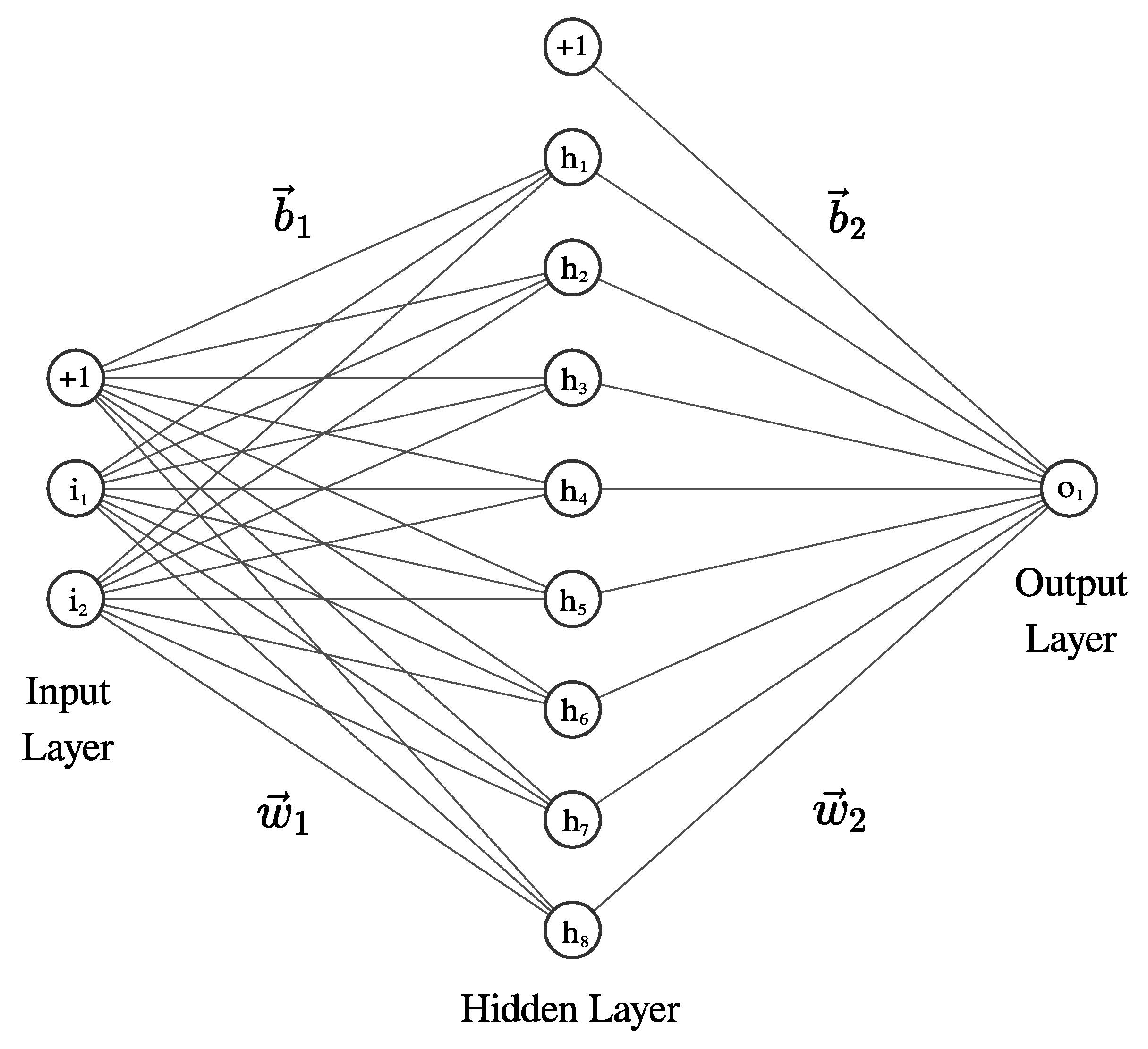
To solve the formulated problem, we built a perceptron with one hidden layer consisting of eight neurons. Other neural network architectures exist, which can solve the XOR problem [43,44], but the goal of the experiment was to see how the FSSGD algorithm would deal with a plenty of conflicting solutions. Perceptron architecture is shown in Figure 3.
On the hidden layer, we used the hyperbolic tangent activation function, given by:
where, is the input signal multiplied by the weight value of a neuron. While the set of decisions of our neural network should be represented as the Boolean values, we used the sigmoid activation function on the output layer. The sigmoid activation function is given by:
We used the binary cross-entropy as the loss function for the multi-layer perceptron:
where, and are the set of objects and the set of answers, respectively; denotes the weights; is the -th answer ; is the -th object, ;
The training process of a neural network leads to the optimization of its loss function. In our case, we optimized the Equation (12) loss function, using the hybrid FSSGD algorithm, in respect to the weights vector . After the neural network loss function was optimized, we plotted the surface of the loss function using the method [45], which allows visualizing functions that live in very high-dimensional spaces. In this approach, one chooses two orthogonal direction vectors and . The loss function is transformed into the following function parameterized by two arguments:
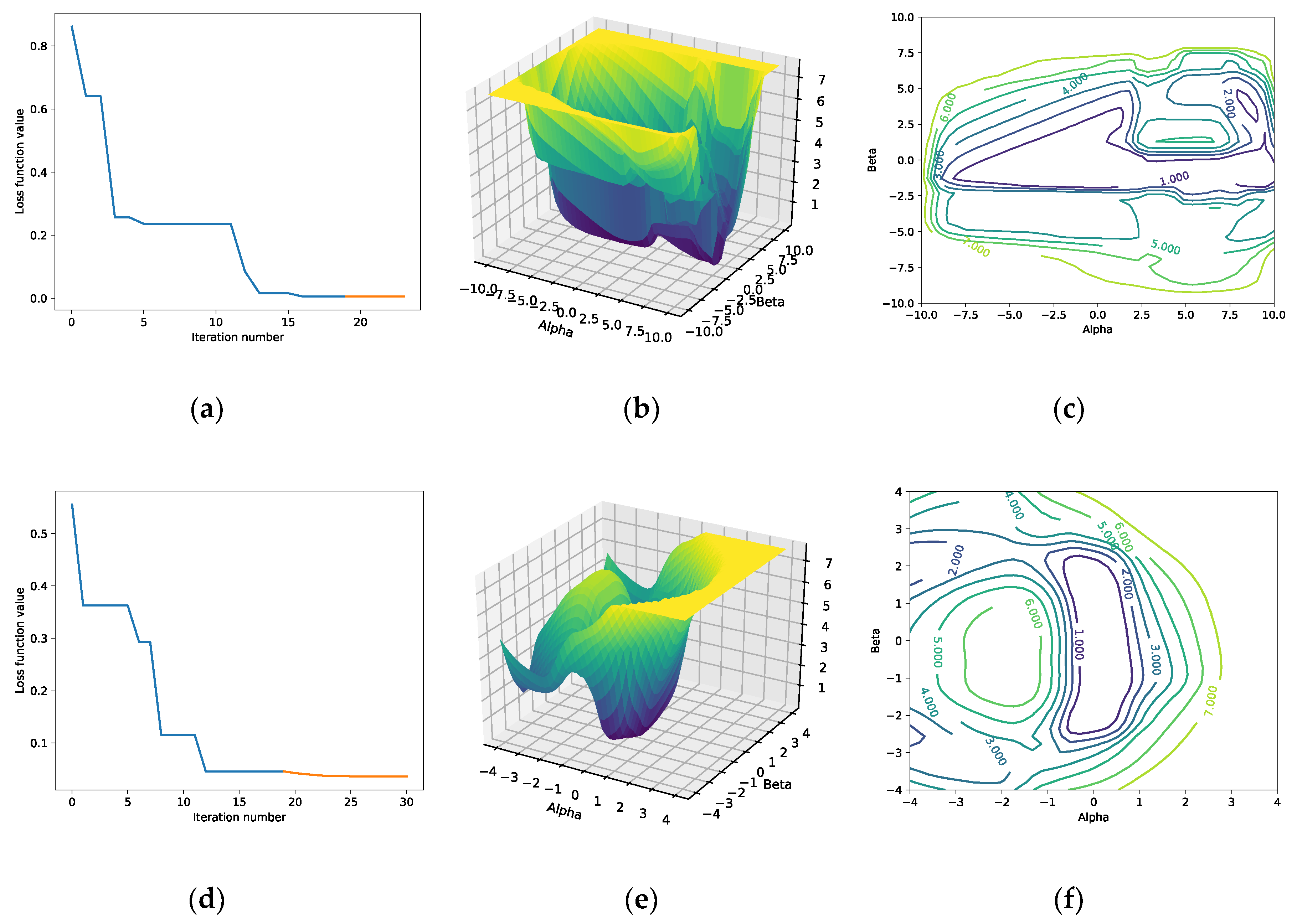
where, and are the objects and answers, respectively, is the optimized weights vector, and are the scalar coefficients required to visualize the function in the three-dimensional space. The loss function was optimized twice, using different parameter sets of the hybrid algorithm. The obtained results are shown in Figure 4.
In the first run, we defined the parameters as the variable denotes that coordinate components of each agent are bounded inside the region In the second case, the parameters were defined as , other parameters were left the same.
When using , it took 22 iterations for FSSGD to converge. When using , it took 30 iterations for the hybrid to converge. When using , the neural network output is more accurate, compared to the results obtained when . The same pseudorandom number generator seed was used in both experiments. Assuming the fact, that the obtained solutions differ, we can suppose, that if we increase the value, then we can get other, probably better, solutions. Notably, in Figure 4b,c,e,f, we see that the surface of the neural network loss function has a plenty of local minima points that can prevent the classical optimization algorithms from finding the global optimum. In Figure 4d we see, how finite difference-based gradient descent improves the solution obtained using Fish School Search.
5. Neural Network Hyperparameter Optimization
Modern neural networks achieve excellent performance in a wide variety of fields, but accuracy of predictions made by a neural network highly depends on chosen hyperparameters. The hyperparameters are the parameters usually adjusted by a researcher; such parameters include layer count in a neural network, neuron count on each layer, optimizer and learning rate, activation functions. Evolutionary-inspired algorithms are commonly used for neural network architecture optimization; neural network topologies can be evolved, for example, by using genetic algorithms [46] or particle swarm algorithms [47]. Training neural networks takes time, especially in deep learning. The benefit of using population-based algorithms is that such algorithms can be distributed across different worker nodes easily, and that can drastically reduce the amount of time required to run a single iteration of an optimization algorithm.
We applied the FSSGD algorithm to neural network hyperparameter optimization, evolving the architecture of a neural network for the prediction of house prices. Different neural networks were trained on the well-known Boston Housing dataset [48]. The Boston Housing dataset is relatively small, consisting of 506 rows and 14 columns. Each column represents the factor, which can potentially affect the price of a house. The dataset is split into training and testing data frames, the former consisted of 404 rows, and the latter consisted of 102 rows. We applied the feature normalization technique to the dataset by subtracting the mean value from the data and diving the data by standard deviation.
Each of the considered neural network architectures consisted of two layers. The optimized parameters were defined as follows: denoted neuron count on the first layer, ; denoted neuron count on the second layer, ; denoted the activation function used on the first layer, ; denoted the activation function used on the second layer, ; denoted the learning rate; denoted the optimizer used to train the neural network, . Neural network models were built with Keras and Tensorflow libraries. During every call to the fitness function of FSSGD, a parameterized model was trained during 50 epochs. The k-fold cross-validation technique was used to obtain the score of the model, assuming . During the training process of different neural networks, the mean squared error loss function was used:
Assuming and are the sets of objects and answers, respectively, is the -th object, ; is the -th answer, ; denotes the predictions generated by the neural network; . Due to the use of the k-fold cross-validation technique, the training dataset was split into three data frames, then two of the three data frames were used to train the neural network; the one data frame left was used to test the network. During the training phase, the value was set equal to 270; during the testing phase, the value was set to 134. The mean absolute error function was used to estimate the fitness score of the model:
The reason for using the mean absolute error metric seen in Equation (15) is that it produces results that can be easily interpreted by a human. In the Boston Housing dataset, we were solving a linear regression problem to predict house prices, so the mean absolute error metric gives us the error value in thousands of dollars.
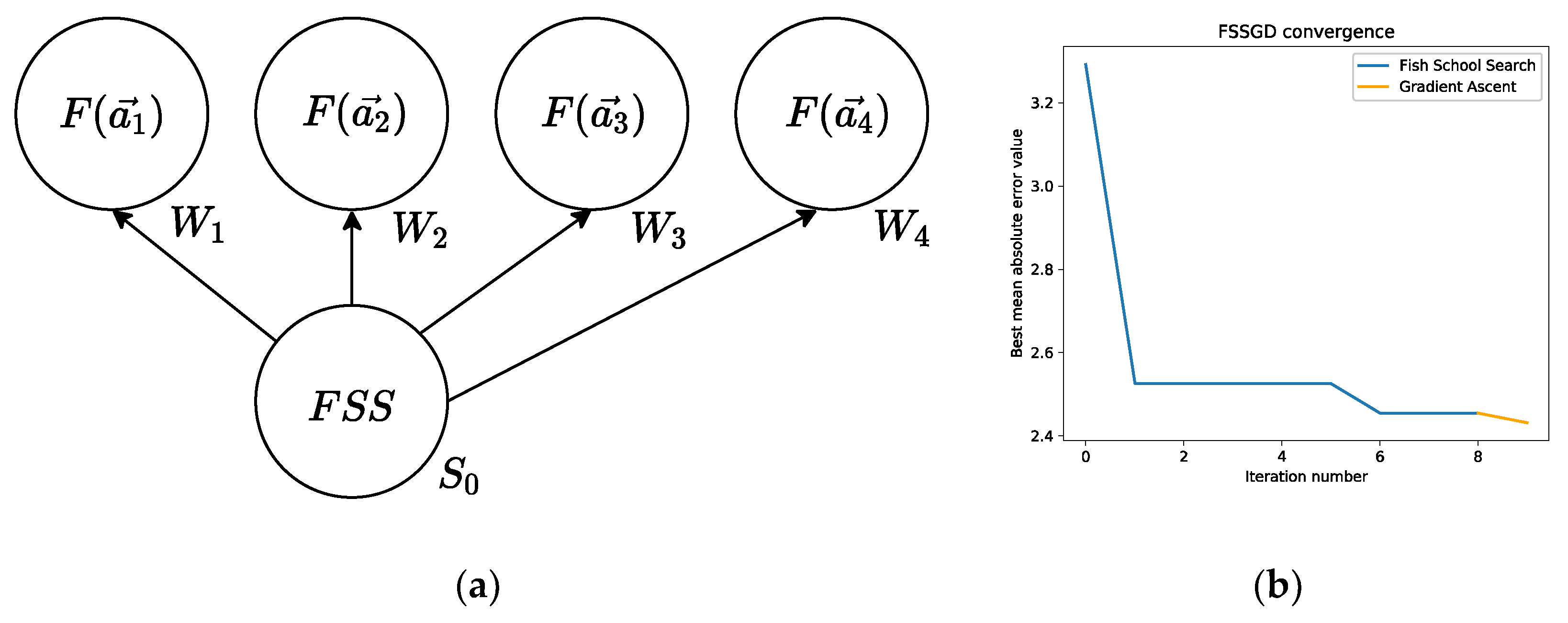
To handle the experiment, five Ubuntu 18.04 LTS nodes were rented on Microsoft Azure. For the FSS part of the proposed FSSGD algorithm, four agents were spawned. The FSS algorithm was running on the server node; fitness function values were computed on each iteration of the algorithm, the computations were distributed across four worker nodes. For the FSS part of the hybrid algorithm, we assumed On each fitness function call, separate neural network models were built and trained on different worker nodes multiple times, using k-fold cross-validation, to estimate the quality of a model according to Equation (15). The distributed computations architecture of the FSS algorithm is illustrated in Figure 5a.
For the gradient descent part of the FSSGD hybrid algorithm, we used finite difference approximation to compute first-order partial derivatives for the gradient vector numerically on each iteration; the computations were distributed across four worker nodes as well, assuming ; negative and positive derivative values were rounded down and up, respectively. Each worker node computed its own first-order partial derivative. The convergence of the hybrid algorithm optimizing neural network architecture is shown in Figure 5b.
The first layer of the evolved neural network model consisted of 58 neurons; the second layer consisted of 78 neurons; the softmax and tanh activation functions were used on the first and second layers, respectively. The optimizer selected by FSSGD was RMSprop with learning rate. The mean absolute error Equation (15) metric value obtained on the testing data frame was equal to 2.43, this is equivalent to 2430 USA dollars. The minimum price of a house in the Boston Housing dataset is 5000, the maximum price equals to 50,000 USA dollars. It took 1097 seconds total for the FSSGD algorithm to optimize the architecture in distributed mode, using four worker nodes, as shown in Figure 5a; 560 seconds for 8 iterations of FSS and 537 seconds for 2 iterations of gradient descent; the gradient descent computations were based on finite difference approximation of the fitness function. Without using the distributed approach to fitness function computations, it took more than an hour for the hybrid algorithm to converge.
The obtained results confirm that the hybrid algorithm based on the collective behavior of fish schools and gradient descent can produce slightly more accurate results, than the original population-based algorithm. However, when optimizing hyperparameters of neural networks the time losses required to compute the gradient vector numerically are too big, due to a large number of fitness function calls required to obtain the vector consisting of first-order partial derivatives, even in case if computations are distributed across multiple nodes. With the increase of search space dimensionality, the time required to compute the gradient of a fitness function increases, and this makes this technique not suitable for hyperparameter optimization of deep neural networks.
6. Discussion
The benchmarks of the proposed FSSN and FSSGD hybrid algorithms, which are based on the collective behavior of fish schools and classical optimization methods, on test functions for optimization, including the multidimensional Rastrigin, Rosenbrock, Sphere, Ackley, Michalewicz, Eggholder, Styblinsky–Tang function and others, indicate, that the hybrid algorithms generally produce more accurate solutions, and the Wilcoxon signed-rank test confirms that. The improvement in accuracy costs minor time losses, but the time losses increase with the increase of search space dimensionality.
The FSSN algorithm imposes a number of limitations upon the optimized function and has a chance to converge to the nearest saddle point, or to the wrong extremum. The FSSN algorithm can often produce solutions that are more accurate compared to FSS or FSSGD. However, the computations of the Hessian matrix can be quite expensive, especially in high-dimensional search space, or in cases, when the evaluation of a fitness function takes a long time to complete. In addition, there are such cases, when the Hessian matrix of the optimized function becomes singular. The Newton’s optimization method requires the Hessian matrix to be invertible, so in case if the matrix is singular, the method is unable to proceed with the optimization process. The FSSGD algorithm only requires the fitness function to be differentiable inside the study region. Gradient vector computations using finite difference approximation are far less expensive than Hessian matrix computations, so the time losses introduced by performing local search by gradient ascent are quite small, as shown in Table 4 and in Table 5. Except from using numerical differentiation, the gradient of a fitness function can be obtained by either using symbolical or automatic differentiation, and in this case, the time losses become even smaller.
The proposed FSSGD algorithm can be applied to such practical tasks, as optimization of loss functions in neural networks or SVM classifiers. When training neural networks, the full gradient descent method can be replaced with its modifications, commonly used to train neural networks, to speed up the optimization process.
The FSSGD algorithm can be applied to hyperparameter tuning of a neural network as well, but in this case, the time losses become unaffordable due to the fact, that the derivative of a fitness function cannot be found analytically or symbolically here. The only option left is numerical differentiation, which takes a large amount of time, especially in high-dimensional spaces and in cases, when the fitness function is either computationally expensive or takes a long time to execute due to other reasons. Hence, for neural network hyperparameter optimization it is better to use the original evolutionary-inspired FSS algorithm. In evolutionary-inspired algorithms, fitness function computations can be easily distributed across different worker nodes, and this can considerably speed up the optimization process.
Future research could compare various hybrid algorithms based on FSS and Quasi-Newton methods. Notably, a hybrid algorithm based on particle swarm optimization and the Broyden–Fletcher–Goldfarb–Shanno optimization method showed a strong advantage in [28]. Considering loss function optimization in neural networks, future work could compare the proposed FSSGD algorithm with other gradient-based methods, commonly used to train neural networks, such as Adam or stochastic gradient descent with momentum [49]. Another promising research area is chaos theory in evolutionary optimization. The initial locations of agents in swarm intelligence algorithms affect the quality of the obtained solution, so a chaos-based pseudorandom number generator could be used to initialize the population in an evolutionary-inspired algorithm [50].
Author Contributions
Conceptualization, guidance, supervision, validation, L.A.D.; software, resources, visualization, testing, A.V.G.; original draft preparation, L.A.D. and A.V.G. All authors have read and agreed to the published version of the manuscript.
Funding
This research received no external funding.
Conflicts of Interest
The authors declare no conflict of interest.
References
- Cagnina, L.; Esquivel, S.; Coello, C. Solving Engineering Optimization Problems with the Simple Constrained Particle Swarm Optimizer. Informatica 2008, 32, 319–326. [Google Scholar]
- Korneev, A.; Sukhanov, A. Investigation of accuracy and speed of convergence of algorithms of stochastic optimization of functions on a multidimensional space. Vestn. Astrakhan State Tech. Univ. Ser. Manag. Comput. Sci. Inform. 2018, 3, 26–37. (In Russian) [Google Scholar] [CrossRef]
- Ponsich, A.; Jaimes, A.L.; Coello, C.A.C. A Survey on Multiobjective Evolutionary Algorithms for the Solution of the Portfolio Optimization Problem and Other Finance and Economics Applications. IEEE Trans. Evol. Comput. 2013, 17, 321–344. [Google Scholar] [CrossRef]
- Demidova, L.; Gorchakov, A. The research and development of the hybrid algorithm based on the collective behavior of Fish schools and the classical optimization methods. IOP Conf. Ser. Mater. Sci. Eng. 2020, 734, 012090. [Google Scholar] [CrossRef]
- Li, Y.; Wu, H. A Clustering Method Based on K-Means Algorithm. Phys. Procedia 2012, 25, 1104–1109. [Google Scholar] [CrossRef] [Green Version]
- Goodman, E. Introduction to Genetic Algorithms. In Proceedings of the Genetic and Evolutionary Computation Conference, GECCO, London, UK, 7–11 July 2007; pp. 3205–3224. [Google Scholar]
- Shi, Y.; Eberhart, R. A Modified Particle Swarm Optimizer. In Proceedings of the IEEE International Conference on Evolutionary Computation, Anchorage, AK, USA, 4–9 May 1998; pp. 69–73. [Google Scholar]
- Dorigo, M.; Birattari, M.; Stützle, T. Ant Colony Optimization. IEEE Comput. Intell. Mag. 2006, 1, 28–39. [Google Scholar] [CrossRef]
- Reza, A.; Mohammadi, S.; Ziarati, K. A novel bee swarm optimization algorithm for numerical function optimization. Commun. Nonlinear Sci. Numer. Simul. 2010, 15, 3142–3155. [Google Scholar]
- Bastos Filho, C.; Lima Neto, F.; Lins, A.; Nascimento, A.; Lima, M. A Novel Search Algorithm based on Fish School Behavior. In Proceedings of the 2008 IEEE International Conference on Systems, Man and Cybernetics, Singapore, 12–15 October 2008; pp. 2646–2651. [Google Scholar]
- Chehouri, A.; Younes, R.; Khoder, J.; Perron, J.; Ilinca, A. A Selection Process for Genetic Algorithm Using Clustering Analysis. Algorithms 2017, 10, 123. [Google Scholar] [CrossRef] [Green Version]
- Demidova, L.; Nikulchev, E.; Sokolova, Y. Big Data Classification Using the SVM Classifiers with the Modified Particle Swarm Optimization and the SVM Ensembles. Int. J. Adv. Comput. Sci. Appl. 2016, 7, 294–312. [Google Scholar] [CrossRef] [Green Version]
- Shah, S.; Pradhan, M. R-GA: An Efficient Method for Predictive Modelling of Medical Data Using a Combined Approach of Random Forests and Genetic Algorithm. ICTACT J. Soft Comput. 2016, 6, 1153–1156. [Google Scholar]
- Janati, I.; Mohammed, A.; Ramchoun, H.; Ghanou, Y.; Ettaouil, M. Genetic Algorithm for Neural Network Architecture Optimization. In Proceedings of the 2016 3rd International Conference on Logistics Operations Management (GOL), Fez, Morocco, 23–25 May 2016; pp. 1–4. [Google Scholar]
- Filho, J.B.M.; de Albuquerque, I.M.C.; de Lima Neto, F.B.; Ferreira, F.V.S. Optimizing Multi-plateau Functions with FSS-SAR (Stagnation Avoidance Routine). In Proceedings of the 2016 IEEE Symposium Series on Computational Intelligence, Athens, Greece, 6–9 December 2016; pp. 1–7. [Google Scholar]
- Bastos Filho, C.; Guimarães, A. Multi-Objective Fish School Search. Int. J. Swarm Intell. Res. 2017, 6, 23–40. [Google Scholar] [CrossRef]
- Roy, P.; Mahapatra, G.S.; Dey, K.N. Forecasting of software reliability using neighborhood fuzzy particle swarm optimization based novel neural network. IEEE/CAA J. Autom. Sin. 2019, 6, 1365–1383. [Google Scholar]
- Wang, L.; Lu, J. A memetic algorithm with competition for the capacitated green vehicle routing problem. IEEE/CAA J. Autom. Sin. 2019, 6, 516–526. [Google Scholar] [CrossRef]
- Gao, S.; Yu, Y.; Wang, Y.; Wang, J.; Cheng, J.; Zhou, M. Chaotic Local Search-Based Differential Evolution Algorithms for Optimization. IEEE Trans. Syst. Man Cybern. Syst. 2019, 99, 1–14. [Google Scholar] [CrossRef]
- Bastos Filho, C.; Nascimento, D.O. An Enhanced Fish School Search Algorithm. In Proceedings of the 1st BRICS Countries Congress on Computational Intelligence, BRICS-CCI, Recife, Brazil, 8–11 September 2013; pp. 152–157. [Google Scholar]
- Dos Santos, W.; Barbosa, V.; Souza, R.; Ribeiro, R.; Feitosa, A.; Silva, V.; Ribeiro, D.; Covello de Freitas, R.; Lima, M.; Soares, N.; et al. Image Reconstruction of Electrical Impedance Tomography Using Fish School Search and Differential Evolution. In Critical Developments and Applications of Swarm Intelligence; IGI Global: Hershey, PA, USA, 2018. [Google Scholar]
- Bova, V.; Kuliev, E.; Rodzin, S. Prediction in Intellectual Assistant Systems Based on Fish School Search Algorithm. Izv. Sfedu Eng. Sci. 2019, 2, 34–47. [Google Scholar]
- Carneiro de Albuquerque, I.M.; Monteiro Filho, J.; Lima Neto, F.; Silva, A. Solving Assembly Line Balancing Problems with Fish School Search algorithm. In Proceedings of the 2016 IEEE Symposium Series on Computational Intelligence (SSCI), Athens, Greece, 6–9 December 2016; pp. 1–8. [Google Scholar]
- Ananthi, J.; Ranganathan, V.; Sowmya, B. Structure Optimization Using Bee and Fish School Algorithm for Mobility Prediction. Middle-East J. Sci. Res. 2016, 24, 229–235. [Google Scholar]
- Requena-Perez, M.E.; Albero-Ortiz, A.; Monzo-Cabrera, J.; Diaz-Morcillo, A. Combined use of genetic algorithms and gradient descent methods for accurate inverse permittivity measurement. IEEE Trans. Microw. Theory Tech. 2006, 54, 615–624. [Google Scholar] [CrossRef]
- Ganjefar, S.; Tofighi, M. Training qubit neural network with hybrid genetic algorithm and gradient descent for indirect adaptive controller design. Eng. Appl. Artif. Intell. 2017, 65, 346–360. [Google Scholar] [CrossRef]
- Reddy, M.P.; Ganguli, R. An Automated Gradient Enhanced Bat Algorithm. In Proceedings of the 2018 IEEE Symposium Series on Computational Intelligence (SSCI), Bangalore, India, 18–21 November 2018; pp. 2353–2360. [Google Scholar]
- Dos Santos Coelho, L.; Mariani, V.C. Particle Swarm Optimization with Quasi-Newton Local Search for Solving Economic Dispatch Problem. In Proceedings of the 2006 IEEE International Conference on Systems, Man and Cybernetics, Taipei, Taiwan, 8–11 October 2006; pp. 3109–3113. [Google Scholar]
- Gong, Y.-J.; Chen, W.-N.; Zhan, Z.-H.; Zhang, J.; Li, Y.; Zhang, Q.; Li, J.-J. Distributed evolutionary algorithms and their models: A survey of the state-of-the-art. Appl. Soft Comput. 2015, 34, 286–300. [Google Scholar] [CrossRef] [Green Version]
- Polyak, B. Newton’s method and its use in optimization. Eur. J. Oper. Res. 2007, 181, 1086–1096. [Google Scholar] [CrossRef]
- McClarren, R. Finite Difference Derivative Approximations. In Computational Nuclear Engineering and Radiological Science Using Python; Academic Press: London, UK, 2018; pp. 251–266. [Google Scholar]
- Hussain, K.; Salleh, M.; Cheng, S.; Naseem, R. Common Benchmark Functions for Metaheuristic Evaluation: A Review. Int. J. Inform. Vis. 2017, 1, 218–223. [Google Scholar] [CrossRef]
- Mesa, E.; Velásquez, J.; Jaramillo, P. Evaluation and Implementation of Heuristic Algorithms for Non-Restricted Global Optimization. IEEE Lat. Am. Trans. 2015, 13, 1542–1549. [Google Scholar] [CrossRef]
- Rosenbrock, H. An automatic method for finding the greatest or least value of a function. Comput. J. 1960, 3, 175–184. [Google Scholar] [CrossRef] [Green Version]
- Mühlenbein, H.; Schomisch, D.; Born, J. The Parallel Genetic Algorithm as Function Optimizer. Parallel Comput. 1991, 17, 619–632. [Google Scholar] [CrossRef]
- Momin, J.; Xin-She, Y. A literature survey of benchmark functions for global optimization problems. Int. J. Math. Model. Numer. Optim. 2013, 4, 150–194. [Google Scholar]
- Odili, J.; Noraziah, A. African Buffalo Optimization for Global Optimization. Curr. Sci. 2018, 114, 627–636. [Google Scholar] [CrossRef]
- Sigov, A.; Andrianova, E.; Zhukov, D.; Zykov, S.; Tarasov, I. Quantum informatics: Overview of the main achievements. Russ. Technol. J. 2019, 7, 5–37. (In Russian) [Google Scholar] [CrossRef] [Green Version]
- Gao, S.; Zhou, M.; Wang, Y.; Cheng, J.; Yachi, H.; Wang, J. Dendritic Neuron Model With Effective Learning Algorithms for Classification, Approximation, and Prediction. IEEE Trans. Neural Netw. Learn. Syst. 2019, 30, 601–614. [Google Scholar] [CrossRef]
- Wang, J.; Kumbasar, T. Parameter optimization of interval Type-2 fuzzy neural networks based on PSO and BBBC methods. IEEE/CAA J. Autom. Sin. 2019, 6, 247–257. [Google Scholar] [CrossRef]
- Luo, Y.; Zhao, S.; Yang, D.; Zhang, H. A new robust adaptive neural network backstepping control for single machine infinite power system with TCSC. IEEE/CAA J. Autom. Sin. 2020, 7, 48–56. [Google Scholar] [CrossRef]
- Gruzling, N. Linear Separability of the Vertices of an n-Dimensional Hypercube. Master’s Thesis, University of Nothern British Columbia, Prince George, BC, Canada, 2001. [Google Scholar]
- Reljan-Delaney, M.; Wall, J. Solving the Linearly Inseparable XOR Problem with Spiking Neural Networks. In Proceedings of the 2017 SAI Computing Conference, London, UK, 18–20 July 2017; pp. 701–705. [Google Scholar]
- Piazza, F.; Uncini, A.; Zenobi, M. Artificial neural networks with adaptive polynomial activation function. Int. Jt. Conf. Neural Netw. 1992, 2, 343–348. [Google Scholar]
- Goodfellow, I.; Vinyals, O.; Saxe, A. Qualitatively Characterizing Neural Network Optimization Problems. In Proceedings of the 3rd International Conference on Learning Representations, ICLR 2015, San Diego, CA, USA, 7–9 May 2015. [Google Scholar]
- Stanley, K.O.; Miikkulainen, R. Evolving Neural Networks through Augmenting Topologies; MIT Press: Cambridge, MA, USA, 2002; pp. 99–127. [Google Scholar]
- Carvalho, M.; Ludermir, T. Particle Swarm Optimization of Neural Network Architectures and Weights. In Proceedings of the 7th International Conference on Hybrid Intelligent Systems, HIS 2007, Kaiserlautern, Germany, 17–19 September 2007; pp. 336–339. [Google Scholar]
- Harrison, D.; Rubinfeld, D.L. Hedonic prices and the demand for clean air. J. Environ. Econ. Manag. 1978, 5, 81–102. [Google Scholar] [CrossRef] [Green Version]
- Ruder, S. An Overview of Gradient Descent Optimization Algorithms. 2017. Available online: https://arxiv.org/pdf/1609.04747.pdf (accessed on 10 March 2020).
- Ma, Z.; Yuan, X.; Han, S.; Sun, D.; Ma, Y. Improved Chaotic Particle Swarm Optimization Algorithm with More Symmetric Distribution for Numerical Function Optimization. Symmetry 2019, 11, 876. [Google Scholar] [CrossRef] [Green Version]
Figure 1.
(a) Dual Eggholder function search area, which has many local extreme points. (b) A fish school optimizing the dual two-dimensional Styblinsky–Tang function .
Figure 1.
(a) Dual Eggholder function search area, which has many local extreme points. (b) A fish school optimizing the dual two-dimensional Styblinsky–Tang function .

Figure 2.
Hybrid algorithms optimizing test functions from Table 1.
Figure 2.
Hybrid algorithms optimizing test functions from Table 1.

Figure 3.
Perceptron built to benchmark the FSSGD algorithm; eight neurons were used to increase the number of possible conflicting solutions. The and vectors denote the weights of the connections between the input and hidden layers and between the hidden and output layers, respectively; and are the biases. The biases have the same dimensions as their output vectors. denote the neurons of the input, hidden and output layers respectively.

Figure 4.
(a) FSSGD algorithm convergence when ; (b) loss function surface visualization near the suboptimal solution, ; (c) contour plot of the loss function, . (d) FSSGD algorithm convergence when ; (e) loss function surface visualization near the suboptimal solution, ; (f) Contour plot of the loss function, .

Figure 5.
(a) Network topology for the distributed version of the FSS algorithm. Here, denotes the -th agent; is the time-consuming fitness function; is the -th worker; is the server, which hosts the algorithm; (b) FSSGD algorithm convergence when optimizing hyperparameters.
Figure 5.
(a) Network topology for the distributed version of the FSS algorithm. Here, denotes the -th agent; is the time-consuming fitness function; is the -th worker; is the server, which hosts the algorithm; (b) FSSGD algorithm convergence when optimizing hyperparameters.


Table 1.
Test functions used to benchmark the hybrid optimization algorithms.
| Test Function Formula | Dimension | Search Area | Optimum |
|---|---|---|---|
| 3, 5, 10 | |||
| 3, 5, 10 | |||
| 3, 5, 10 | |||
| 3, 5, 10 | |||
| 2 | |||
| 2 | |||
| 2 | |||
| 2 | |||
| 2, 5, 10 |
Table 2.
Accuracy comparison of the algorithms optimizing 5-dimensional functions from Table 1.
Table 2.
Accuracy comparison of the algorithms optimizing 5-dimensional functions from Table 1.
| Function | Metric | FSS | FSSN | FSSGD |
|---|---|---|---|---|
| Mean | ||||
| Best | ||||
| Std. dev | ||||
| Mean | ||||
| Best | ||||
| Std. dev | ||||
| Mean | ||||
| Best | ||||
| Std. dev | ||||
| Mean | ||||
| Best | 0.00 | 0.00 | ||
| Std. dev | ||||
| Mean | ||||
| Best | ||||
| Std. dev |
Table 3.
Accuracy comparison of the algorithms optimizing 2-dimensional functions from Table 1.
Table 3.
Accuracy comparison of the algorithms optimizing 2-dimensional functions from Table 1.
| Function | Metric | FSS | FSSN | FSSGD |
|---|---|---|---|---|
| Mean | ||||
| Best | ||||
| Std. dev | ||||
| Mean | ||||
| Best | ||||
| Std. dev | ||||
| Mean | 951.06 | 951.57 | ||
| Best | ||||
| Std. dev | ||||
| Mean | ||||
| Best | ||||
| Std. dev |
Table 4.
Time benchmarks of 5-dimensional test functions listed in Table 1.
Table 4.
Time benchmarks of 5-dimensional test functions listed in Table 1.
| Function | Metric | FSS | FSSN | FSSGD |
|---|---|---|---|---|
| Mean | ||||
| Min | ||||
| Std. dev | ||||
| Mean | ||||
| Min | ||||
| Std. dev | ||||
| Mean | ||||
| Min | ||||
| Std. dev | ||||
| Mean | ||||
| Min | ||||
| Std. dev | ||||
| Mean | ||||
| Min | ||||
| Std. dev |
Table 5.
Time benchmarks of 2-dimensional test functions listed in Table 1.
Table 5.
Time benchmarks of 2-dimensional test functions listed in Table 1.
| Function | Metric | FSS | FSSN | FSSGD |
|---|---|---|---|---|
| Mean | ||||
| Min | ||||
| Std. dev | ||||
| Mean | ||||
| Min | ||||
| Std. dev | ||||
| Mean | 1.05 | |||
| Min | 1.03 | |||
| Std. dev | 0.01 | 0.01 | 0.01 | |
| Mean | ||||
| Min | ||||
| Std. dev |
Table 6.
Wilcoxon signed-rank test applied to the original and hybrid algorithms accuracy measurements. The sign of denotes whether FSSN algorithm outperforms Fish School Search (FSS), the sign of denotes whether FSSGD outperforms FSS, sign denotes whether FSSN outperforms FSSGD. The equality sign indicates no significant difference.
| Function | |||
|---|---|---|---|
Table 7.
Exclusive disjunction (XOR) function truth table.
| 0 | 0 | 0 |
| 0 | 1 | 1 |
| 1 | 0 | 1 |
| 1 | 1 | 0 |
© 2020 by the authors. Licensee MDPI, Basel, Switzerland. This article is an open access article distributed under the terms and conditions of the Creative Commons Attribution (CC BY) license (http://creativecommons.org/licenses/by/4.0/).
Share and Cite
MDPI and ACS Style
Demidova, L.A.; Gorchakov, A.V. Research and Study of the Hybrid Algorithms Based on the Collective Behavior of Fish Schools and Classical Optimization Methods. Algorithms 2020, 13, 85. https://0-doi-org.brum.beds.ac.uk/10.3390/a13040085
AMA Style
Demidova LA, Gorchakov AV. Research and Study of the Hybrid Algorithms Based on the Collective Behavior of Fish Schools and Classical Optimization Methods. Algorithms. 2020; 13(4):85. https://0-doi-org.brum.beds.ac.uk/10.3390/a13040085
Chicago/Turabian StyleDemidova, Liliya A., and Artyom V. Gorchakov. 2020. "Research and Study of the Hybrid Algorithms Based on the Collective Behavior of Fish Schools and Classical Optimization Methods" Algorithms 13, no. 4: 85. https://0-doi-org.brum.beds.ac.uk/10.3390/a13040085
Note that from the first issue of 2016, this journal uses article numbers instead of page numbers. See further details here.