Moving Deep Learning to the Edge


1
Instituto de Engenharia de Sistemas e Computadores-Investigação e Desenvolvimento (INESC-ID), Instituto Superior de Engenharia de Lisboa, Instituto Politécnico de Lisboa, 1959-007 Lisbon, Portugal
2
Instituto de Engenharia de Sistemas e Computadores-Investigação e Desenvolvimento (INESC-ID), Instituto Superior Técnico, Universidade de Lisboa, 1049-001 Lisbon, Portugal
*
Author to whom correspondence should be addressed.
Algorithms 2020, 13(5), 125; https://0-doi-org.brum.beds.ac.uk/10.3390/a13050125
Submission received: 29 March 2020
/
Revised: 16 May 2020
/
Accepted: 16 May 2020
/
Published: 18 May 2020
(This article belongs to the Section Evolutionary Algorithms and Machine Learning)
Abstract
:Deep learning is now present in a wide range of services and applications, replacing and complementing other machine learning algorithms. Performing training and inference of deep neural networks using the cloud computing model is not viable for applications where low latency is required. Furthermore, the rapid proliferation of the Internet of Things will generate a large volume of data to be processed, which will soon overload the capacity of cloud servers. One solution is to process the data at the edge devices themselves, in order to alleviate cloud server workloads and improve latency. However, edge devices are less powerful than cloud servers, and many are subject to energy constraints. Hence, new resource and energy-oriented deep learning models are required, as well as new computing platforms. This paper reviews the main research directions for edge computing deep learning algorithms.
1. Introduction
Over the last thirty years, Deep Learning (DL) algorithms have evolved very fast and have become promising algorithms with better results than other previous machine learning approaches [1]. Nonetheless, DL depends on the availability of high-performance computing platforms with a large amount of storage, required for the data needed to train these models [2]. Cloud computing has been the preferred computing model for running machine learning models, using data centers where a huge amount of processing power and storage is available [3,4].
However, the exponential increase of data traffic and low-latency requirements of many deep learning services are challenging this centralized computing model to guarantee the required quality of service [5]. The high bandwidth demanded of the communication networks to move such a volume of data is another important problem. Recent studies [6] report that by 2030, there will be an estimated 50 billion Internet of Things (IoT) connected devices. The traffic generated by all these devices will be close to 850 Zettabytes (ZB) by 2021, exceeding forty times the traffic generated in data centers [7].
Sending all these data to a central cloud to be processed has many problems. Cloud centers will soon exhaust the capacity to process such a massive amounts of data, and the communication networks will soon exhaust the available bandwidth [8,9]. Many DL applications have latency constraints, which, when not fulfilled, may have catastrophic consequences like, for example, autonomous driving [10]. Additionally, security and privacy matters are important when dealing with user data in a myriad of applications. Applications associated with smart cities and smart homes are a classical illustration of the need for privacy and security [11].
These limitations lead to the adoption of the edge computing paradigm [12], that is running DL near the edge, close to the source of the data [13]. Edge computing is a distributed computing paradigm that brings computing resources, memory, and services close to where the data are produced. This is a way to speed up responses and reduce dependencies on the availability of communication bandwidth.
A clear definition of the boundaries of the edge computing infrastructure does not exist. For most, the edge is a layer between the cloud and the user, where by “user”, it is meant a device or a container of several users [14]. In this paper, the edge layer is assumed to include all processing, storage, and networks surrounding the end device itself. At the edge, there may be several layers of processing and storage, including the device, customer premises, and edge servers. In this context, edge devices include end devices and edge nodes. End devices include all mobile devices, gadgets, and wearables that collect data and are closest to the user. Edge nodes include routers, switches, base stations, servers, cloudlets, microdata centers, and all kinds of servers deployed at the edge.
Several applications already benefit from using services and applications running on the edge. These applications can considerably be improved with DL algorithms, which determines the urgent necessity to be able to run these algorithms at the edge. Examples include:
- Smart cities: DL algorithms help improve the data traffic management, the privacy of city data, the local management, and the speed of response of smart city services [15];
- Smart homes: home living improvement to help people with personal data analysis and adaptation of services to different personal behaviors. Once again, personal data privacy is important and requires data processing services closer to the user [16];
- Automated driving: Self-driving vehicles like cars and drones require a real-time response and highly accurate object classification and recognition algorithms. High-performance edge computing, including DL algorithms, is necessary to guarantee accuracy and real-time response for self-driving vehicles [10];
- Industrial applications: accurate DL algorithms are needed to detect failures in production lines, foment automation in industrial production, and improve industrial management. These workloads must also be processed locally and in real-time [17].
Distributed computing platforms for edge computing will alleviate the computing and storage pressure on the cloud and make it easier to guarantee performance constraints [18]. These two computing paradigms differ in many aspects (see Table 1). They are not mutually exclusive, but, instead, must collaborate with each other to provide reliable high performance and storage requirements [19].
Edge computing is a paradigm already applied in many areas and services [20] and has recently been considered a candidate for running DL models [21]. While a good idea, this new DL service requires high computational and memory resources, which is a problem. Edge servers and end devices have much less computing and memory resources compared to a cloud data center [22]. Several research directions have been followed to overcome these limitations: (1) new architectures for edge servers integrated with cloud servers for an efficient computational coordination [23]; (2) new DL models with computing, memory, and energy concerns; (3) new hardware-oriented optimizations to improve performance and energy efficiency; (4) and new computing architectures oriented toward DL models. This article provides an overview and review of the approaches proposed in each of these research dimensions.
Previous reviews on the same subject have focused on the deployment of DL methods, such as Deep Neural Networks (DNN), into edge computing, with an emphasis on how the edge infrastructure is used for inference and training [13,18,24]. Others focus on hardware architectures for running DNNs [25]. This paper stresses the importance of considering simultaneously all four dimensions (edge computing architecture, model design, model optimization, and hardware accelerators) for the efficient design of DL edge solutions for edge nodes and end devices. The present review focuses on the migration of DL from the cloud to the very end devices, the final layer of edge computing. It highlights the increasing importance of the end device for an integrated DL solution, which clears the way for new user applications.
The paper is organized as follows. Section 2 introduces the methodology employed to do the review. Section 3 describes the fundamentals and the state-of-the-art on deep learning. Section 4 describes the methods and architectures being used to execute deep learning inference at the edge. Section 5 describes the methods and architectures proposed to train deep neural networks at the edge. Section 6 discusses the challenges and open issues about the deployment of deep learning at the edge. Section 7 concludes the paper.
2. Survey Methodology
In this review, the solutions proposed to deploy deep learning on the edge are identified and analyzed. Two questions are addressed: (1) Why deep learning should be executed on the edge and what applications can benefit from this? (2) How can this be achieved efficiently and effectively?
The survey described in this paper was elaborated in two steps. The first step was the collection of the bibliography associated with the topic. The second step consisted of the analysis and the review of this bibliography. The search for the bibliography about the design and deployment of deep learning on the edge was done using one main keyword and a list of secondary keywords. The search was carried out using several scientific databases like IEEE Xplore, ScienceDirect, Directory of Open Access Journals (DOAJ), and Scopus and web scientific indexing services, including Google Scholar and Web of Science.
The search focused on conference papers and journal articles published after 2015 since deep learning on the edge is a recent topic of research. However, some important works on deep learning are older than 2015. These works highly referenced in recent papers as fundamental for the development of deep learning were also included. Some technical reports of known global vendors were also included since these provide important data that justify some trends in the area of deep learning.
The main keyword used in the search was deep learning. This was followed by one or two keywords from a group of keywords associated with the organization of the paper: models, algorithms, application, mobile, edge, inference, training, hardware, device, processor, optimization, and architecture. Among all papers retrieved by the search process, the review considered only papers whose main topic was deep learning. These included papers that introduced advances in the design and development of deep learning models, algorithms, and architectures with emphasis on edge computing.
Even reducing the focus of deep learning to the edge, the review still has a broad spectrum of themes, and so, the volume of bibliographical references is enormous. To reduce this set to a manageable number, we considered the most cited and recent references whenever there were several references to the same sub-area. This permitted maintaining the flow of reading and considered many works referenced indirectly from the main references.
The articles collected were then analyzed to determine the evolution trend in the deployment of deep learning on the edge considering the following research directions
- Evolution of deep learning models from accuracy oriented to edge oriented;
- Application areas of deep learning when executed on the edge;
- Optimization of deep learning models to improve the inference and training;
- Computing devices to execute deep learning models on the edge;
- Edge computing solutions to run deep learning models;
- Methods to train deep learning models on the edge.
The evolution and trends of each of these research directions are reviewed and analyzed in the following sections.
3. Deep Learning
Deep learning [26] is a machine learning algorithm to teach computing systems to learn by example. Its computational complexity has delayed its deployment in a vast set of areas, including computer vision and language processing, among others [27]. Most deep learning-based approaches use deep neural networks, which are based on artificial neural networks.
An Artificial Neural Network (ANN) [28] is a computing model consisting of interconnected neurons organized in a stack of layers: an input layer to receive data to be processed, an output layer that provides the classification results of the network, and a set of hidden layers. Layers contain neurons that map all the inputs into an output to be used by the nodes of the next layer. The first ANN approaches had typically no more than three layers, in part because it was hard to train. Neural networks with more than three hidden layers are designated deep neural networks [29] to emphasize the high number of layers.
One of the first deep neural models was developed for handwritten classification [30]. Despite the high accuracy achieved, it was not largely accepted to replace other traditional machine learning algorithms because it was hard to train and implement. The better results of deep learning were not so evident because the application was not that difficult. Furthermore, its applicability to larger models was somehow limited by the computational capacity available at that time that was unable to train such large models in acceptable computing times. Only later [31], deep neural networks achieved popularity on solving several artificial intelligent tasks better than other machine learning algorithms.
Not only the computing platforms have improved considerably (e.g., Graphics Processing Units (GPU)), but also the training methods [32,33,34]. Both allowed the design of larger deep neural networks. The Internet has also contributed to the success of deep learning. The proliferation of the Internet has increased the availability of data required to train the networks with high accuracy.
The success of a deep neural network comes from the use of many hidden layers. One layer extracts hidden information from the input maps generated by the previous layer. Complex features are correlated as the data move forward through the sequence of layers [1,29]. The most common example of this behavior can be observed in an image classification task with a DNN. While the initial layers extract simple information about the image, the next layers correlate these simple objects to identify other more complex features. In the end, an image is associated with the class that has the closest set of complex features.
A neural network model is first trained to solve a particular problem and then used to classify new samples in a process known as inference. The training of the network determines its accuracy. Training a network can be supervised or unsupervised. In supervised training, the model learns from data manually labeled. The weights are adjusted so that the output of the network for a particular input matches the correct answer. Unsupervised training does not require labeled data. Instead, the model extracts patterns from the input by itself.
Supervised training is the process of finding the set of weights, W, that minimizes the error, E, between the measured outputs, , and the expected outputs, , for all input samples, . The error is determined with a loss function, E(W), as the sum of the squared error:
The training process iteratively runs forward propagation of input samples followed by backpropagation of the error. Starting with a random or a pre-trained set of weights, forward propagation applies an input to the network and determines its classification. The measured and the expected outputs are used by the loss function to determine the error between both.
The backpropagation than propagates backward the error found with the loss function; that is, outputs of neurons become inputs, and inputs become outputs. The weights of all neurons that contribute to the output are adjusted in proportion to their contribution to reducing the total loss. The adjustment of weights follows the gradient descent [35] technique:
where weights are incrementally updated proportionally to the derivative of the loss function. Even for simple models and problems, one-hundred percent accuracy is not achieved. The process is not guaranteed to find global minima, but converges to a minimum if iterated multiple times. To avoid excessive training times, training stops when the accuracy improvement is below a given threshold. A network can be trained without any initial knowledge or from an already-trained network where the initial weights are already close to the final values (fine-tuning).
While inference runs a forward propagation of the network only once, training is an iterative process that runs forward and backward propagation multiple times for multiple training input instances. Therefore, training is a more intensive computing task.
Different deep neural models are used for different classes of problems. Therefore, different deep learning models were proposed in the last few decades, and many different networks exist for each type. The Convolutional Neural Network (CNN) is one of the most applied deep learning models, followed by the Recurrent Neural Network (RNN), Long Short-Term Memory (LSTM), Restricted Boltzmann Machine (RBM), Deep Boltzmann Machine (DBM), Deep Belief Network (DBN), Auto-Encoder (AE), and several other models that are proposed every year.
The CNN is used for object classification and recognition in images and videos with a vast set of applications, like video surveillance. Therefore, it is the most studied deep neural network. One of the first deep neural networks proposed in [36] was a CNN for image classification. What differentiates a convolutional neural network from a traditional artificial neural network is the existence of convolutional layers. Convolutional layers take into consideration the correlation between neighbor pixels of the image and limit the connections between neurons of different layers to only those within a window of neighbor neurons. The convolution between a window of weights and the inputs of a neuron generates an activation sent to the neurons of the next layer. Each different kernel (stack of windows of weights) detects a particular feature of the image. Hence, a convolutional layer considers many different kernels. Features identified with the convolutional layers are fully correlated with dense layers. Known also as fully connected layers, these interconnect all neurons of a layer with all neurons of the previous layer, like in the traditional ANNs. Some convolutional layers are followed by a pooling layer to reduce the size of the maps and consequently the number of parameters and computations. Pooling applies an average or max function to a window of neurons (typically or windows).
RNNs and LSTM are deep neural networks with memory to be used in applications where the past events are important to define an output. These are usually considered in the implementation of systems for natural language processing [37].
The Boltzmann Machine (BM) is an unsupervised model [38] with a structure similar to a Hopfield network [39], but has only an input layer and hidden layers. While in forward network models, neurons only connect to neurons of other layers, in a BM, connections between neurons are bidirectional and may connect to neurons in the same layer. During training, the BM maximizes the product of probabilities associated with elements of the training samples. Boltzmann machines are applied in several machine learning problems, like dimensionality reduction and classification.
The DBN [40] is another unsupervised deep learning model used to recognize and generate images and videos. It follows a hybrid approach with undirected connections in the first two layers and directed connections between the following layers. This model is no longer in use in favor of other unsupervised models.
The AE network model is another example of unsupervised learning used for dimensionality reduction, that is it encodes the input samples with fewer dimensions [41]. The encoded data are then decoded to recover the original data. Since AE encodes input information using fewer bits, it can generate compact representations of data.
3.1. Deep Neural Network Models
The design space of deep neural networks is very large and mostly empirically explored. Many networks with a particular number of layers, kernels, and activation functions, among other variables, have been proposed in the last few years with a focus on CNNs. In the following, the structure and complexity of well-known network models are described to establish a relationship between accuracy and computing requirements.
One of the first deep neural networks, LeNet, was proposed in [36] with a CNN for hand-digit classification. LeNet-5, the most accurate version, with two convolutional layers, two fully connected layers, and a softmax output layer. The input of LeNet-5 is a grayscale image. The first convolutional layer processes the input image with six kernels with a window of size five and a stride of one. The output of the first layer is therefore six maps of size (there is no padding). Then, an average pooling layer is applied with a size of and a stride of two generating six output maps with a size . A second convolutional layer is applied with 16 kernels with a window size of producing 16 maps of size . A second identical average pooling is applied to these maps generating 16 maps of size . Two fully connected layers are then applied: the first with 120 filters and the second with 84. Finally, a softmax layer is used to classify ten possible output digits. With a total of 60K parameters and 682K operations, LeNet-5 achieved a classification accuracy above 99%, higher than the accuracy of any other previous machine learning algorithm.
Larger convolutional neural networks for image classification were proposed a decade latter with AlexNet [42]. While LeNet-5 was designed for small images of size , AlexNet was designed for image classification of images of size . The network has five convolutional layers, three fully connected, and three max pooling layers. The first convolutional layer applies 96 kernels of size to the input image with a stride of four. The first max pooling is applied to the output of this first convolutional layer. The second convolutional layer applies 256 kernels of size followed by another overlapping max pooling with size and a stride of two. The next three convolutional layers apply 384, 384, and 256 kernels of size , , and , respectively. A final max pooling is applied to the last convolutional layer. The first two fully connected layers have 4096 neurons each, and the last is a softmax layer that generates the probability distributions over 1000 classes. A large proportion of the computing operations are spent on the convolutional layers, while most of the parameters are in the fully connected layers. The number of weights and operations rose to 61 million and 1448 million operations.
AlexNet design and tuning is en empirical method without sustained design guidance. In 2013, a multilayer deconvolutional neural network was proposed, known as ZfNet [43]. The model consisted of a deconvolution process to monitor the activity of neurons. When applied to AlexNet, this process permitted identifying active and inactive neurons. From this analysis, the convolutional layers were modified to improve the accuracy. ZfNet permitted fine-tuning AlexNet to achieve a top five error rate of 11.7%.
AlexNet was followed by deeper networks as a way to improve accuracy. VGG-16 [44] is a CNN with 16 layers. Three of them are fully connected. The first two layers apply 64 filters of size followed by max pooling. The next two convolutional layers apply 128 filters with the same window size followed by max pooling. The next three convolutional layers apply 256 filters of size and followed by max pooling. Then, we have two identical sets of three convolutional layers with 512 filters, each followed by a max pooling layer. The last fully connected layers are identical to those of AlexNet with 4096 filters in the first two and a softmax layer with 1000 classes. The increase in the depth of the network is followed by an increase in the number of weights and operations. To balance this increase, a few techniques have been considered. Filters with homogeneous window size, , and replacement of large filters by a sequence of small filters were considered. The network is more accurate than AlexNet, but requires 138 million parameters and 31G operations.
One year later, GoogLeNet [45] increased the depth and introduced an aggregate layer (Inception) that runs convolutional layers in parallel over the same input maps (see Figure 1).
The inception module has two levels of convolutions. The first level applies convolutions and max pooling to reduce the complexity of the map. The second level applies three convolutions with different window sizes to process the input at different scales. The outputs of four convolutions are then concatenated in a single feature map. GoogLeNet has three initial convolutional layers and two max pooling layers. These are followed by nine inception layers and a final fully connected layer in a total of 22 layers with 6.8 million weights and 2.86 GOPs. Later, GoogLeNet was extended with more layers, and new inception modules were introduced: Inception-v2, Inception-v3, and Inception-v4 [46], to balance the increase of the number of layers.
Generically, the inception module was modified to reduce the number of weights and operations replacing large filters with a sequence of two filters (see Inception-v2 in Figure 2). It is basically a small network inside a large network.
A filter of is replaced by two filters of size . Each filter is replaced by a sequence of two filters: and . This reduces the number of weights and maintains the accuracy.
The idea of using local modules of convolutions was adopted by the following DNN models. ResNet [47] increased the number of layers. It introduced the residual module that has a shortcut path with an identity connection to skip over two or three convolutional layers. One of the reasons for using this identity connection is because of the backpropagation vanishing problem of the gradients since the gradient has to propagate through many layers. The identity connection is a short cut that reduces the vanishing of gradients. Different versions of ResNet were developed with a number of layers from 50 to 152. ResNet-152 uses a residual module with three convolutional layers with m, m and filters of size , , and , respectively, where m varies along the network. The network has a first convolutional layer followed by max pooling, both with stride two. Then comes a sequence of residual modules: 3 modules with , 8 modules with , 36 modules with , 3 modules with , and a final average pooling layer. The complete network has 60 million parameters and requires 22.6 GOPs to run a single inference.
The residual model of ResNet was modified by recent deep neural network proposals. ResNeXt [48] splits the residual block multiple times without increasing the complexity. A cardinality parameter determines the number of paths independent of the ResNeXt building block. Considering the three-layer ResNet module and a cardinality of 32, the first and second layers are split into 32 layers with four filters each. The last layer completes the independent convolutional paths with 256 filters. The outputs of all paths are added before being added to the input of the module. The complete structure of RexNeXt is identical to the structure of ResNet with the residual module substituted by the new RexNeXt module. The new architecture improves the accuracy of ResNet from one to almost two percentage points.
DenseNet [49] proposes a modified residual block where layers receive and concatenate data from all preceding layers within the block. Between dense blocks, there is a transition layer with a convolutional layer and an average pooling layer. Different configurations were proposed for DenseNet with a different number of layers. For example, DenseNet-201 has an initial convolutional layer with a window of size of followed by a max pooling, then a sequence of 6, 12, 48, and 32 dense blocks and three transition layers in between. There is a final global average pool and softmax function with 1000 classes.
The Squeeze and Excitation network, SENet [50], introduced the squeeze and excitation block that can be added to inception or residual blocks. SENet includes a content-aware mechanism to remove or emphasize input channels dynamically. To implement the idea, the input maps are first squeezed to a single value using pooling followed by two fully connected layers. This results in a numeric value for each input channel. These weights are then used together with the original feature maps to scale the importance of each channel. This has a high impact on the size of the network. For example, ResNet-50 with the ResNet modules replaced by the squeeze and excitation blocks achieves the same accuracy as ResNet-101 with half the number of operations.
The models described above are summarized in Table 2.
The major goal of the networks described above is to improve accuracy as much as possible. The trend is to increase the depth as a way to enhance accuracy. To balance the inevitable increase in the number of weights, layers are grouped into blocks and large convolutions are replaced by a series of smaller convolutions. Dense layers require many weights, and therefore, recent networks have at most one fully connected layer. Therefore, in CNN, most of the parameters and operations are now associated with the convolutional layers.
3.2. Deep Learning Applications
Deep learning is applied in a vast set of fields. With the migration of deep learning to the edge, a new set of applications with latency constraints are now possible:
- Image and video: Most deep neural networks are associated with image classification [51,52] and object detection [53,54]. These are used for image and video analysis in a vast set of applications, like video surveillance, obstacle detection and face recognition. Many of these applications require real-time analysis and therefore must be executed at the edge. Wireless cameras are frequently used to detect objects and people [55,56]. Considering the computational limitations of edge platforms, some solutions propose an integrated solution between edge and cloud computing [57] that can guarantee high accuracy with low latency. Some commercial solutions [58] adopt this integrated solution, where the local edge device only forwards images to the cloud if it is classified locally as important.
- Natural language: Natural language processing [59,60] and machine translation [61,62] have also adopted DNNs to improve the accuracy. Applications like query and answer require low latency between the query and the answer to avoid unwanted idle times. Well-known examples of natural language processing are the voice assistants Alexa from Amazon [63] and Siri from Apple [64,65]. These voice assistants have an integrated solution with a local simple network at the edge to detect wake words. When detected, the systems record the voice and sends it to the cloud to process and generate a response.
- Smart home and smart city: The smart home is a solution that collects and processes data from home devices and human activity and provides a set of services to improve home living. Some examples are indoor localization [66], home robotics [67], and human activity monitoring [68]. This smart concept was extended to cities to improve many aspects of city living [69], like traffic flow management [70]. Data relative to the traffic state from different roads can be used to predict the flow of roads and suggest some alternative roads [71]. Object detection is also used to track incidents on the roads and warn the drivers about alternatives to avoid an incident [72].
- Medical: Medical is another field were DNNs are being applied successfully to predict diseases and to analyze images. In the genetics area, DNN has been successful to extract hidden features from genetic information that allows us to predict diseases, like autism [73,74]. Medical imaging analysis with DNN can detect different kinds of cancer [75,76,77,78] and also extract information from an image that is difficult to detect by a human.
- Agriculture: Smart agriculture is a new approach to improve the productivity in agriculture [79] to provide food for an increasing population. Deep learning is applied in several agriculture areas [80]. These include fruit counting [81], identification and recognition of plants [82], land analysis and classification [83,84], identification of diseases [85], and crop-type classification [86].
4. Deep Learning Inference on Edge Devices
Deep neural networks are very compute-intensive, while edge computing platforms are limited in computational capacity compared to cloud centers. Within the edge devices, there are different computing platforms with different computing capacities from edge servers to end user devices.
Edge servers or nodes offer a considerable centralized or distributed computing power and memory, but serve many requests, and therefore, the available resources are shared by many clients. Furthermore, they were designed mostly for batch processing and not for stream processing. Therefore, several solutions have been proposed to enhance the execution of deep learning on edge nodes.
On the other side, end devices have the lowest computing and memory resources, but are usually used by a single user only. Therefore, as we move from the end devices to the edge nodes and servers, the computational capacity and memory increase, but the computational requests also increase. The migration of deep learning inference to the edge introduces a new service on edge devices. Deep neural networks are more computational and memory demanding than other machine learning algorithms. Therefore, straightforward integration of deep learning models on the edge would create inefficient solutions. Several approaches have been followed to find solutions to reduce the computing time, memory storage, and energy consumption of DNN.
One research direction is at the algorithmic level looking for new network models that, besides accuracy, also consider computing, memory, and energy aspects. The execution of these networks can be further improved with methods to reduce the number of parameters and computations of the model. Another direction is to design dedicated architectures for deep learning with high performance and energy efficiencies. A fourth dimension is relative to the design of edge computing architectures.
The design of deep learning solutions considering these four design dimensions will generate the most efficient solutions to run deep learning on the edge. The tradeoffs created by these four design dimensions vary with the type of edge device. Edge servers must be more generic since they offer services to a large set of clients. Therefore, in this case, deep learning models and architectures must be more generic. Furthermore, DNN may be more elaborate with higher accuracy since the computing platforms have a higher capacity. As we move to the end devices, the services are more specific, and the model must be optimized for specific applications. However, since the computing platforms have a lower capacity, the network models tradeoff accuracy for computation, memory, and energy.
In the following sections, each of these design dimensions is reviewed.
4.1. Edge-Oriented Deep Neural Networks
The deep neural networks described in Section 4 are all accuracy oriented. Less accurate networks are considered worst and therefore not subject to further analysis. However, when metrics like performance, cost, hardware area, and energy are considered, more accurate networks are not necessarily better. Tolerating a small reduction in accuracy can sometimes reduce considerably the number of parameters and operations of a model. Several of these models are described in this section.
Edge nodes and servers have enough power to run the inference of large networks. The challenge here is how to accommodate multiple requests from multiple end devices with real-time or best-time responses. Lightweight DNN can be considered on edge servers, but it will generically reduce the accuracy of a service that may be used by a large spectrum of applications.
As we move to the end of the edge, the resources are more limited, but the number of requests also reduces. For example, in an autonomous car, there is enough energy to run one or more high-performance computing devices. In this case, the models must be accurate enough for specific tasks like pedestrian detection, so highly accurate DNN models are preferred [96].
On mobile and end devices, the effort to run large networks is high, and in these cases, the direction has been to tradeoff device resource utilization for network accuracy. Therefore, several network models have been proposed oriented for mobile and end devices.
MobileNet [97] is an edge-oriented network that reduces the number of weights and computations at the cost of a small accuracy reduction. Input size reduction and single kernel computation with pointwise convolutions are some of the optimizations. Each convolutional layer is split into a depthwise convolution followed by a pointwise convolution. Together, they form the so-called depthwise separable convolution block. The network has an initial convolutional layer followed by 13 depthwise separable convolution blocks. Some depthwise layers run with a stride of two to reduce the spatial dimension of maps. All convolutional layers are followed by batch normalization and the activation function ReLU6 (ReLU function limited by six). Convolutional layers are followed by an average pooling layer and a final fully connected layer, followed by a softmax classifier. The window sizes of the filters are and , and the pooling layer has a window size of . The network is configurable with some hyperparameters. The most important is the depth multiplier, which changes the number of channels in each layer. Different trade-offs between accuracy and complexity were tested by changing the hyperparameters. Model networks with 0.5 to 4.2 million parameters and a computational effort from 41 to 559 million MACs (Multiply-Accumulate) operations were tested.
MobileNet was latter improved to MobileNetV2 [98] with shortcut connections and encoding of intermediate data to reduce the number of weights and operations. The main building block is now the bottleneck residual block. The new block has three convolutional layers. The last two are taken from the depthwise separable convolution block of Version 1. However, the pointwise convolutional layer of the new module reduces the number of channels, like a projection operation. The first layer of the new module is a convolutional layer to expand the number of channels, whose expansion scale is configurable. Another modification of the original module from Version 1 is a residual connection, similar to that used in ResNet. MobileNetV2 reduces by about 30% the number of parameters and by about 50% the number of operations and improves the accuracy of MobileNet.
MobileNetV3 was recently released [99] in two versions: MobileNetV3-Large and MobileNetV3- Small. The new versions tune the previous one using two algorithms to explore the model space: the Neural Architecture Search (NAS) algorithm [100], which constructs the whole model iteratively by adding sub-modules, and the NetAdapt algorithm [101] to determine the number of filters in each layer. The difference between the large and the small versions is that the first has four more bottleneck modules. The large version is 25% faster than MobileNetV2 with similar accuracy, but larger. The small version is comparable in size and delay to MobileNetV2, but 6.6% more accurate.
SqueezeNet [102] is a network with approximately the same accuracy as AlexNet, but with fewer parameters. Several strategies were followed to achieve this high reduction of parameters: (1) replace filters by filters; (2) reduce the number of inputs of filters; and (3) downsample with pooling layers late in the network. The inputs to larger filters are first squeezed with filters. Then, they are expanded with a mix of parallel convolutional layers of size and . Together, these operations form a block designated fire module. SqueezeNet has an initial convolutional layer followed by eight fire modules and a final global average pool.
SqueezeNext [103] proposes a different block to replace the fire module of SqueezeNet. It uses a two-stage bottleneck module to reduce the number of input channels entering the convolution. This convolution is further replaced by separable convolutions followed by a expansion module. The final model has fewer parameters than AlexNet and better accuracy.
A novel model optimization method proposed in [104] applies different convolutions to different parts of the input maps, instead of applying each convolution to the whole image. This reduces the number of parameters and operations of the model. Since different convolutions extract different features of the image, the outputs of the convolutions are then shuffled. The ShuffleNet unit replaces convolutions of the bottleneck module by group convolutions and places a channel shuffle operation after the first convolution. A second version of the ShuffleNet unit implements the convolution with a stride of two, adds an average pooling layer in the shortcut path, and replaces the element-wise addition with a channel concatenation. The complete model has an initial convolutional and pooling layers followed by three stages of ShuffleNet units. A hyperparameter, s, is considered to scale the number of channels. The model is therefore designated as ShuffleNet . The network improves by about 3% the accuracy of MobileNetV1 with similar computational complexity.
Grouped convolutions have proven to be useful to improve accuracy. CondenseNet [105] also applies grouped convolutions, but instead of randomly shuffling the channels, it learns which channels should be grouped during training. Before training, the output maps are split into G groups of the same size. The method also integrates pruning with another hyperparameter, C. At the end of each condensing stage, parameters are pruned. An extra optimization stage is applied after the condensing stage that removes less important feature maps. CondenseNet achieves an accuracy similar to ShuffleNet, but with about 50% of the parameters.
Instead of training a predefined network, NASNet [106] starts with an overall architecture with a sequence of blocks that are not predefined. The structure of the blocks is determined with a reinforcement learning search method. There are two types of blocks: normal block (whose convolutional layers keep the size of feature maps) and reduction block (whose convolutional layers reduce by the size of feature maps). Three different versions were generated and identified as NASNet-A, -B, and -C. The models improve MobileNet by about 3% with a similar number of parameters. PNASNet [107] considers the same model optimization problem, but uses a Sequential Model-Based Optimization (SMBO) algorithm instead of reinforcement learning. AmoebaNet [108] uses a modified version of the tournament selection evolutionary algorithm to search the model design space. The algorithm is faster than previous approaches, and the model generated achieves a top five accuracy over ImageNet of 96.6 %. Another approach to this search problem considers a method based on the continuous relaxation of the architecture representation. The method allows an efficient search of the architecture using gradient descent [109]. Recently, another tool was proposed to explore and generate a deep neural network for a particular problem automatically, MNASNet [110]. A reinforcement learning method explores a predefined search space to find the network architecture with the best tradeoff between accuracy and performance for mobile devices.
A new neural network block was proposed in [111], ANTNets, to reduce the computational cost and the number of parameters of a convolutional neural network for mobile devices. The model uses group convolutions and optimizes the number of channels, outperforming other lightweight models. The authors reported 0.8% accuracy improvement compared to MobileNetV2 with 6% fewer parameters and 10% fewer operations and 20% better performance when running on a mobile device.
The models described above are summarized in Table 3.
The network models described in Table 3 are oriented by model complexity. When compared to previous models, they reduce the number of parameters and operations with a similar accuracy or reduce the accuracy with a similar number of parameters and operations. We also observe that recently, several approaches considered algorithms and methods to automatically determine the structure of the network. All networks explore different configurations of the main modules to reduce the number of parameters and operations. Compared to accuracy-oriented DNN, the lightweight network models have around ten times fewer parameters and computations, but a lower accuracy.
4.2. Hardware-Oriented Deep Neural Network Optimizations
Different simplifications and optimizations were proposed to reduce the implementation complexity of deep learning models. The objective of the simplifications is to reduce the memory footprint and the computational complexity to run a network inference. There are two main classes of optimizations: (1) data quantization and (2) data reduction. Some optimizations reduce the complexity of the model with some accuracy reduction. Others can reduce the memory and computation footprints without accuracy degradation. All methods have been considered on resource-limited end devices, but only a few are considered on edge nodes, typically those that do not affect the accuracy.
Data quantization methods reduce the complexity of arithmetic operators and the number of bits (bitwidth) to represent parameters and activations. The complexity of hardware implementations of arithmetic operations depends on the type of data [112]. Operators for floating-point arithmetic are more complex than for fixed-point or integer arithmetic. The number of bits used to represent data also determines the complexity of the operators. Custom floating-point representations with 16 bits [113] and eight bits [114] considerably reduce the complexity of operators and achieve similar accuracies of networks implemented with single-precision floating-points.
In [115], the authors used 8 bit fixed-point data representations for parameters and activations. They concluded that the model achieved an accuracy close to that obtained with the same model using 32 bit floating-points. The same conclusion was found in [116,117,118]. All works showed that parameters and activations could be represented in fixed-points and with fewer bits with negligible accuracy reduction. Less than 8 bit quantizations were proposed in [119,120].
Previous works considered a fixed quantization for all layers, but customized representations for different layers reduced further the complexity without incurring an accuracy reduction [121,122,123]. Studies with this hybrid quantization concluded that the first and last layers were the most sensitive to the size of data among all layers. Furthermore, different sizes could be adopted for weights and activations. In [122], the authors concluded that activations were more sensitive to data size reduction.
Data quantization can be taken to the limit with Binary Neural Networks (BNN). These represent parameters and/or activations with a single bit to reduce memory footprint and the complexity of operations [124,125,126,127]. The problem of BNNs is that to balance the accuracy reduction due to binary representations, a larger network with two to 11× more parameters and operations [124] is required. Furthermore, as already noted above, the first and last layers are the most sensible to quantization and therefore require a higher precision. This data heterogeneity increases the complexity of the computing platform whose arithmetic units must support different operator sizes. Binarized networks with 1 bit weights have an accuracy drop that can be over 10%. In a fully binarized network with both weights and activations represented with a single bit, the accuracy drop can go up to 30%. Therefore, some works consider two bits instead of a single bit to represent the weights of hidden feature maps [128,129,130].
Data reduction optimizations are used to reduce the number of parameters as a way to reduce memory storage, memory bandwidth requirements, and the number of computations. The first data reduction approach proposed in [131] consisted of pruning and compression using Huffman coding. Pruning is the process of removing network connections. The authors showed that when applied to the dense layers of AlexNet, it reduced the number of weights by 91% with a minimal effect over the accuracy. Different training techniques have been proposed to apply pruning to a pre-trained network [132,133,134]. The main disadvantage of pruning is that it introduces sparsity into the matrix of weights. This generates unbalanced parallelism in the computation of output maps and irregular accesses to on-chip memory. A few approaches have followed to reduce the effects of sparsity [135,136]. In these works, pruning was guided by the datapath of the target computing processor so that it could take advantage of the available computing parallelism.
Pruning introduces zeros in the matrix of weights, and some activation functions zero the activations. Considering this, some authors proposed a zero-skipping technique [137,138] to avoid multiplications by zero. The zero-skipping technique requires a large on-chip memory to explore the available parallelism of the hardware accelerators. Therefore, some coarse-grained skipping techniques were considered to permit zero-skipping in devices with scarce on-chip memory [139]. Some authors [140] overcame the on-chip memory limit by considering that the matrix was stored in a dense format, requiring that all weights, including zeros, be loaded. In [141], an architecture was proposed that could skip zeros in both weights and activations. However, the solution had reduced performance efficiency.
A commonly used technique to balance the heavy transfer of weights in fully connected layers is map batching, where several feature maps of the last convolutional layer are saved before running the fully connected layers [142,143,144]. This technique permits reusing the kernels in dense layers, amortizing the transfer time of parameters from external memory.
Since convolutional neural networks are based on convolutions, some authors have used the Winograd filtering [145] technique to calculate convolutions [146]. Winograd filtering is a known technique to reduce the number of multiplications of a convolution. The technique was efficiently implemented on FPGA [147,148,149,150].
The main data quantization and data reduction techniques are summarized in Table 4.
Data reduction techniques are normally applied together with data quantization. Together, they generate very efficient solutions with a small accuracy reduction when compared to solutions without optimizations. Which techniques can or should be applied depends on the target application. Accuracy reduction may be a problem for applications where accuracy is critical. In these cases, optimization techniques must be carefully applied or even limited to those that do not modify the accuracy.
4.3. Computing Devices for Deep Neural Networks at the Edge
Computing devices to run deep neural networks on the edge range from high-performance computing platforms and devices to general-purpose processors. Available computing power, memory, and energy decrease as we move to end devices. To help migrate DL to end devices, there have been several proposals of chips and cores with high computing power and energy efficiency dedicated to DNN. The Application-Specific Integrated Circuit (ASIC) is the most efficient technology to design dedicated architectures for a particular type of network. However, a hardwired architecture cannot be modified to dynamically consider new models and/or optimizations of the network. Hardware flexibility traded off with performance is possible with reconfigurable computing technology. A reconfigurable device allows the hardware reconfiguration to account for model modifications and can be designed faster than ASICs.
Graphics Processing Units (GPU) are flexible and programmable high-performance computing platforms. Software programmable devices allow easy modification to run new or modified network models. The disadvantage of general-purpose devices is low energy efficiency. Therefore, their utilization depends on the available power and energy of the target edge device. Embedded GPUs, like Jetson TX2, are an alternative to run inference at the edge, but still requiring up to 15 W.
ASIC-based systems for deep learning exist in the form of an IP (Intellectual Property) core for DNN processing to be integrated into a processing chip or as a full computing solution integrated or not with a microprocessor.
A hardware architecture for CNN acceleration and other audio and video applications was proposed in [151] to be used in edge or cloud platforms. The architecture accelerates matrix multiplication with an array of processing elements. The processing element has local memory and a multiply-accumulate unit. The chip delivers 16.8 TOPs at 300 MHz with only 700 mW with an energy efficiency of 24 TOPs/W, ideal for edge computing.
Instead of a chip for edge computing, a neural network processor IP core was proposed in [152] for machine learning with applications in advanced driver-assistance systems, drones, etc. The core has a vector processor and an accelerator of CNNs. The core is configurable in the number of MACs, and the MACs can be configured to execute operations of eight or 16 bits. Other modules specific for deep learning are also configurable, including the module to execute the activation function, the window size, and the type of pooling (average or maximum). The performance of the core ranges from 2 to 12.5 TOPs, depending on the number and configuration of cores.
DesignWare EV6x [153] is a processor designed for embedded vision tasks. It is a system-on-chip core with a Digital Signal Processor (DSP) and an optional hardware engine for convolutional neural networks. The CNN core supports regular (AlexNet, VGG16) and irregular CNN (GoogLeNet, YOLO, R-CNN, SqueezeNet, and ResNet). The arithmetic cores support data quantizations of eight and 12 bits. The configuration with the best performance delivers 4.5 TMACs at 2 TMACs/W.
Tensilica DNA [154] is a processor for deep neural network acceleration for IoT, smart homes, drones, surveillance, and autonomous vehicles. The architecture supports pruned models and implements zero-skipping. To reduce the data movement of weights between the processor and external memory, the architecture includes a processor for data compression/decompression. The cores support 8 and 16 bit quantization, but with different throughput. The maximum throughput is achieved with 8 bit integer operations and reduces to half when running 16 bit integer and half-float operations. The processor has an energy efficiency of 3.4 TMACs/W with 850 mW.
Movidius Myriad X [155] is a System-on-Chip (SoC) for deep learning on the edge with a processor and a dedicated engine for deep neural network inference. The MAC units support 16 bit floating-point and 8 bit and 16 bit fixed-point.
A hybrid processor was proposed in [156] to execute convolutional and recurrent neural networks. The architecture has one dedicated hardware engine for each type of network. The engine for the convolutional layers has an array of processing elements with local memory and multiply-accumulation units. The engine for dense layers has an array of multiply-accumulate units to execute inner products. The multipliers are reconfigurable for different operator sizes (4, 8, and 16 bits), but with different levels of parallelism. The configuration with 4 bit multipliers has an energy efficiency of 3.9 TOPs/W with 279 mW.
Snapdragon Series 6 [157] is a chip with an engine for deep learning acceleration of mobile devices. With a 64 bit octa-core processor, a GPU, and a dedicated engine to accelerate scalar, vector, and tensor operations, it has a peak performance of 15 TOPs with an energy efficiency of 3 TOPs/W.
Kirin 900 series [158] is a 64 bit octa-core SoC for mobile devices. It has a dedicated neural processing unit for the fast execution of vector and matrix operations dedicated to the acceleration of deep learning and a GPU. The chip has a peak performance of 8 TOPs.
Ascend 910 [159] is a processor for artificial intelligence for both inference and training. It supports 8 bit integer and 16 bit floating-point operations. With a total of 512 TOPs with an 8 bit integer, it has higher performance than previous chips, but with lower energy efficiency around 1.7 TOPs/W.
All architectures consider data quantization with a flexible MAC that can be configured with different data sizes and so adaptable to particular accuracy, performance, and energy constraints. Most architectures are oriented toward the execution of vision processing algorithms in general and then include a dedicated engine to run the inference of deep neural networks. Some engines support different types of DNNs. A few solutions also consider data reduction with support for pruning and data compression.
The rapid evolution of DNNs requires a rapid design and deployment of accelerator chips, which is not always possible to achieve with ASIC technology due to the long design cycles. Reconfigurable hardware technology is an alternative solution that can follow the evolution of DNNs, but with lower energy efficiency [160].
Eyeriss [161] is a reconfigurable engine to accelerate convolutional neural networks. The architecture has an array of processing elements interconnected with a network-on-chip (NoC). The NoC is configured to match the dataflow of each layer of the neural network model. To reduce data transfers between the on-chip and external memory, it has a run-length compression decoder and encoder. A four-level memory hierarchy is used to permit weights and activations to reuse on-chip cache memory. The accelerator executes one layer at a time, and the architecture is reconfigured for each different layer. The authors reported a measured energy efficiency of 166 GOPs/W with 278 mW.
Thinker chip [162] is a reconfigurable chip for machine learning with three levels of reconfigurability. The computing unit of each processing element can be configured with 8 or 16 bit multipliers. The processing elements support zero-skipping. The on-chip memory bandwidth is configured for different AI algorithms to improve bandwidth distribution. Since fully connected layers do not exhibit the same parallelism of convolutional layers, multiple batches of images are stored and computed in parallel. Each batch image is processed by a row of processing elements to keep the performance efficiency, that is to avoid idle processing elements. The 16 bit configuration has an energy efficiency of 580 GOPs/W and consumes 335 mW.
DRP [163] is a dynamically reconfigurable engine to accelerate deep learning applications. It has a dynamically reconfigurable array of coarse-grained processing elements. The computing units handle 16 bit fixed-point, 16 bit floating-point, and binary representations of weights and binary representations for both weights and activations. The architecture is reconfigured for each layer. The chip configured for the 16 bit mode has a performance of 960 GOPs.
FPGAs are fine-grained reconfigurable architectures that can be reconfigured to implement a particular deep learning model with good performance and energy efficiency [25,164]. Some solutions implement a general dedicated engine for convolutional layers [121,165], while others propose a pipelined architecture where all layers are implemented in a pipelined fashion [143,166]. Initial implementations of DNN with FPGA considered high-density FPGAs. With the migration of deep learning to the edge, low-density FPGAs are also considered as target devices. In [167], a small ZYNQ XC7Z020 FPGA was used to implement a small CNN quantized with a 16 bit fixed-point, achieving a performance of only 13 GOPs (Giga-Operations). In [168], the authors implemented VGG16 in the same FPGA device. With a quantization of 8 bits, the architecture achieved a performance of 84 GOPs.
Recently, a configurable accelerator was proposed to implement large CNNs in a ZYNQ XC7Z020 FPGA [169]. With activations and weights represented with an 8 bit fixed-point, the architecture has a peak performance of 408 GOPs and an energy efficiency of 33 GOPs/W.
Table 5 summarizes the list of representative chips dedicated to deep learning processing.
As expected, the energy efficiency of reconfigurable architectures is lower than that of ASICs. However, coarse-grained architectures permit an optimized datapath configuration, and fine-grained solutions based on FPGA allow the design of dedicated architectures for specific model types and all kinds of model and architecture optimizations.
4.4. Edge Computing Architectures for Deep Learning
Hardware solutions exist to run deep learning services at edge servers. However, running large deep learning models on end devices can be cumbersome because they have to cope with the intensive computation of full deep learning models [170]. One possible solution is to use an edge computing platform with the possibility to access cloud computing platforms if needed. Different approaches for deep learning execution on the edge can be identified depending on how the task load is distributed among end devices, the edge, and the cloud.
A simple approach is to send the complete task to be executed on the edge or the cloud. The end device decides to offload or not the task and to where it should be offloaded. This approach was followed in [171]. The framework decides if the inference of a deep learning model should be executed in the end device or offloaded to an edge server. The decision depends on the state of the end device (battery) and the network conditions. The edge is also resource limited compared to the cloud, and therefore, different deep learning models with different accuracy and complexity are available. Depending on the application, a smaller model may be enough to achieve the required accuracy.
A broader distributed solution permits the partial offloading of the inference to the edge or the cloud. A few solutions already exist to deploy partial offloading of tasks to edge servers. In [172], task partition can be done statically or dynamically, where the partition depends on the network and device conditions. Other partial offloading solutions exist specifically for deep learning. In [173], the model was partitioned and uploaded in pieces. The edge incrementally builds the model and can start the execution of the model before the whole deep learning model is loaded. The objective is to reduce the latency response by overlapping communication and computation. The solution also allows some layers to be executed in the end device whenever the computational complexity associated with a layer does not justify the communication of the layer.
The edge server of an edge computing platform is also memory- and resource-limited. When multiple end devices ask for a specific DL service, the edge may not be able to process them on time. In these cases, the edge uses cloud services. The decision to offload the model to the edge or the cloud can be made by the end device. In [23], the end device had a performance model to determine the expected execution times of each part of the model in each computing platform (end device, edge, and cloud). Based on the estimated performance, the network state, and the energy level, the device decides how the model should be partitioned among the different computing platforms. Another solution [174] considers an iterative inference process, where initially, a simple DL model is used and the accuracy is assessed. If the accuracy is considered sufficient, the process is over; otherwise, a better model is executed at the next computing level (edge or cloud).
The computing collaboration can be done among end devices or edge servers. Collaborative computation among end devices [175] executes a DL model in a distributed mobile computing network of devices. It reduces the energy consumption of the end device and accelerates the inference. The same applies to a distributed computation among edge devices [176].
5. Deep Learning Training on Edge Devices
Most works on DL implementation on the edge are for inference. All these assume that a model was already trained in a high-performance computing platform and was available for inference. Any modification of the model implied a new offline training.
With the proliferation of data produced by end devices on which a DL model must be trained, edge training solutions are required. These avoid large bandwidth consumption to communicate data, reduce undesired data privacy violations, and leverage personalized models in almost real-time. Different solutions can be considered with different levels of participation of each of the three computing entities: cloud, edge nodes, and end devices.
Edge training following a data parallelism approach considers an edge server to coordinate the training process with multiple end devices training on subsets of the complete dataset [24]. In distributed training, different nodes train the same model with a subset of the training set. Periodically, each device sends an update of the trained parameters and synchronizes with the trained parameters of the other devices. The update can be synchronous or asynchronous. In a synchronous solution, all devices update their parameters to the central edge coordinator at the same time. In the asynchronous approach, the devices update their parameters independently of the coordinator. Usually, the asynchronous method converges faster, but obtains worse solutions. The update frequency determines the required communication bandwidth and the convergence rate. Solutions exist to reduce the update frequency [177] with more local training between each update.
Federated learning [178,179] has been emerging as a training approach that allows an unbalanced distribution of workload to different computing platforms: cloud, edge, and end device. Any of these entities can perform different tasks of the training process, contributing to the whole training process [180]. The basic flow of federated learning to train a model starts with a global deep learning model. The model is read from the cloud or an edge server by each device that will participate in the training process. This global model is then trained locally on each device with local data. Each local updated model is then uploaded to the server and combined to update the global model. The approach has several advantages over a centralized training method. It keeps all training data local to the associated end device, and only model updates are transmitted. Model uploads do not occur at the same time for all devices, permitting balancing traffic flow with the server and tolerating communication problems. Finally, it allows an unbalanced distribution of training workload.
Model updates have been extensively studied since they determine the requirements for the communication links between the devices and the servers. Updates can be periodical [181], structured [182], or compressed [183] to reduce update bandwidth occupation. Other approaches consider the possibility for model updates locally on the end device. In [184], an algorithm was proposed to determine if the update should be performed locally or on the edge aggregator depending on the availability of resources. The aggregation of update information determined the convergence of the model. In [185], an algorithm was proposed to improve the efficiency of model aggregation managing and selecting clients according to their resource availability and the condition of the communication channel.
One problem associated with distributed training is that a large communication bandwidth is needed to update parameters. The more nodes are used to train, the more bandwidth is needed, which may also create a communication bottleneck at the edge server. To reduce the load size of gradient communication, data quantization and data reduction can be applied to the gradients. The former does gradient quantization from a 32 bit floating-point to smaller data width representations [186]. Gradient reduction methods discard gradients whose value is lower than a specified threshold [187].
Data privacy is an important aspect of any training solution. Federated learning keeps data local, but any problem with a device participating in the training process can ruin the model accuracy. To improve the tolerance of the training process, robust federated learning [188] filters unusual parameter updates. Still, distributed training with many end devices raises a privacy issue since there is a share of information associated with private data. One solution is to add noise to the transmitted gradients [189] and noise to the training data [190]. A different approach to protect data is to transmit only partial data. This is achieved by splitting the global model between the end device and the edge node. The process increases the workload on the end device since one partition of the model must be trained on the device. Different model splitting solutions have been proposed. Some reduce the model partition to run on the device [191]. Others consider cloud computing to speed up the training process knowing that the model split reduces the risk of data privacy violation [192].
A different solution was proposed in [193] based on knowledge distillation [194]. In this approach, a device trains and updates the network with its data subset and with the training predictions from the other devices using knowledge distillation. The method permits reducing the update frequency.
Given the computational complexity to train a large deep learning model, all previous approaches considered distributed solutions among edge devices and an aggregator edge server. In this approach, many end devices participate in the training process. However, cases exist where data are local to a single end device and cannot be simply transferred to other devices and edge servers for distributed training. Training locally in an end device would be preferable. The high computing requirements of training prevent a model from being trained in a single device. This is true for batch training where the whole model must be trained with new data. Incremental learning [195,196,197,198] plays a critical role in alleviating these issues. It ensures continuity in the learning process through regular model updates based only on the newly available data. Incremental learning also reduces the computational complexity of training to a level feasible for an edge or end device. This new approach for DNN deployment on the edge opens new perspectives in many areas, including healthcare, smart homes, and personal care. In these fields, a DNN model with pre-acquired knowledge about common tasks could be supplied to the users, according to their needs. Then, it could be further trained to perform new tasks. Using existing knowledge from previous and new tasks, the model should quickly grasp the new task with only limited supervision. Learning a new task is possible locally and without access to training data for the earlier tasks, which may no longer be available.
6. Discussion
Deployment of deep learning models on the edge is now the focus of many works due to the importance of having deep learning algorithms running near the source of data. However, despite all the efforts, there are still many open issues and challenges.
Most deep neural networks are empirically designed to achieve the best possible accuracy. On the edge, the design of DNNs is also subject to energy, cost, and latency constraints. The model with the best accuracy may not be the best for edge deep learning. The model design must consider the ratios between performance and energy over accuracy. This determines the efficiency with which the resources of the architecture are being used to achieve a specific accuracy. Instead of accuracy-oriented models, deep learning models for edge computing are oriented by the tradeoff between accuracy and complexity. Instead of large known models, like ResNeXt or DenseNet, mobile models are the preferred choice for edge computing. For example, with only around a 4% accuracy reduction, MANSNet-A1 has around fewer parameters and executes around fewer operations than RexNeXt. Part of this improvement is achieved by using automatic model exploration algorithms that are difficult to use with large models due to the necessary large processing times. Another observation from the analysis of mobile deep learning models is the fact that there are some networks that are better than the others in terms of all dimensions (parameters, operations, accuracy). These include MANSNet-A1, MNASNet-Small, MobileNetV2, MobileNetV3-Small, AmoebaNet-C, ANTNets, and CondenseNet G=C=4. This means that the most recent mobile models are less complex and more accurate.
Model optimizations have been proposed to reduce the computation and memory requirements of deep learning models. Most of them trade off accuracy for simplicity so that a complex model can fit in a small device with limited performance and energy. Data quantization with a small data width and fixed-point representation is the most used optimization since it applies to any layer type. Pruning and batching were mainly used to reduce the number of weights in fully connected layers. However, recent models have a single fully connected layer, and so, these techniques are not so effective.
Optimizations reduce the number of parameters and the number of operations. However, some of them are not hardware friendly, which reduces the efficiency of the solutions. The same observation applies to the development of DNN models, which usually are developed without considering the target platform. More efficient solutions can be achieved if both the model and architecture are designed together. This is a complex task since the design space increases considerably. Furthermore, most optimizations are driven by performance, but energy should also be considered. Recent generic high-performance computing devices (e.g., GPU) assume the data quantization benefits and introduced half-floating point arithmetic units in their architectures. The same happened with dedicated processing devices (e.g., ASIC accelerators) that include 8 bit arithmetic units.
Edge nodes and end devices need high processing capacity at low cost and low power capable of providing real-time services. To cope with the processing requirements, several dedicated chips and IP cores have been proposed for deep learning. In general, DL is not the only service provided by an edge server or executed in an end device. Therefore, processing architectures must be flexible enough to support the execution of other algorithms and methods. General-purpose processors are programmable, but are less energy and performance efficient. GPUs deliver high-performance computing at the cost of high energy consumption. The most efficient approach is to consider ASIC-based system-on-chip solutions, with a processor integrated with engines dedicated to machine learning. The processor is used to control the engines and to run non-DL services. However, the dedicated engine must also have some flexibility to cope with the evolution of deep learning algorithms. This flexibility reduces the silicon efficiency. An alternative solution is to use coarse- and fine-grained reconfigurable architectures that can be tailored to any specific deep learning model. It is expected that new mobile processors will integrate dedicated units to run deep learning models. ASICs will be the preferred platform after the establishment of robust deep learning models with a life-cycle that justifies the ASIC design. Until then and in those cases where an FPGA or a coarse-grained device is already available, reconfigurable technology is a competitive choice.
A major obstacle to the broad utilization of reconfigurable computing on deep learning is the hard and complex design process. Several frameworks were already proposed to map deep learning models on FPGAs. A drawback of automatic mapping is that it normally generates less efficient solutions than an architecture designed by hand. Since efficiency is a crucial aspect when designing edge computing platforms for deep learning, new and better mapping frameworks are required to support the deployment of deep learning on reconfigurable computing devices.
End devices still lack computing architectures that allow them to run an inference with low energy and low latency. Dedicated engines need to be integrated with the general-purpose processors of end devices. However, uncertainty about the future of deep learning models has delayed the adoption of a more aggressive SoC solution with dedicated DL engines.
Integrated and collaborative solutions with several end devices and edge servers must be further investigated. Edge computing architectures are now faced with a new compute-intensive problem. Algorithms and protocols already exist to run services in a distributed edge architecture. These methods need to be adapted for deep learning algorithms. Performance and energy models of deep neural networks are important to help the automatic scheduling and dispatching of services.
An integrated design view about the deployment of deep learning on the edge is still lacking. Deep learning models and optimized hardware accelerators have been previously designed to run the inference of deep learning on single devices. The migration of inference to the edge simply adopted the existing distributed solution of the edge infrastructure to run deep learning models designed for single devices. Previous deep model ideas, techniques, and architectures must be reoriented, redesigned, and reoptimized to better adapt to a new computing platform target. Furthermore, it is expected that some of these integrated solutions will consider not only edge computing, but also a broader solution where the edge and cloud cooperate for a more efficient solution. While inference is a reality, training has only started the migration to deep learning. Due to its much higher complexity compared to inference, training is mainly a cloud-based task. However, considering privacy issues and the proliferation of end devices and new applications, training is also migrating to the edge. Since training has a computing complexity well over that of inference, the challenge is higher when compared to inference. In some cases, this complexity is balanced by the fact that training can be done offline, not subject to time constraints. However, training competes for resources that are used for inference. In other cases, new training samples are received in a stream-like way or periodically and, due to privacy issues, may have to be discarded. In these cases, training has to be done as data are received, and batch training is not acceptable. Training on the edge has just begun and soon will be a hot topic of research.
7. Conclusions and Future Work
This paper reviewed the major contributions to the deployment of deep learning at the edge. The most popular deep neural models were described and their complexity explained. The migration of deep learning services to the edge opens the possibility to run many new applications with real-time constraints, from computer vision to smart cities and homes.
Methods and architectures to accelerate the execution of deep learning on edge devices were described. Edge-oriented network models trade off accuracy for performance and energy. At the edge, accuracy is not the only concern, and there are other dimensions to optimize, such as computing resources, memory capacity, and energy efficiency.
Hardware-oriented optimization methods, which reduce the complexity of the models and consequently improve performance and energy efficiency, were described. New computing devices with dedicated engines are being proposed for both ASIC and FPGA technologies. Edge computing architectures for deep learning were also discussed. The topic of how to run inference on an integrated environment comprised of end devices and computing platforms, both at the edge and in the cloud, was given relevance. Training at the edge was also discussed, since the migration of training to the edge is also an inevitable trend.
Many challenges and issues remain open. Computing platforms must guarantee flexibility, high performance, and low energy. Model optimization must be integrated with architecture optimization for maximum efficiency. This increases the complexity of the design space and therefore requires new methodologies. Models designed to run on distributed computing platforms comprised of end devices and edge and cloud infrastructure can balance inference and training workloads among these layers and improve privacy, performance, and energy metrics. Therefore, the design of deep neural networks should consider the target architecture and distinguish between edge and cloud approaches.
Edge computing is still a rising technology that is under pressure to support AI and machine learning algorithms such as deep learning, as well as provide the associated services. This is a self-reinforcing cycle: edge infrastructure has cleared the way for new deep learning applications, not possible under the cloud computing model, and the requirements for doing so are in turn transforming the architecture of the edge platforms. The journey of deep learning from the cloud to the end device has just started. The trend is to move deep learning as close as possible to the data, not only inference, but also training. This scenario will not exclude cloud data centers from deep learning. On the contrary, the cloud provides very accurate models that can be used to train local models or run specific tasks requested by end devices.
Author Contributions
Conceptualization, M.P.V., H.C.N., R.P.D. and J.T.d.S.; Methodology, M.P.V., H.C.N. and J.T.d.S.; Software, M.P.V. and R.P.D.; Validation, M.P.V. and J.T.d.S.; Formal analysis, M.P.V. and J.T.d.S.; Investigation, M.P.V.; Resources, M.P.V.; Data curation, M.P.V. and H.C.N.; Writing—original draft preparation, M.P.V., H.C.N., R.P.D. and J.T.d.S.; Writing—review and editing, M.P.V. and J.T.d.S.; Visualization, M.P.V. and H.C.N.; Supervision, M.P.V.; Project administration, M.P.V.; Funding acquisition, M.P.V. All authors have read and agreed to the published version of the manuscript.
Funding
This work was supported by national funds through Fundação para a Ciência e a Tecnologia (FCT) with Reference UIDB/50021/2020 and was also supported by project IPL/IDI&CA/2019/inCNeuralN/ISELthrough Instituto Politécnico de Lisboa.
Conflicts of Interest
The authors declare no conflict of interest.
Abbreviations
The following abbreviations are used in this manuscript:
| AE | Auto-Encoder |
| AI | Artificial Intelligence |
| ANN | Artificial Neural Network |
| ASIC | Application Specific Integrated Circuit |
| BM | Boltzmann Machine |
| BNN | Binary Neural Network |
| CNN | Convolutional Neural Network |
| DBM | Deep Boltzmann Machine |
| DBN | Deep Belief Network |
| DL | Deep Learning |
| DNN | Deep Neural Network |
| DRP | Dynamically Reconfigurable Processor |
| DSP | Digital Signal Processor |
| FPGA | Field Programmable Gate Array |
| GOP | Giga Operation |
| GPU | Graphics Processing Unit |
| IoT | Internet of Things |
| IP | Intellectual Property |
| LSTM | Long Short-Term Memory |
| MAC | Multiply and Accumulate |
| NAS | Neural Architecture Search |
| NoC | Network-on-Chip |
| PE | Processing Element |
| PNAS | Progressive Neural Architecture Search |
| RBM | Restricted Boltzmann Machine |
| ReLU | Rectified Linear Unit |
| RNN | Recurrent Neural Network |
| SE | Squeeze and Excitation |
| SMBO | Sequential Model-Based Optimization |
| SoC | System-on-Chip |
| TMAC | Tera Multiply and Accumulation |
| TOP | Tera Operations |
| ZB | Zettabytes |
References
- LeCun, Y.; Bengio, Y.; Hinton, G.E. Deep learning. Nature 2015, 521, 436–444. [Google Scholar] [CrossRef] [PubMed]
- Najafabadi, M.; Villanustre, F.; Khoshgoftaar, T.; Seliya, N.; Wald, R.; Muharemagic, E. Deep learning applications and challenges in big data analytics. J. Big Data 2015, 2, 1. [Google Scholar] [CrossRef] [Green Version]
- Hwang, K. Cloud Computing for Machine Learning and Cognitive Applications; The MIT Press: New York, NY, USA, 2017. [Google Scholar]
- Varghese, B.; Buyya, R. Next generation cloud computing: New trends and research directions. Future Gener. Comput. Syst. 2018, 79, 849–861. [Google Scholar] [CrossRef] [Green Version]
- Khan, I.; Alam, M. Cloud computing: Issues and future direction. Glob. Sci. Tech. 2017, 9, 37–44. [Google Scholar] [CrossRef]
- Statista. Number of Internet of Things (IoT) Connected Devices Worldwide in 2018, 2025 and 2030. 2020. Available online: https://0-www-statista-com.brum.beds.ac.uk/statistics/802690/worldwide-connected-devices-by-access-technology/ (accessed on 29 April 2020).
- Cisco. Cisco Global Cloud Index: Forecast and Methodology. Available online: https://www.cisco.com/c/en/us/solutions/collateral/executive-perspectives/annual-internet-report/white-paper-c11-741490.pdf (accessed on 5 May 2020).
- Barbera, M.V.; Kosta, S.; Mei, A.; Stefa, J. To offload or not to offload? The bandwidth and energy costs of mobile cloud computing. In Proceedings of the IEEE INFOCOM, Turin, Italy, 14–19 April 2013; pp. 1285–1293. [Google Scholar] [CrossRef]
- Pan, J.; McElhannon, J. Future Edge Cloud and Edge Computing for Internet of Things Applications. IEEE Internet Things J. 2018, 5, 439–449. [Google Scholar] [CrossRef]
- Grigorescu, S.; Trasnea, B.; Cocias, T.; Macesanu, G. A survey of deep learning techniques for autonomous driving. J. Field Robot. 2020, 37, 362–386. [Google Scholar] [CrossRef]
- Usha, D.; Bobby, M. Privacy issues in smart home devices using Internet of Things—A survey. Int. J. Adv. Res. 2018, 6, 566–568. [Google Scholar] [CrossRef] [Green Version]
- Hassan, N.; Gillani, S.; Ahmed, E.; Yaqoob, I.; Imran, M. The Role of Edge Computing in Internet of Things. IEEE Commun. Mag. 2018, 56, 110–115. [Google Scholar] [CrossRef]
- Wang, X.; Han, Y.; Leung, V.; Niyato, D.; Yan, X.; Chen, X. Convergence of Edge Computing and Deep Learning: A Comprehensive Survey. IEEE Commun. Surv. Tutor. 2020. [Google Scholar] [CrossRef] [Green Version]
- Shi, W.; Pallis, G.; Xu, Z. Edge Computing [Scanning the Issue]. Proc. IEEE 2019, 107, 1474–1481. [Google Scholar] [CrossRef]
- Ullah, Z.; Al-Turjman, F.; Mostarda, L.; Gagliardi, R. Applications of Artificial Intelligence and Machine learning in smart cities. Comput. Commun. 2020, 154, 313–323. [Google Scholar] [CrossRef]
- Popa, D.; Pop, F.; Serbanescu, C.; Castiglione, A. Deep Learning Model for Home Automation and Energy Reduction in a Smart Home Environment Platform. Neural Comput. Appl. 2019, 31, 1317–1337. [Google Scholar] [CrossRef]
- Wang, J.; Ma, Y.; Zhang, L.; Gao, R.X.; Wu, D. Deep learning for smart manufacturing: Methods and applications. J. Manuf. Syst. 2018, 48, 144–156. [Google Scholar] [CrossRef]
- Zhou, Z.; Chen, X.; Li, E.; Zeng, L.; Luo, K.; Zhang, J. Edge Intelligence: Paving the Last Mile of Artificial Intelligence With Edge Computing. Proc. IEEE 2019, 107, 1738–1762. [Google Scholar] [CrossRef] [Green Version]
- Ren, J.; Zhang, D.; He, S.; Zhang, Y.; Li, T. A Survey on End Edge-Cloud Orchestrated Network Computing Paradigms: Transparent Computing, Mobile Edge Computing, Fog Computing, and Cloudlet. ACM Comput. Surv. 2019, 52, 1–36. [Google Scholar] [CrossRef] [Green Version]
- Zhao, Y.; Wang, W.; Li, Y.; Colman Meixner, C.; Tornatore, M.; Zhang, J. Edge Computing and Networking: A Survey on Infrastructures and Applications. IEEE Access 2019, 7, 101213–101230. [Google Scholar] [CrossRef]
- Huang, Y.; Ma, X.; Fan, X.; Liu, J.; Gong, W. When deep learning meets edge computing. In Proceedings of the 2017 IEEE 25th International Conference on Network Protocols (ICNP), Toronto, ON, Canada, 10–13 October 2017; pp. 1–2. [Google Scholar]
- Véstias, M.P. Deep Learning on Edge: Challenges and Trends. In Smart Systems Design, Applications, and Challenges; IGI Global: Hershey, PA, USA, 2020; pp. 23–42. [Google Scholar] [CrossRef]
- Kang, Y.; Hauswald, J.; Gao, C.; Rovinski, A.; Mudge, T.; Mars, J.; Tang, L. Neurosurgeon: Collaborative Intelligence Between the Cloud and Mobile Edge. ACM SIGARCH Comput. Archit. News 2017, 45, 615–629. [Google Scholar] [CrossRef] [Green Version]
- Chen, J.; Ran, X. Deep Learning With Edge Computing: A Review. Proc. IEEE 2019, 107, 1655–1674. [Google Scholar] [CrossRef]
- Sze, V.; Chen, Y.; Yang, T.; Emer, J.S. Efficient Processing of Deep Neural Networks: A Tutorial and Survey. Proc. IEEE 2017, 105, 2295–2329. [Google Scholar] [CrossRef] [Green Version]
- Aggarwal, C. Neural Networks and Deep Learning: A Textbook, 1st ed.; Springer: Berlin, Germany, 2018. [Google Scholar]
- LeCun, Y. 1.1 Deep Learning Hardware: Past, Present, and Future. In Proceedings of the 2019 IEEE International Solid- State Circuits Conference—(ISSCC), San Francisco, CA, USA, 17–21 February 2019; pp. 12–19. [Google Scholar]
- Hassoun, M. Fundamentals of Artificial Neural Networks; MIT Press: New York, NY, USA, 2003. [Google Scholar]
- Goodfellow, I.; Bengio, Y.; Courville, A. Deep Learning; MIT Press: New York, NY, USA, 2016. [Google Scholar]
- LeCun, Y.; Boser, B.E.; Denker, J.S.; Henderson, D.; Howard, R.E.; Hubbard, W.E.; Jackel, L.D. Handwritten Digit Recognition with a Back-Propagation Network. In Advances in Neural Information Processing Systems 2; Touretzky, D.S., Ed.; Morgan-Kaufmann: Burlington, MA, USA, 1990; pp. 396–404. [Google Scholar]
- Hinton, G.E.; Salakhutdinov, R.R. Reducing the Dimensionality of Data with Neural Networks. Science 2006, 313, 504–507. [Google Scholar] [CrossRef] [Green Version]
- Hinton, G.E.; Srivastava, N.; Krizhevsky, A.; Sutskever, I.; Salakhutdinov, R. Improving neural networks by preventing co-adaptation of feature detectors. arXiv 2012, arXiv:1207.0580. [Google Scholar]
- Glorot, X.; Bordes, A.; Bengio, Y. Deep Sparse Rectifier Neural Networks. In Proceedings of the Fourteenth International Conference on Artificial Intelligence and Statistics, Fort Lauderdale, FL, USA, 14 June 2011; pp. 315–323. [Google Scholar]
- Shrestha, A.; Mahmood, A. Review of Deep Learning Algorithms and Architectures. IEEE Access 2019, 7, 53040–53065. [Google Scholar] [CrossRef]
- Ruder, S. An overview of gradient descent optimization algorithms. arXiv 2016, arXiv:1609.04747. [Google Scholar]
- Le Cun, Y.; Jackel, L.D.; Boser, B.; Denker, J.S.; Graf, H.P.; Guyon, I.; Henderson, D.; Howard, R.E.; Hubbard, W. Handwritten digit recognition: Applications of neural network chips and automatic learning. IEEE Commun. Mag. 1989, 27, 41–46. [Google Scholar] [CrossRef]
- Yu, A.W.; Lee, H.; Le, Q.V. Learning to Skim Text. arXiv 2017, arXiv:1704.06877. [Google Scholar]
- Hinton, G.E.; Sejnowski, T.J. Learning and Relearning in Boltzmann Machines. In Parallel Distributed Processing: Explorations in the Microstructure of Cognition, Volume 1: Foundations; MIT Press: Cambridge, MA, USA, 1986; pp. 282–317. [Google Scholar]
- Hopfield, J. Neural Networks and Physical Systems with Emergent Collective Computational Abilities. Proc. Natl. Acad. Sci. USA 1982, 79, 2554–2558. [Google Scholar] [CrossRef] [PubMed] [Green Version]
- Bengio, Y.; Lamblin, P.; Popovici, D.; Larochelle, H. Greedy Layer-Wise Training of Deep Networks. Available online: http://papers.nips.cc/paper/3048-greedy-layer-wise-training-of-deep-networks.pdf (accessed on 5 May 2020).
- Bourlard, H.; Kamp, Y. Auto-Association by Multilayer Perceptrons and Singular Value Decomposition. Biol. Cybern. 1988, 59, 291–294. [Google Scholar] [CrossRef]
- Krizhevsky, A.; Sutskever, I.; Hinton, G.E. ImageNet Classification with Deep Convolutional Neural Networks. Available online: http://papers.nips.cc/paper/4824-imagenet-classification-with-deep-convolutional-neural-networks.pdf (accessed on 5 May 2020).
- Zeiler, M.; Fergus, R. Visualizing and Understanding Convolutional Neural Networks. In Proceedings of the 13th European Conference Computer Vision and Pattern Recognition, Zurich, Switzerland, 6–12 September 2014; pp. 6–12. [Google Scholar]
- Simonyan, K.; Zisserman, A. Very Deep Convolutional Networks for Large-Scale Image Recognition. arXiv 2014, arXiv:1409.1556. Available online: https://arxiv.org/pdf/1409.1556.pdf (accessed on 5 May 2020).
- Szegedy, C.; Liu, W.; Jia, Y.; Sermanet, P.; Reed, S.; Anguelov, D.; Erhan, D.; Vanhoucke, V.; Rabinovich, A. Going deeper with convolutions. In Proceedings of the 2015 IEEE Conference on Computer Vision and Pattern Recognition (CVPR), Boston, MA, USA, 7–12 June 2015; pp. 1–9. [Google Scholar]
- Szegedy, C.; Vanhoucke, V.; Ioffe, S.; Shlens, J.; Wojna, Z. Rethinking the Inception Architecture for Computer Vision. In Proceedings of the 2016 IEEE Conference on Computer Vision and Pattern Recognition (CVPR), Las Vegas, NV, USA, 26 June–1 July 2016. [Google Scholar]
- He, K.; Zhang, X.; Ren, S.; Sun, J. Deep Residual Learning for Image Recognition. In Proceedings of the 2016 IEEE Conference on Computer Vision and Pattern Recognition (CVPR), Las Vegas, NV, USA, 26 June–1 July 2016; pp. 770–778. [Google Scholar]
- Xie, S.; Girshick, R.B.; Dollár, P.; Tu, Z.; He, K. Aggregated Residual Transformations for Deep Neural Networks. In Proceedings of the 2017 IEEE Conference on Computer Vision and Pattern Recognition (CVPR), Honolulu, HI, USA, 21–26 July 2017; pp. 5987–5995. [Google Scholar]
- Huang, G.; Liu, Z.; Van Der Maaten, L.; Weinberger, K.Q. Densely Connected Convolutional Networks. In Proceedings of the 2017 IEEE Conference on Computer Vision and Pattern Recognition (CVPR), Honolulu, HI, USA, 21–26 July 2017; pp. 2261–2269. [Google Scholar]
- Hu, J.; Shen, L.; Sun, G. Squeeze-and-Excitation Networks. In Proceedings of the 2018 IEEE/CVF Conference on Computer Vision and Pattern Recognition, Long Beach, CA, USA, 18–22 June 2018; pp. 7132–7141. [Google Scholar]
- Russakovsky, O.; Deng, J.; Su, H.; Krause, J.; Satheesh, S.; Ma, S.; Huang, Z.; Karpathy, A.; Khosla, A.; Bernstein, M.; et al. ImageNet Large Scale Visual Recognition Challenge. Int. J. Comput. Vis. 2015, 115, 211–252. [Google Scholar] [CrossRef] [Green Version]
- Aggarwal, V.; Kaur, G. A review: Deep learning technique for image classification. ACCENTS Trans. Image Process. Comput. Vis. 2018, 4, 21–25. [Google Scholar] [CrossRef]
- Girshick, R.; Donahue, J.; Darrell, T.; Malik, J. Rich Feature Hierarchies for Accurate Object Detection and Semantic Segmentation. In Proceedings of the 2014 IEEE Conference on Computer Vision and Pattern Recognition, Columbus, OH, USA, 24–27 June 2014; pp. 580–587. [Google Scholar]
- Jiang, X.; Hadid, A.; Pang, Y.; Granger, E.; Feng, X. Deep Learning in Object Detection and Recognition; Springer: Berlin, Germany, 2019. [Google Scholar]
- Zhang, T.; Chowdhery, A.; Bahl, P.V.; Jamieson, K.; Banerjee, S. The Design and Implementation of a Wireless Video Surveillance System. In Proceedings of the 21st Annual International Conference on Mobile Computing and Networking, Paris, France, 7–11 September 2015; pp. 426–438. [Google Scholar]
- Sreenu, G.; Durai, M.A.S. Intelligent video surveillance: A review through deep learning techniques for crowd analysis. J. Big Data 2019, 6, 1–27. [Google Scholar] [CrossRef]
- Hung, C.C.; Ananthanarayanan, G.; Bodík, P.; Golubchik, L.; Yu, M.; Bahl, V.; Philipose, M. VideoEdge: Processing Camera Streams using Hierarchical Clusters. In Proceedings of the ACM/IEEE Symposium on Edge Computing (SEC), Seattle, WA, USA, 25–27 October 2018. [Google Scholar]
- Amazon. AWS Deeplens. 2019. Available online: https://aws.amazon.com/deeplens/ (accessed on 5 May 2020).
- Collobert, R.; Weston, J.; Bottou, L.; Karlen, M.; Kavukcuoglu, K.; Kuksa, P. Natural Language Processing (Almost) from Scratch. J. Mach. Learn. Res. 2011, 12, 2493–2537. [Google Scholar]
- Li, D.; Liu, Y. Deep Learning in Natural Language Processing; Springer: Berlin, Germany, 2018. [Google Scholar]
- Deng, L.; Li, J.; Huang, J.; Yao, K.; Yu, D.; Seide, F.; Seltzer, M.; Zweig, G.; He, X.; Williams, J.; et al. Recent advances in deep learning for speech research at Microsoft. In Proceedings of the 2013 IEEE International Conference on Acoustics, Speech and Signal Processing, Vancouver, BC, Canada, 26–31 May 2013; pp. 8604–8608. [Google Scholar]
- Singh, S.P.; Kumar, A.; Darbari, H.; Singh, L.; Rastogi, A.; Jain, S. Machine translation using deep learning: An overview. In Proceedings of the 2017 International Conference on Computer, Communications and Electronics (Comptelix), Jaipur, India, 1–2 July 2017; pp. 162–167. [Google Scholar]
- Amazon. Alexa Voice Service. 2016. Available online: https://developer.amazon.com/en-US/docs/alexa/alexa-voice-service/api-overview.html (accessed on 5 May 2020).
- Apple. Deep Learning for Siri’s Voice: On-Device Deep Mixture Density Networks for Hybrid Unit Selection Synthesis. 2017. Available online: https://machinelearning.apple.com/2017/08/06/sirivoices.html (accessed on 5 May 2020).
- Apple. Hey Siri: An On-Device DNN-Powered Voice Trigger for Apple’s Personal Assistant. 2017. Available online: https://machinelearning.apple.com/2017/10/01/hey-siri.html (accessed on 5 May 2020).
- Wang, X.; Gao, L.; Mao, S.; Pandey, S. CSI-Based Fingerprinting for Indoor Localization: A Deep Learning Approach. IEEE Trans. Veh. Technol. 2017, 66, 763–776. [Google Scholar] [CrossRef] [Green Version]
- Erol, B.A.; Majumdar, A.; Lwowski, J.; Benavidez, P.; Rad, P.; Jamshidi, M. Improved Deep Neural Network Object Tracking System for Applications in Home Robotics. In Computational Intelligence for Pattern Recognition; Pedrycz, W., Chen, S.M., Eds.; Springer International Publishing: Cham, Switzerland, 2018; pp. 369–395. [Google Scholar] [CrossRef]
- Mannini, A.; Sabatini, A.M. Machine Learning Methods for Classifying Human Physical Activity from On-Body Accelerometers. Sensors 2010, 10, 1154–1175. [Google Scholar] [CrossRef] [PubMed] [Green Version]
- Souza, J.; Francisco, A.; Piekarski, C.; Prado, G. Data Mining and Machine Learning to Promote Smart Cities: A Systematic Review from 2000 to 2018. Sustainability 2019, 11, 1077. [Google Scholar] [CrossRef] [Green Version]
- Zantalis, F.; Koulouras, G.; Karabetsos, S.; Kandris, D. Future internet A Review of Machine Learning and IoT in Smart Transportation. Future Internet 2019, 11, 94. [Google Scholar] [CrossRef] [Green Version]
- Huang, W.; Song, G.; Hong, H.; Xie, K. Deep Architecture for Traffic Flow Prediction: Deep Belief Networks With Multitask Learning. IEEE Trans. Intell. Transp. Syst. 2014, 15, 2191–2201. [Google Scholar] [CrossRef]
- Zhang, Z.; He, Q.; Gao, J.; Ni, M. A deep learning approach for detecting traffic accidents from social media data. Transp. Res. Part C Emerg. Technol. 2018, 86, 580–596. [Google Scholar] [CrossRef] [Green Version]
- Xiong, H.; Alipanahi, B.; Lee, L.; Bretschneider, H.; Merico, D.; Yuen, R.; Hua, Y.; Gueroussov, S.; Najafabadi, H.; Hughes, T.; et al. RNA splicing. The human splicing code reveals new insights into the genetic determinants of disease. Science (New York N.Y.) 2014, 347, 1254806. [Google Scholar] [CrossRef] [Green Version]
- Alipanahi, B.; Delong, A.; Weirauch, M.; Frey, B. Predicting the sequence specificities of DNA- and RNA-binding proteins by deep learning. Nat. Biotechnol. 2015, 33, 831–838. [Google Scholar] [CrossRef]
- Esteva, A.; Kuprel, B.; Novoa, R.; Ko, J.; Swetter, S.; Blau, H.; Thrun, S. Dermatologist-level classification of skin cancer with deep neural networks. Nature 2017, 542, 115–118. [Google Scholar] [CrossRef]
- Jermyn, M.; Desroches, J.; Mercier, J.; Tremblay, M.A.; St-Arnaud, K.; Guiot, M.C.; Petrecca, K.; Leblond, F. Neural networks improve brain cancer detection with Raman spectroscopy in the presence of operating room light artifacts. J. Biomed. Opt. 2016, 21, 094002. [Google Scholar] [CrossRef] [PubMed] [Green Version]
- Wang, D.; Khosla, A.; Gargeya, R.; Irshad, H.; Beck, A. Deep Learning for Identifying Metastatic Breast Cancer. arXiv 2016, arXiv:1606.05718. [Google Scholar]
- Tsochatzidis, L.; Costaridou, L.; Pratikakis, I. Deep Learning for Breast Cancer Diagnosis from Mammograms—A Comparative Study. J. Imaging 2019, 5, 37. [Google Scholar] [CrossRef] [Green Version]
- Tyagi, A.C. Towards a Second Green Revolution. Irrig. Drain. 2016, 65, 388–389. [Google Scholar] [CrossRef]
- Kamilaris, A.; Prenafeta-Boldú, F.X. Deep learning in agriculture: A survey. Comput. Electron. Agric. 2018, 147, 70–90. [Google Scholar] [CrossRef] [Green Version]
- Rahnemoonfar, M.; Sheppard, C. Deep Count: Fruit Counting Based on Deep Simulated Learning. Sensors 2017, 17, 905. [Google Scholar] [CrossRef] [Green Version]
- Sun, Y.; Liu, Y.; Wang, G.; Zhang, H. Deep Learning for Plant Identification in Natural Environment. Comput. Intell. Neurosci. 2017, 2017, 7361042. [Google Scholar] [CrossRef]
- Ienco, D.; Gaetano, R.; Dupaquier, C.; Maurel, P. Land Cover Classification via Multi-temporal Spatial Data by Recurrent Neural Networks. IEEE Geosci. Remote Sens. Lett. 2017, 14, 1685–1689. [Google Scholar] [CrossRef] [Green Version]
- Ali, I.; Greifeneder, F.; Stamenkovic, J.; Neumann, M.; Notarnicola, C. Review of Machine Learning Approaches for Biomass and Soil Moisture Retrievals from Remote Sensing Data. Remote Sens. 2015, 7, 16398–16421. [Google Scholar] [CrossRef] [Green Version]
- Sladojevic, S.; Arsenovic, M.; Anderla, A.; Culibrk, D.; Stefanovic, D. Deep neural networks based recognition of plant diseases by leaf image classification. Comput. Intell. Neurosci. 2016, 2016, 3289801. [Google Scholar] [CrossRef] [Green Version]
- Kussul, N.; Lavreniuk, M.; Skakun, S.; Shelestov, A. Deep Learning Classification of Land Cover and Crop Types Using Remote Sensing Data. IEEE Geosci. Remote Sens. Lett. 2017, 14, 778–782. [Google Scholar] [CrossRef]
- Silver, D.; Hubert, T.; Schrittwieser, J.; Antonoglou, I.; Lai, M.; Guez, A.; Lanctot, M.; Sifre, L.; Kumaran, D.; Graepel, T.; et al. A general reinforcement learning algorithm that masters chess, shogi, and Go through self-play. Science 2018, 362, 1140–1144. [Google Scholar] [CrossRef] [PubMed] [Green Version]
- Silver, D.; Huang, A.; Maddison, C.J.; Guez, A.; Sifre, L.; van den Driessche, G.; Schrittwieser, J.; Antonoglou, I.; Panneershelvam, V.; Lanctot, M.; et al. Mastering the game of Go with deep neural networks and tree search. Nature 2016, 529, 484–489. [Google Scholar] [CrossRef] [PubMed]
- Addo, P.; Guegan, D.; Hassani, B. Credit Risk Analysis Using Machine and Deep Learning Models. Risks 2018, 6, 38. [Google Scholar] [CrossRef] [Green Version]
- Leo, M.; Sharma, S.; Maddulety, K. Machine Learning in Banking Risk Management: A Literature Review. Risks 2019, 7, 29. [Google Scholar] [CrossRef] [Green Version]
- Gensler, A.; Henze, J.; Sick, B.; Raabe, N. Deep Learning for solar power forecasting—An approach using AutoEncoder and LSTM Neural Networks. In Proceedings of the 2016 IEEE International Conference on Systems, Man, and Cybernetics (SMC), Budapest, Hungary, 9–12 October 2016; pp. 002858–002865. [Google Scholar]
- Trappey, A.; Chen, P.; Trappey, C.; Ma, L. A Machine Learning Approach for Solar Power Technology Review and Patent Evolution Analysis. Appl. Sci. 2019, 9, 1478. [Google Scholar] [CrossRef] [Green Version]
- Chen, C.; Fu, C.; Hu, X.; Zhang, X.; Zhou, J.; Li, X.; Bao, F.S. Reinforcement Learning for User Intent Prediction in Customer Service Bots. In Proceedings of the 42nd International ACM SIGIR Conference on Research and Development in Information Retrieval, Paris, France, 21–25 July 2019; pp. 1265–1268. [Google Scholar]
- Miklosik, A.; Kuchta, M.; Evans, N.; Zak, S. Towards the Adoption of Machine Learning-Based Analytical Tools in Digital Marketing. IEEE Access 2019, 7, 85705–85718. [Google Scholar] [CrossRef]
- Roy, A.; Sun, J.; Mahoney, R.; Alonzi, L.; Adams, S.; Beling, P. Deep learning detecting fraud in credit card transactions. In Proceedings of the 2018 Systems and Information Engineering Design Symposium (SIEDS), Charlottesville, VA, USA, 27 April 2018; pp. 129–134. [Google Scholar]
- Fujiyoshi, H.; Hirakawa, T.; Yamashita, T. Deep learning-based image recognition for autonomous driving. IATSS Res. 2019, 43, 244–252. [Google Scholar] [CrossRef]
- Howard, A.G.; Zhu, M.; Chen, B.; Kalenichenko, D.; Wang, W.; Weyand, T.; Andreetto, M.; Adam, H. MobileNets: Efficient Convolutional Neural Networks for Mobile Vision Applications. arXiv 2017, arXiv:1704.04861. [Google Scholar]
- Sandler, M.; Howard, A.; Zhu, M.; Zhmoginov, A.; Chen, L. MobileNetV2: Inverted Residuals and Linear Bottlenecks. In Proceedings of the 2018 IEEE/CVF Conference on Computer Vision and Pattern Recognition, Salt Lake City, UT, USA, 18–22 June 2018; pp. 4510–4520. [Google Scholar]
- Howard, A.; Sandler, M.; Chu, G.; Chen, L.; Chen, B.; Tan, M.; Wang, W.; Zhu, Y.; Pang, R.; Vasudevan, V.; et al. Searching for MobileNetV3. arXiv 2019, arXiv:1905.02244. [Google Scholar]
- Zoph, B.; Le, Q.V. Neural Architecture Search with Reinforcement Learning. arXiv 2016, arXiv:1611.01578. [Google Scholar]
- Yang, T.; Howard, A.G.; Chen, B.; Zhang, X.; Go, A.; Sze, V.; Adam, H. NetAdapt: Platform-Aware Neural Network Adaptation for Mobile Applications. arXiv 2018, arXiv:1804.03230. [Google Scholar]
- Iandola, F.N.; Moskewicz, M.W.; Ashraf, K.; Han, S.; Dally, W.J.; Keutzer, K. SqueezeNet: AlexNet-level accuracy with 50x fewer parameters and <1MB model size. arXiv 2016, arXiv:1602.07360. [Google Scholar]
- Gholami, A.; Kwon, K.; Wu, B.; Tai, Z.; Yue, X.; Jin, P.H.; Zhao, S.; Keutzer, K. SqueezeNext: Hardware-Aware Neural Network Design. arXiv 2018, arXiv:1803.10615. [Google Scholar]
- Zhang, X.; Zhou, X.; Lin, M.; Sun, J. ShuffleNet: An Extremely Efficient Convolutional Neural Network for Mobile Devices. In Proceedings of the 2018 IEEE/CVF Conference on Computer Vision and Pattern Recognition, Salt Lake City, UT, USA, 18–22 June 2018; pp. 6848–6856. [Google Scholar]
- Huang, G.; Liu, S.; van der Maaten, L.; Weinberger, K.Q. CondenseNet: An Efficient DenseNet Using Learned Group Convolutions. In Proceedings of the 2018 IEEE/CVF Conference on Computer Vision and Pattern Recognition, Salt Lake City, UT, USA, 18–22 June 2018; pp. 2752–2761. [Google Scholar]
- Zoph, B.; Vasudevan, V.; Shlens, J.; Le, Q.V. Learning Transferable Architectures for Scalable Image Recognition. arXiv 2017, arXiv:1707.07012. [Google Scholar]
- Liu, C.; Zoph, B.; Neumann, M.; Shlens, J.; Hua, W.; Li, L.J.; Li, F.; Yuille, A.; Huang, J.; Murphy, K. Progressive Neural Architecture Search. In Computer Vision—ECCV 2018; Ferrari, V., Hebert, M., Sminchisescu, C., Weiss, Y., Eds.; Springer International Publishing: Cham, Switzerland, 2018; pp. 19–35. [Google Scholar]
- Real, E.; Aggarwal, A.; Huang, Y.; Le, Q.V. Regularized Evolution for Image Classifier Architecture Search. arXiv 2018, arXiv:1802.01548. [Google Scholar] [CrossRef] [Green Version]
- Liu, H.; Simonyan, K.; Yang, Y. DARTS: Differentiable Architecture Search. In Proceedings of the International Conference on Learning Representations, New Orleans, LA, USA, 6–9 May 2019. [Google Scholar]
- Tan, M.; Chen, B.; Pang, R.; Vasudevan, V.; Sandler, M.; Howard, A.; Le, Q.V. MnasNet: Platform-Aware Neural Architecture Search for Mobile. In Proceedings of the 2019 IEEE/CVF Conference on Computer Vision and Pattern Recognition (CVPR), New Orleans, LA, USA, 6–9 May 2019; pp. 2815–2823. [Google Scholar]
- Xiong, Y.; Kim, H.J.; Hedau, V. ANTNets: Mobile Convolutional Neural Networks for Resource Efficient Image Classification. arXiv 2019, arXiv:1904.03775. [Google Scholar]
- Gonçalves, A.; Peres, T.; Véstias, M. Exploring Data Bitwidth to Run Convolutional Neural Networks in Low Density FPGAs. In Proceedings of the International Symposium on Applied Reconfigurable Computing, Toledo, OH, USA, 9–11 April 2019; pp. 387–401. [Google Scholar]
- Micikevicius, P.; Narang, S.; Alben, J.; Diamos, G.F.; Elsen, E.; García, D.; Ginsburg, B.; Houston, M.; Kuchaiev, O.; Venkatesh, G.; et al. Mixed Precision Training. arXiv 2017, arXiv:1710.03740. [Google Scholar]
- Wang, N.; Choi, J.; Brand, D.; Chen, C.; Gopalakrishnan, K. Training Deep Neural Networks with 8 bit Floating Point Numbers. arXiv 2018, arXiv:1812.08011. [Google Scholar]
- Gysel, P.; Motamedi, M.; Ghiasi, S. Hardware-oriented Approximation of Convolutional Neural Networks. In Proceedings of the 4th International Conference on Learning Representations, San Juan, Puerto Rico, 2–4 May 2016. [Google Scholar]
- Gupta, S.; Agrawal, A.; Gopalakrishnan, K.; Narayanan, P. Deep Learning with Limited Numerical Precision. In Proceedings of the 32nd International Conference on International Conference on Machine Learning, Lille, France, 6–11 July 2015; pp. 1737–1746. [Google Scholar]
- Anwar, S.; Hwang, K.; Sung, W. Fixed point optimization of deep convolutional neural networks for object recognition. In Proceedings of the 2015 IEEE International Conference on Acoustics, Speech and Signal Processing (ICASSP), Brisbane, QLD, Australia, 19–24 April 2015; pp. 1131–1135. [Google Scholar]
- Lin, D.D.; Talathi, S.S.; Annapureddy, V.S. Fixed Point Quantization of Deep Convolutional Networks. In Proceedings of the 33rd International Conference on International Conference on Machine Learning, New York, NY, USA, 19–24 June 2016; pp. 2849–2858. [Google Scholar]
- Faraone, J.; Kumm, M.; Hardieck, M.; Zipf, P.; Liu, X.; Boland, D.; Leong, P.H.W. AddNet: Deep Neural Networks Using FPGA-Optimized Multipliers. IEEE Trans. Very Large Scale Integr. (VLSI) Syst. 2020, 28, 115–128. [Google Scholar] [CrossRef]
- Zhang, H.; Chen, D.; Ko, S. New Flexible Multiple-Precision Multiply-Accumulate Unit for Deep Neural Network Training and Inference. IEEE Trans. Comput. 2020, 69, 26–38. [Google Scholar] [CrossRef]
- Suda, N.; Chandra, V.; Dasika, G.; Mohanty, A.; Ma, Y.; Vrudhula, S.; Seo, J.S.; Cao, Y. Throughput- Optimized OpenCL-based FPGA Accelerator for Large-Scale Convolutional Neural Networks. In Proceedings of the 2016 ACM/SIGDA International Symposium on Field-Programmable Gate Arrays, Monterey, CA, USA, 21 February 2016; pp. 16–25. [Google Scholar]
- Wang, J.; Lou, Q.; Zhang, X.; Zhu, C.; Lin, Y.; Chen, D. A Design Flow of Accelerating Hybrid Extremely Low Bit-width Neural Network in Embedded FPGA. In Proceedings of the 28th International Conference on Field-Programmable Logic and Applications, Barcelona, Spain, 27–31 August 2018. [Google Scholar]
- Véstias, M.P.; Policarpo Duarte, R.; de Sousa, J.T.; Neto, H. Hybrid Dot-Product Calculation for Convolutional Neural Networks in FPGA. In Proceedings of the 2019 29th International Conference on Field Programmable Logic and Applications (FPL), Barcelona, Spain, 9–13 September 2019; pp. 350–353. [Google Scholar]
- Umuroglu, Y.; Fraser, N.J.; Gambardella, G.; Blott, M.; Leong, P.H.W.; Jahre, M.; Vissers, K.A. FINN: A Framework for Fast, Scalable Binarized Neural Network Inference. arXiv 2016, arXiv:1612.07119. [Google Scholar]
- Liang, S.; Yin, S.; Liu, L.; Luk, W.; Wei, S. FP-BNN: Binarized neural network on FPGA. Neurocomputing 2018, 275, 1072–1086. [Google Scholar] [CrossRef]
- Courbariaux, M.; Bengio, Y. BinaryNet: Training Deep Neural Networks with Weights and Activations Constrained to +1 or −1. arXiv 2016, arXiv:1602.02830. [Google Scholar]
- Lee, S.; Kim, K.; Kim, J.; Kim, Y.; Myung, H. Spike-inspired Deep Neural Network Design Using Binary Weight. In Proceedings of the 2018 18th International Conference on Control, Automation and Systems (ICCAS), Pyeongchang, Korea, 17–20 October 2018; pp. 247–250. [Google Scholar]
- Nakahara, H.; Fujii, T.; Sato, S. A fully connected layer elimination for a binarizec convolutional neural network on an FPGA. In Proceedings of the 2017 27th International Conference on Field Programmable Logic and Applications (FPL), Barcelona, Spain, 4–8 September 2017; pp. 1–4. [Google Scholar]
- Hubara, I.; Courbariaux, M.; Soudry, D.; El-Yaniv, R.; Bengio, Y. Binarized Neural Networks. In Advances in Neural Information Processing Systems 29; Lee, D.D., Sugiyama, M., Luxburg, U.V., Guyon, I., Garnett, R., Eds.; Curran Associates, Inc.: Red Hook, NY, USA, 2016; pp. 4107–4115. [Google Scholar]
- Chang, Y.; Wu, X.; Zhang, S.; Yan, J. Ternary Weighted Networks with Equal Quantization Levels. In Proceedings of the 2019 25th Asia-Pacific Conference on Communications (APCC), Ho Chi Minh, Vietnam, 6–8 November 2019; pp. 126–130. [Google Scholar]
- Han, S.; Mao, H.; Dally, W.J. Deep Compression: Compressing Deep Neural Network with Pruning, Trained Quantization and Huffman Coding. arXiv 2015, arXiv:1510.00149. [Google Scholar]
- Luo, J.; Zhang, H.; Zhou, H.; Xie, C.; Wu, J.; Lin, W. ThiNet: Pruning CNN Filters for a Thinner Net. IEEE Trans. Pattern Anal. Mach. Intell. 2019, 41, 2525–2538. [Google Scholar] [CrossRef]
- Yang, C.; Yang, Z.; Khattak, A.M.; Yang, L.; Zhang, W.; Gao, W.; Wang, M. Structured Pruning of Convolutional Neural Networks via L1 Regularization. IEEE Access 2019, 7, 106385–106394. [Google Scholar] [CrossRef]
- Tung, F.; Mori, G. Deep Neural Network Compression by In-Parallel Pruning-Quantization. IEEE Trans. Pattern Anal. Mach. Intell. 2020, 42, 568–579. [Google Scholar] [CrossRef]
- Peres, T.; Gonçalves, A.M.V. Faster Convolutional Neural Networks in Low Density FPGAs using Block Pruning. In Proceedings of the International Symposium on Applied Reconfigurable Computing, Toledo, Spain, 9–11 April 2019; pp. 402–416. [Google Scholar]
- Yu, J.; Lukefahr, A.; Palframan, D.; Dasika, G.; Das, R.; Mahlke, S. Scalpel: Customizing DNN Pruning to the Underlying Hardware Parallelism. SIGARCH Comput. Archit. News 2017, 45, 548–560. [Google Scholar] [CrossRef]
- Albericio, J.; Judd, P.; Hetherington, T.; Aamodt, T.; Jerger, N.E.; Moshovos, A. Cnvlutin: Ineffectual-Neuron- Free Deep Neural Network Computing. In Proceedings of the 2016 ACM/IEEE 43rd Annual International Symposium on Computer Architecture (ISCA), Seoul, Korea, 18–22 June 2016; pp. 1–13. [Google Scholar]
- Kim, D.; Kim, S.; Yoo, S. FPGA Prototyping of Low-Precision Zero-Skipping Accelerator for Neural Networks. In Proceedings of the 2018 International Symposium on Rapid System Prototyping (RSP), Torino, Italy, 4–5 October 2018; pp. 104–110. [Google Scholar]
- Véstias, M.P.; Duarte, R.P.; de Sousa, J.T.; Neto, H.C. Fast Convolutional Neural Networks in Low Density FPGAs Using Zero-Skipping and Weight Pruning. Electronics 2019, 8, 1321. [Google Scholar] [CrossRef] [Green Version]
- Nurvitadhi, E.; Venkatesh, G.; Sim, J.; Marr, D.; Huang, R.; Ong Gee Hock, J.; Liew, Y.T.; Srivatsan, K.; Moss, D.; Subhaschandra, S.; et al. Can FPGAs Beat GPUs in Accelerating Next-Generation Deep Neural Networks? In Proceedings of the 2017 ACM/SIGDA International Symposium on Field-Programmable Gate Arrays, Monterey, CA, USA, 22–24 February 2017; pp. 5–14. [Google Scholar]
- Struharik, R.J.; Vukobratović, B.Z.; Erdeljan, A.M.; Rakanović, D.M. CoNNa–Hardware accelerator for compressed convolutional neural networks. Microprocess. Microsyst. 2020, 73, 102991. [Google Scholar] [CrossRef]
- Zhang, C.; Wu, D.; Sun, J.; Sun, G.; Luo, G.; Cong, J. Energy-Efficient CNN Implementation on a Deeply Pipelined FPGA Cluster. In Proceedings of the 2016 International Symposium on Low Power Electronics and Design, ISLPED ’16, San Francisco, CA, USA, 10–12 August 2016; ACM: New York, NY, USA, 2016; pp. 326–331. [Google Scholar] [CrossRef]
- Aydonat, U.; O’Connell, S.; Capalija, D.; Ling, A.C.; Chiu, G.R. An OpenCL™Deep Learning Accelerator on Arria 10. In Proceedings of the 2017 ACM/SIGDA International Symposium on Field-Programmable Gate Arrays, Monterey, CA, USA, 22–24 February 2017; pp. 55–64. [Google Scholar] [CrossRef] [Green Version]
- Shen, Y.; Ferdman, M.; Milder, P. Escher: A CNN Accelerator with Flexible Buffering to Minimize Off-Chip Transfer. In Proceedings of the 2017 IEEE 25th Annual International Symposium on Field-Programmable Custom Computing Machines (FCCM), Napa, CA, USA, 30 April–2 May 2017; pp. 93–100. [Google Scholar]
- Winograd, S. Arithmetic Complexity of Computations; Society for Industrial and Applied Mathematics (SIAM): University City, PA, USA, 1980. [Google Scholar]
- Lavin, A.; Gray, S. Fast Algorithms for Convolutional Neural Networks. In Proceedings of the 2016 IEEE Conference on Computer Vision and Pattern Recognition (CVPR), Las Vegas, NV, USA, 26 June–1 July 2016; pp. 4013–4021. [Google Scholar]
- Lu, L.; Liang, Y.; Xiao, Q.; Yan, S. Evaluating Fast Algorithms for Convolutional Neural Networks on FPGAs. In Proceedings of the 2017 IEEE 25th Annual International Symposium on Field-Programmable Custom Computing Machines (FCCM), Napa, CA, USA, 30 April–2 May 2017; pp. 101–108. [Google Scholar]
- Zhao, Y.; Wang, D.; Wang, L. Convolution Accelerator Designs Using Fast Algorithms. Algorithms 2019, 12, 112. [Google Scholar] [CrossRef] [Green Version]
- Zhao, Y.; Wang, D.; Wang, L.; Liu, P. A Faster Algorithm for Reducing the Computational Complexity of Convolutional Neural Networks. Algorithms 2018, 11, 159. [Google Scholar] [CrossRef] [Green Version]
- Kala, S.; Jose, B.R.; Mathew, J.; Nalesh, S. High-Performance CNN Accelerator on FPGA Using Unified Winograd-GEMM Architecture. IEEE Trans. Very Large Scale Integr. (VLSI) Syst. 2019, 27, 2816–2828. [Google Scholar] [CrossRef]
- Gyrfalcon Technology. Lightspeeur 2803S Neural Accelerator. 2018. Available online: https://www.gyrfalcontech.ai/solutions/2803s/ (accessed on 5 May 2020).
- The Linley Group. Ceva NeuPro Accelerates Neural Nets. 2018. Available online: https://www.ceva-dsp.com/wp-content/uploads/2018/02/Ceva-NeuPro-Accelerates-Neural-Nets.pdf (accessed on 5 May 2020).
- Synopsys. DesignWare EV6x Vision Processors. 2017. Available online: https://www.synopsys.com/dw/ipdir.php?ds=ev6x-vision-processors (accessed on 29 April 2020).
- Cadence. Tensilica DNA Processor IP For AI Inference. 2017. Available online: https://ip.cadence.com/uploads/datasheets/TIP_PB_AI_Processor_FINAL.pdf (accessed on 5 May 2020).
- Intel. Intel Movidius Myriad X VPU. 2017. Available online: https://software.intel.com/sites/default/files/managed/c3/ec/Intel-Vision-Accelerator-Design-with-Intel-Movidius-Vision-Processing-Unit-IoT-Intel-Software.pdf (accessed on 5 May 2020).
- Shin, D.; Lee, J.; Lee, J.; Yoo, H. 14.2 DNPU: An 8.1TOPS/W reconfigurable CNN-RNN processor for general-purpose deep neural networks. In Proceedings of the 2017 IEEE International Solid-State Circuits Conference (ISSCC), San Francisco, CA, USA, 5–9 February 2017; pp. 240–241. [Google Scholar]
- Qualcomm. 865 5G Mobile Platform. 2019. Available online: https://www.qualcomm.com/news/releases/2020/02/25/flagship-qualcomm-snapdragon-865-5g-mobile-platform-powers-first-wave-2020 (accessed on 5 May 2020).
- Hisilicon. Kirn 950 5G. 2019. Available online: https://consumer.huawei.com/en/press/media-coverage/2015/hw-462405/ (accessed on 5 May 2020).
- Huawei. Ascend 910 AI Processor. Available online: https://e.huawei.com/se/products/cloud-computing-dc/atlas/ascend910 (accessed on 5 May 2020).
- Véstias, M.P. A Survey of Convolutional Neural Networks on Edge with Reconfigurable Computing. Algorithms 2019, 12, 154. [Google Scholar] [CrossRef] [Green Version]
- Chen, Y.; Krishna, T.; Emer, J.S.; Sze, V. Eyeriss: An Energy-Efficient Reconfigurable Accelerator for Deep Convolutional Neural Networks. IEEE J. Solid-State Circuits 2017, 52, 127–138. [Google Scholar] [CrossRef] [Green Version]
- Yin, S.; Ouyang, P.; Tang, S.; Tu, F.; Li, X.; Zheng, S.; Lu, T.; Gu, J.; Liu, L.; Wei, S. A High Energy Efficient Reconfigurable Hybrid Neural Network Processor for Deep Learning Applications. IEEE J. Solid-State Circuits 2018, 53, 968–982. [Google Scholar] [CrossRef]
- Fujii, T.; Toi, T.; Tanaka, T.; Togawa, K.; Kitaoka, T.; Nishino, K.; Nakamura, N.; Nakahara, H.; Motomura, M. New Generation Dynamically Reconfigurable Processor Technology for Accelerating Embedded AI Applications. In Proceedings of the 2018 IEEE Symposium on VLSI Circuits, Honolulu, HI, USA, 18–22 June 2018; pp. 41–42. [Google Scholar]
- Guo, K.; Zeng, S.; Yu, J.; Wang, Y.; Yang, H. A Survey of FPGA Based Neural Network Accelerator. arXiv 2017, arXiv:1712.08934. [Google Scholar]
- Qiao, Y.; Shen, J.; Xiao, T.; Yang, Q.; Wen, M.; Zhang, C. FPGA-accelerated deep convolutional neural networks for high throughput and energy efficiency. Concurr. Comput. Pract. Exp. 2017, 29, e3850. [Google Scholar] [CrossRef] [Green Version]
- Liu, Z.; Dou, Y.; Jiang, J.; Xu, J.; Li, S.; Zhou, Y.; Xu, Y. Throughput-Optimized FPGA Accelerator for Deep Convolutional Neural Networks. ACM Trans. Reconfig. Technol. Syst. 2017, 10, 17:1–17:23. [Google Scholar] [CrossRef]
- Venieris, S.I.; Bouganis, C. FpgaConvNet: Mapping Regular and Irregular Convolutional Neural Networks on FPGAs. IEEE Trans. Neural Netw. Learn. Syst. 2018, 30, 326–342. [Google Scholar] [CrossRef] [PubMed] [Green Version]
- Guo, K.; Sui, L.; Qiu, J.; Yu, J.; Wang, J.; Yao, S.; Han, S.; Wang, Y.; Yang, H. Angel-Eye: A Complete Design Flow for Mapping CNN Onto Embedded FPGA. IEEE Trans. Comput.-Aided Des. Integr. Circuits Syst. 2018, 37, 35–47. [Google Scholar] [CrossRef]
- Véstias, M.; Duarte, R.P.; Sousa, J.T.d.; Neto, H. Lite-CNN: A High-Performance Architecture to Execute CNNs in Low Density FPGAs. In Proceedings of the 28th International Conference on Field Programmable Logic and Applications, Barcelona, Spain, 27–31 August 2018. [Google Scholar]
- Deng, Y. Deep Learning on Mobile Devices: A review. 2019. Available online: http://toc.proceedings.com/50445webtoc.pdf (accessed on 5 May 2020).
- Ran, X.; Chen, H.; Zhu, X.; Liu, Z.; Chen, J. DeepDecision: A Mobile Deep Learning Framework for Edge Video Analytics. In Proceedings of the IEEE INFOCOM 2018—IEEE Conference on Computer Communications, Honolulu, HI, USA, 15–19 April 2018; pp. 1421–1429. [Google Scholar]
- Cuervo, E.; Balasubramanian, A.; Cho, D.k.; Wolman, A.; Saroiu, S.; Chandra, R.; Bahl, P. MAUI: Making Smartphones Last Longer with Code Offload. In Proceedings of the 8th International Conference on Mobile Systems, Applications, and Services, San Francisco, CA, USA, 15 June 2010; pp. 49–62. [Google Scholar]
- Jeong, H.J.; Lee, H.J.; Shin, C.H.; Moon, S.M. IONN: Incremental Offloading of Neural Network Computations from Mobile Devices to Edge Servers. In Proceedings of the ACM Symposium on Cloud Computing, Carlsbad, CA, USA, 11–13 October 2018; pp. 401–411. [Google Scholar]
- Teerapittayanon, S.; McDanel, B.; Kung, H.T. Distributed Deep Neural Networks Over the Cloud, the Edge and End Devices. In Proceedings of the 2017 IEEE 37th International Conference on Distributed Computing Systems (ICDCS), Atlanta, GA, USA, 5–8 June 2017; pp. 328–339. [Google Scholar]
- Mao, J.; Chen, X.; Nixon, K.W.; Krieger, C.; Chen, Y. MoDNN: Local distributed mobile computing system for Deep Neural Network. In Proceedings of the Design, Automation Test in Europe Conference Exhibition (DATE), Lausanne, Switzerland, 27–31 March 2017; pp. 1396–1401. [Google Scholar]
- Zhao, Z.; Barijough, K.M.; Gerstlauer, A. DeepThings: Distributed Adaptive Deep Learning Inference on Resource-Constrained IoT Edge Clusters. IEEE Trans. Comput.-Aided Des. Integr. Circuits Syst. 2018, 37, 2348–2359. [Google Scholar] [CrossRef]
- Zhang, S.; Choromanska, A.; LeCun, Y. Deep Learning with Elastic Averaging SGD. In Proceedings of the 28th International Conference on Neural Information Processing Systems, Montreal, QC, Canada, 8–13 December 2015; MIT Press: Cambridge, MA, USA; pp. 685–693. [Google Scholar]
- McMahan, H.B.; Moore, E.; Ramage, D.; Hampson, S. Communication-Efficient Learning of Deep Networks from Decentralized Data. In Proceedings of the 20th International Conference on Artificial Intelligence and Statistics (AISTATS), Fort Lauderdale, FL, USA, 20–22 April 2017; pp. 1273–1282. [Google Scholar]
- Wang, X.; Han, Y.; Wang, C.; Zhao, Q.; Chen, X.; Chen, M. In-Edge AI: Intelligentizing Mobile Edge Computing, Caching and Communication by Federated Learning. IEEE Netw. 2019, 33, 156–165. [Google Scholar] [CrossRef] [Green Version]
- Samarakoon, S.; Bennis, M.; Saad, W.; Debbah, M. Distributed Federated Learning for Ultra-Reliable Low-Latency Vehicular Communications. IEEE Trans. Commun. 2020, 68, 1146–1159. [Google Scholar] [CrossRef] [Green Version]
- Abad, M.S.H.; Ozfatura, E.; GUndUz, D.; Ercetin, O. Hierarchical Federated Learning ACROSS Heterogeneous Cellular Networks. In Proceedings of the ICASSP 2020—2020 IEEE International Conference on Acoustics, Speech and Signal Processing (ICASSP), Barcelona, Spain, 4–8 May 2020; pp. 8866–8870. [Google Scholar]
- Konecný, J.; McMahan, H.B.; Yu, F.X.; Richtárik, P.; Suresh, A.T.; Bacon, D. Federated Learning: Strategies for Improving Communication Efficiency. arXiv 2016, arXiv:1610.05492. [Google Scholar]
- Liu, S.; Lin, Y.; Zhou, Z.; Nan, K.; Liu, H.; Du, J. On-Demand Deep Model Compression for Mobile Devices: A Usage-Driven Model Selection Framework. In Proceedings of the 16th Annual International Conference on Mobile Systems, Applications, and Services, New York, NY, USA, 11–15 June 2018; pp. 389–400. [Google Scholar]
- Wang, S.; Tuor, T.; Salonidis, T.; Leung, K.K.; Makaya, C.; He, T.; Chan, K. Adaptive Federated Learning in Resource Constrained Edge Computing Systems. IEEE J. Sel. Areas Commun. 2019, 37, 1205–1221. [Google Scholar] [CrossRef] [Green Version]
- Nishio, T.; Yonetani, R. Client Selection for Federated Learning with Heterogeneous Resources in Mobile Edge. arXiv 2018, arXiv:1804.08333. [Google Scholar]
- Tang, H.; Gan, S.; Zhang, C.; Zhang, T.; Liu, J. Communication Compression for Decentralized Training. In Proceedings of the 32nd International Conference on Neural Information Processing Systems, NIPS’18, Montreal, QC, Canada, 3–8 December 2018; Curran Associates Inc.: Red Hook, NY, USA; pp. 7663–7673. [Google Scholar]
- Lin, Y.; Han, S.; Mao, H.; Wang, Y.; Dally, W.J. Deep Gradient Compression: Reducing the Communication Bandwidth for Distributed Training. arXiv 2017, arXiv:1712.01887. [Google Scholar]
- Xie, C.; Koyejo, O.; Gupta, I. Practical Distributed Learning: Secure Machine Learning with Communication- Efficient Local Updates. arXiv 2019, arXiv:1903.06996. [Google Scholar]
- Abadi, M.; Chu, A.; Goodfellow, I.; McMahan, H.B.; Mironov, I.; Talwar, K.; Zhang, L. Deep Learning with Differential Privacy. In Proceedings of the 2016 ACM SIGSAC Conference on Computer and Communications Security, Vienna, Austria, 24 October 2016; pp. 308–318. [Google Scholar]
- Zhang, T.; He, Z.; Lee, R.B. Privacy-preserving Machine Learning through Data Obfuscation. arXiv 2018, arXiv:1807.01860. [Google Scholar]
- A Privacy-Preserving Deep Learning Approach for Face Recognition with Edge Computing. In Proceedings of the USENIX Workshop on Hot Topics in Edge Computing (HotEdge 18), Boston, MA, USA, 10 July 2018.
- Wang, J.; Zhang, J.; Bao, W.; Zhu, X.; Cao, B.; Yu, P.S. Not Just Privacy: Improving Performance of Private Deep Learning in Mobile Cloud. In Proceedings of the 24th ACM SIGKDD International Conference on Knowledge Discovery & Data Mining, London, UK, 19–23 August 2018; pp. 2407–2416. [Google Scholar]
- Anil, R.; Pereyra, G.; Passos, A.T.; Ormandi, R.; Dahl, G.; Hinton, G. Large scale distributed neural network training through online distillation. arXiv 2018, arXiv:1804.03235. [Google Scholar]
- Hinton, G.; Vinyals, O.; Dean, J. Distilling the Knowledge in a Neural Network. In Proceedings of the NIPS Deep Learning and Representation Learning Workshop, Montreal, QC, Canada, 12 December 2015. [Google Scholar]
- Parisi, G.I.; Kemker, R.; Part, J.L.; Kanan, C.; Wermter, S. Continual Lifelong Learning with Neural Networks: A Review. arXiv 2018, arXiv:1802.07569. [Google Scholar] [CrossRef] [PubMed]
- Tao, Y.; Tu, Y.; Shyu, M. Efficient Incremental Training for Deep Convolutional Neural Networks. In Proceedings of the 2019 IEEE Conference on Multimedia Information Processing and Retrieval (MIPR), San Jose, CA, USA, 28–30 March 2019; pp. 286–291. [Google Scholar]
- Awasthi, A.; Sarawagi, S. Continual Learning with Neural Networks: A Review. In Proceedings of the ACM India Joint International Conference on Data Science and Management of Data, Swissotel, India, 3–5 January 2019; pp. 362–365. [Google Scholar]
- Losing, V.; Hammer, B.; Wersing, H. Incremental On-line Learning: A Review and Comparison of State of the Art Algorithms. Neurocomputing 2017, 275, 1261–1274. [Google Scholar] [CrossRef] [Green Version]
Figure 1.
Architecture of the inception module of GoogLeNet.

Figure 2.
Architecture of the Inception-v2 module of GoogLeNet.


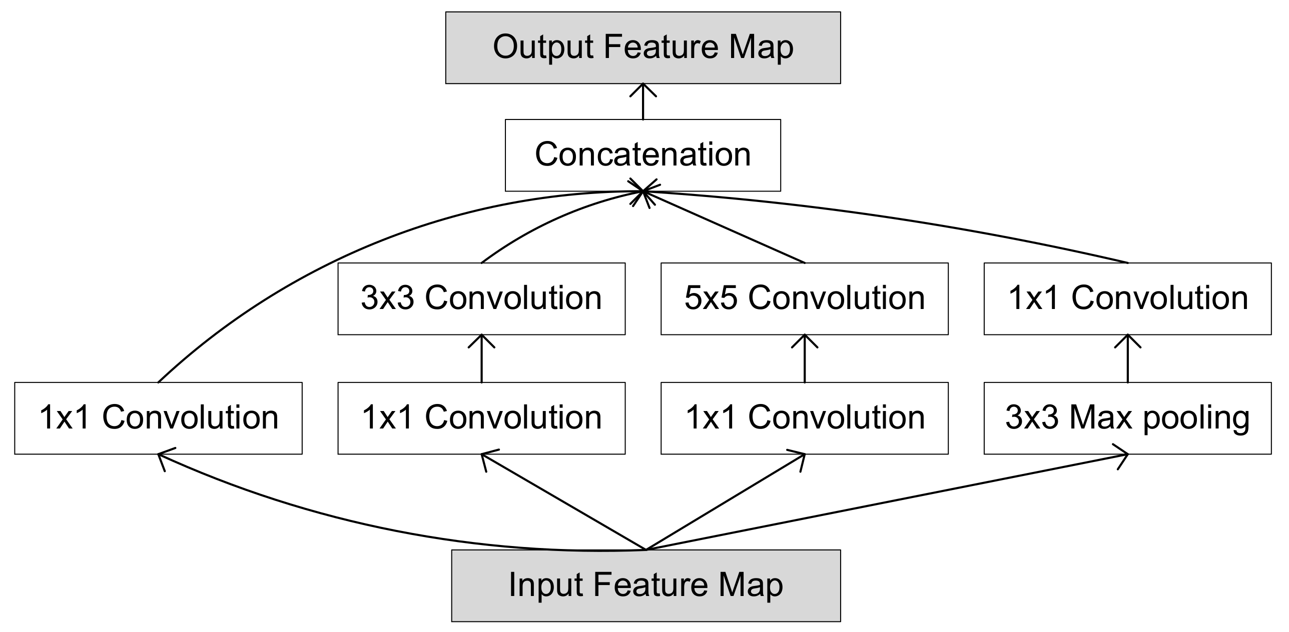
Table 1.
Comparison of cloud computing versus edge computing.
| Metric | Cloud Computing | Edge Computing |
|---|---|---|
| Computing Power | Cloud servers are powerful computing machines, | Edge servers and devices are computationally less powerful, |
| but shared by many users | but shared only in a limited area | |
| Latency | Services run faster in cloud servers, but the access to the servers is done | The proximity of edge servers and devices to the source of data improves the |
| through public communication networks with a high and variable latency | latency between service request and answer; it allows real-time services | |
| Bandwidth | Since all processing is done at the cloud, all data need to be transmitted to the | Since some or all of the processing is done at the edge, |
| cloud servers; therefore, it requires high communication bandwidth | close to the data source, it requires less communication bandwidth | |
| Cost | Cloud usage has a cost and requires a large costly bandwidth to | Local processing with edge servers |
| transfer data. Both increase with the addition of new data sources | and devices reduces communication costs | |
| Security | Transferring sensitive data to the cloud using public | Edge computing reduces data-sensitive transfer, |
| shared communication links reduces security and privacy | which increases security and keeps data private | |
| Services | Cloud services are offered at the application level to | Distributed and local computing allows services at |
| be generic enough to satisfy more customers | task level directed to specific needs of a user or customer | |
| Management | Central services are easier to manage; from the point of view of | Edge services are harder to manage since |
| the user, it offers a free management service | they are distributed and closer to the user | |
| Energy | Computing platforms of cloud centers are not | Edge and end devices are energy-constrained; |
| energy-constrained; the main goal is performance | performance is traded off with energy |
Table 2.
Summary of popular accuracy-oriented DNN models.
| Depth | Parameters (M) | Operations (G) | Top 5 Error (%) | Top- 1 Error (%) | |
|---|---|---|---|---|---|
| AlexNet | 8 | 61 | 1.45 | 15.4 | 36.7 |
| ZfNet | 8 | 60 | 1.47 | — | 36.0 |
| VGG16 | 16 | 138 | 31.0 | 8.1 | 25.6 |
| Inception-v1 | 22 | 5 | 2.86 | 10.1 | 30.2 |
| Inception-v2 | 42 | 11 | 4.0 | 7.8 | 25.2 |
| Inception-v3 | 48 | 24 | 11.4 | 5.6 | 21.2 |
| Inception-v4 | 76 | 35 | 24.5 | 4.9 | 19.9 |
| ResNet-152 | 152 | 60 | 22.6 | 4.5 | 19.4 |
| ResNeXt | 50 | 68 | 8.4 | 4.4 | 19.1 |
| DenseNet-201 | 201 | 20 | 8.4 | 6.4 | 23.6 |
Table 3.
Summary of lightweight DNN models.
| Model | Parameters (M) | Operations (G) | Top 5 Error (%) | Top 1 Error (%) |
|---|---|---|---|---|
| SqueezeNet | 1.2 | 1.72 | 19.7 | — |
| SqueezeNext | 3.2 | 1.42 | 11.8 | 32.5 |
| ShuffleNet x2 | 5.4 | 1.05 | 10.2 | 29.1 |
| MobileNetV1 | 4.2 | 1.15 | 10.5 | 29.4 |
| MobileNetV2 | 3.4 | 0.60 | 9.0 | 28.0 |
| MobileNetV3-Large | 5.4 | 0.44 | 7.8 | 24.8 |
| MobileNetV3-Small | 2.9 | 0.11 | 12.3 | 32.5 |
| CondenseNet G=C=4 | 2.9 | 0.55 | 10.0 | 29.0 |
| CondenseNet G=C=8 | 4.8 | 1.06 | 8.3 | 26.2 |
| NASNet-A | 5.3 | 1.13 | 8.4 | 26.0 |
| NASNet-B | 5.3 | 0.98 | 8.7 | 27.2 |
| NASNet-C | 4.9 | 1.12 | 9.0 | 27.5 |
| PNASNet | 5.1 | 1.18 | 8.1 | 25.7 |
| MNASNet-A1 | 3.9 | 0.62 | 7.5 | 24.8 |
| MNASNet-small | 2.0 | 0.14 | — | 34.0 |
| AmoebaNet-A | 5.1 | 1.11 | 8.0 | 25.5 |
| AmoebaNet-C | 6.4 | 1.14 | 7.6 | 24.3 |
| ANTNets | 3.7 | 0.64 | 8.8 | 26.8 |
| DARTS | 4.9 | 1.19 | 9.0 | 26.9 |
Table 4.
Summary of the most used data quantization and data reduction techniques.
| Data Quantization | |
|---|---|
| 16 bit floating-point | [113] |
| 8 bit floating-point | [114] |
| 8 bit fixed-point | [115,116,117,118] |
| <8 bit fixed-point | [119,120] |
| Hybrid fixed-point | [121,122,123] |
| Binary | [124,125,126,127] |
| Ternary | [128,129,130] |
| Data and Operation Reduction | |
| Pruning | [131,132,133,134,135,136] |
| Zero skipping | [137,139,140,141] |
| Batch | [142,143,144] |
| Winograd | [146,147,148,149,150] |
Table 5.
Summary of hardware accelerators for deep learning on the edge.
| Accelerator | Year | Model | GOPs | GOPs/W |
|---|---|---|---|---|
| ASIC Technology | ||||
| Gyrfalcon [151] | 2018 | CNN | 16.8 TOPs | 24 TOP/W |
| LinleyGroup [152] | 2018 | CNN | 12.5 TOPs | — |
| EV6x [153] | 2017 | DNN | 9.0 TOPs | 4 TOPs/W |
| Tensilica DNA [154] | 2017 | DNN | 24 TOPs | 6.8 TOPs/W |
| Myriad X [155] | 2017 | DNN | 4 TOPs | — |
| [156] | 2017 | CNN | — | 3.9 TOPs/W |
| Snapdragon 6 [157] | 2019 | DNN | 15 TOPs | 3 TOPs/W |
| Kirin 900 [158] | 2019 | DNN | 8 TOPs | — |
| Ascend 910 [159] | 2019 | DBB | 512 TOPs | 1.7 TOPs/W |
| Reconfigurable Computing Technology | ||||
| Eyeriss [161] | 2018 | CNN | 46.2 GOPs | 166 GOPs/W |
| Thinker chip [162] | 2018 | CNN | 368 GOPs | 1 TOPs/W |
| DRP [163] | 2018 | CNN | 960 GOPs | — |
| [167] | 2018 | CNN | 13 GOPs | — |
| [168] | 2018 | CNN | 84 GOPs | — |
| [169] | 2018 | CNN | 363 GOPs | 33 GOPs/W |
© 2020 by the authors. Licensee MDPI, Basel, Switzerland. This article is an open access article distributed under the terms and conditions of the Creative Commons Attribution (CC BY) license (http://creativecommons.org/licenses/by/4.0/).
Share and Cite
MDPI and ACS Style
Véstias, M.P.; Duarte, R.P.; de Sousa, J.T.; Neto, H.C. Moving Deep Learning to the Edge. Algorithms 2020, 13, 125. https://0-doi-org.brum.beds.ac.uk/10.3390/a13050125
AMA Style
Véstias MP, Duarte RP, de Sousa JT, Neto HC. Moving Deep Learning to the Edge. Algorithms. 2020; 13(5):125. https://0-doi-org.brum.beds.ac.uk/10.3390/a13050125
Chicago/Turabian StyleVéstias, Mário P., Rui Policarpo Duarte, José T. de Sousa, and Horácio C. Neto. 2020. "Moving Deep Learning to the Edge" Algorithms 13, no. 5: 125. https://0-doi-org.brum.beds.ac.uk/10.3390/a13050125
Note that from the first issue of 2016, this journal uses article numbers instead of page numbers. See further details here.