A Recursive Least-Squares Algorithm for the Identification of Trilinear Forms

Abstract

High-dimensional system identification problems can be efficiently addressed based on tensor decompositions and modelling. In this paper, we design a recursive least-squares (RLS) algorithm tailored for the identification of trilinear forms, namely RLS-TF. In our framework, the trilinear form is related to the decomposition of a third-order tensor (of rank one). The proposed RLS-TF algorithm acts on the individual components of the global impulse response, thus being efficient in terms of both performance and complexity. Simulation results indicate that the proposed solution outperforms the conventional RLS algorithm (which handles only the global impulse response), but also the previously developed trilinear counterparts based on the least-mean- squares algorithm.

1. Introduction

Currently, there is an increasing interest in developing methods and algorithms that exploit tensor decompositions and modelling [1,2]. These techniques become of significant importance in many real-world scenarios, e.g., when dealing with large amounts of data, processing multidimensional signals, or solving high-dimensional system identification problems. Many important applications rely on such tensor-based techniques, which can be successfully used in the fields of big data [3], source separation [4], machine learning [5], multiple-input multiple-output (MIMO) communication systems [6], and beamforming [7].

Tensor decompositions and their related applications are frequently addressed based on multilinear signal processing techniques [8,9]. For example, in the context of system identification scenarios, the problems can be formulated in terms of identifying multilinear forms. As particular cases, we can mention the bilinear and trilinear forms, where the decomposition is performed using two and three components, respectively. Since the Wiener filter and adaptive algorithms represent popular methods to address system identification problems, their applicability was also extended to the multilinear framework. Among the recent related works, we can mention the iterative Wiener filter for bilinear forms [10] and the subsequent adaptive filtering methods [11,12,13], together with their extensions to trilinear forms [14,15,16,17].

In this context, the work in [17] provided a system identification framework based on tensor decomposition, which was suitable for the trilinear approach. This work presents the iterative Wiener filter and least-mean-squares (LMS) adaptive algorithms tailored for trilinear forms. Among those, the normalized LMS (NLMS) algorithm for trilinear forms, namely NLMS-TF, represents a practical solution in terms of both performance and complexity. Nevertheless, it is known that the recursive least-squares (RLS) algorithm [18] could provide improved performance as compared to the LMS-based algorithms, especially in terms of the convergence rate. This represents the motivation behind the solution proposed in this paper, which targets the development of the RLS algorithm for trilinear forms, namely RLS-TF. Therefore, the goal of this work is mainly twofold. First, we aim to design a faster converging algorithm as compared to the recently developed NLMS-TF. Second, we intend to outline the performance features of the RLS-TF algorithm as compared to the conventional RLS benchmark.

Besides the conventional adaptive algorithms (which usually act as supervised methods), we should also note that unsupervised algorithms can be used in conjunction with tensor-based approaches, e.g., [19,20]. In this context, we can mention the single-channel blind source separation problem, which targets the identification of individual source signals from a single mixture recording. Such an approach can be found in [19], where the parameters of a so-called “imitated-stereo” mixture model (i.e., one real and the other virtual microphones, which results in an artificial mixing system of dual channels) were found by applying tensor estimation and exploiting sparsity features. The method proposed in [20] also exploits sparsity (using the Gibbs distribution) for multichannel source separation, by solving the underdetermined convolutive mixture separation, while considering the reverberations of the surrounding environment. Another appealing field where such tensor-based techniques can be applied is video processing. For example, unsupervised algorithms can be used for detecting anomalies in a video sequence, e.g., detecting micro defects while employing a thermography imaging system [21].

Currently, in many real-world applications related to MIMO systems, speech processing, and image/video processing, the received signals are tensors or can be grouped in a tensorial form. Consequently, as outlined before, utilizing estimation techniques from tensor algebra is beneficial. Moreover, in most of these applications, the underlying parameters to be estimated are sparse, so that specific features could be exploited, thus bringing additional advantages, especially for systems of large dimensions. The tensor-based RLS algorithm proposed in this paper represents an improved solution (in terms of convergence rate) as compared to the existing solution based on the NLMS algorithm [17], but also an efficient version (in terms of computational complexity) as compared to the conventional RLS algorithm [18].

The rest of the paper is organized as follows. Section 2 provides a background on third-order tensors, which represents the framework of trilinear forms. The proposed RLS-TF algorithm is developed in Section 3. Simulation results are provided in Section 4, outlining the main performance features of the designed solution. Finally, Section 5 concludes this paper and discusses several perspectives for future works.

2. Third-Order Tensors

In this section, we provide a brief summary on tensors, outlining the main definitions and operations, while also establishing the notation. A tensor can be defined as a multidimensional array of data [22,23]. For example, a matrix and a vector can be referred to as second- and first-order tensors, respectively. Tensors of order three or higher are called higher order tensors. In the following, the notation used for a tensor, a matrix, a vector, and a scalar is $\mathcal{A}$, $\mathbf{A}$, $\mathbf{a}$, and a, respectively. In this work, we are focusing only on real-valued third-order tensors, i.e., $\mathcal{A}\in {\mathbb{R}}^{L_1\times L_2\times L_3}$, so that the array dimension is $L_1\times L_2\times L_3$.

The entries of a tensor can be referred to by using multiple indices. In our case, for a third-order tensor, the first and second indices $l_1$ (with $l_1=1,2,\dots ,L_1$) and $l_2$ (with $l_2=1,2,\dots ,L_2$) correspond to the row and column, respectively (like in a matrix); in addition, the third index $l_3$ (with $l_3=1,2,\dots ,L_3$) corresponds to the tube and describes its depth. Consequently, these three indices describe the three different modes. In terms of notation, the entries of the different order tensors are denoted by ${\left(\mathcal{A}\right)}_{l_1{l}_2{l}_3}=a_{l_1{l}_2{l}_3}$, ${\left(\mathbf{A}\right)}_{l_1{l}_2}=a_{l_1{l}_2}$, and ${\left(\mathbf{a}\right)}_{l_1}=a_{l_1}$.

In the case of a matrix, the vectorization operation leads to a vector that contains the concatenated columns of the original matrix. In the case of a third-order tensor, the so-called matricization operation concatenates the “slices” of the tensor and produces a large matrix. Of course, the result depends on which index, all the elements of which are considered first. Thus, the matricization can be performed along three different modes [8,9]. For example, considering the mode row and then varying the columns and the tubes, we obtain:

$$\begin{array}{cc}\hfill {\mathbf{A}}_{\left[1\right]}& ={\mathbf{A}}_{:,1:L_2,1:L_3}\hfill \\ \hfill & =\left[\begin{array}{ccc}{\mathbf{A}}_{::1}& \cdots & {\mathbf{A}}_{::L_3}\end{array}\right],\hfill \end{array}$$

where ${\mathbf{A}}_{\left[1\right]}\in {\mathbb{R}}^{L_1\times L_2{L}_3}$ and the matrices ${\mathbf{A}}_{::l_3}\in {\mathbb{R}}^{L_1\times L_2}$ with $l_3=1,2\dots ,L_3$ denote the frontal slices. Similarly, we can take the mode column and then vary the lines and the tubes, which results in ${\mathbf{A}}_{\left[2\right]}={\mathbf{A}}_{1:L_1,:,1:L_3}$, with ${\mathbf{A}}_{\left[2\right]}\in {\mathbb{R}}^{L_2\times L_1{L}_3}$. Finally, we can take the mode tube and then vary the rows and the columns, in order to obtain ${\mathbf{A}}_{\left[3\right]}={\mathbf{A}}_{1:L_1,1:L_2,:}$, where ${\mathbf{A}}_{\left[3\right]}\in {\mathbb{R}}^{L_3\times L_1{L}_2}$. The ranks of ${\mathbf{A}}_{\left[1\right]}$, ${\mathbf{A}}_{\left[2\right]}$, and ${\mathbf{A}}_{\left[3\right]}$ represent the mode-1, mode-2, and mode-3 ranks of the tensor, respectively. Furthermore, the vectorization of a tensor (e.g., following mode-1) is

$$\begin{array}{cc}\hfill \mathrm{vec}\left(\mathcal{A}\right)& =\mathrm{vec}\left({\mathbf{A}}_{\left[1\right]}\right)\hfill \\ \hfill & =\left[\begin{array}{c}\mathrm{vec}\left({\mathbf{A}}_{::1}\right)\\ ⋮\\ \mathrm{vec}\left({\mathbf{A}}_{::L_3}\right)\end{array}\right]\in {\mathbb{R}}^{L_1{L}_2{L}_3}.\hfill \end{array}$$

Nevertheless, there are some fundamental differences between the rank of a matrix $\mathbf{A}\in {\mathbb{R}}^{L_1\times L_2}$ and the rank of a tensor $\mathcal{A}\in {\mathbb{R}}^{L_1\times L_2\times L_3}$. For example, the rank of $\mathbf{A}$ can never be larger than $\min \{L_1,L_2\}$, while the rank of $\mathcal{A}$ can be greater than $\min \{L_1,L_2,L_3\}$. A rank-1 tensor (of dimension $L_1\times L_2\times L_3$) is defined as:

$$\begin{array}{cc}\hfill \mathcal{B}& ={\mathbf{b}}_1\circ {\mathbf{b}}_2\circ {\mathbf{b}}_3,\hfill \end{array}$$

(1)

where ${\mathbf{b}}_1$, ${\mathbf{b}}_2$, and ${\mathbf{b}}_3$ are vectors of lengths $L_1$, $L_2$, and $L_3$, respectively, ∘ is the vector outer product, and the elements of $\mathcal{B}$ are given by ${\left(\mathcal{B}\right)}_{l_1{l}_2{l}_3}=b_{1,l_1}{b}_{2,l_2}{b}_{3,l_3}$, where $b_{i,l_i}$ are the elements of the vector ${\mathbf{b}}_i$, with $i=1,2,3$ and $l_i=1,2,\dots ,L_i$. In this case, it can be easily verified that:

$$\begin{array}{cc}\hfill \mathrm{vec}\left(\mathcal{B}\right)& ={\mathbf{b}}_3\otimes {\mathbf{b}}_2\otimes {\mathbf{b}}_1,\hfill \end{array}$$

(2)

where ⊗ denotes the Kronecker product [24]. In this context, the rank of a tensor $\mathcal{A}$, denoted $\mathrm{rank}\left(\mathcal{A}\right)$, is defined as the minimum number of rank-1 tensors that generate $\mathcal{A}$ as their sum. For example, if:

$$\begin{array}{cc}\hfill \mathcal{A}& =\sum _{r=1}^R{\mathbf{a}}_{1r}\circ {\mathbf{a}}_{2r}\circ {\mathbf{a}}_{3r},\hfill \end{array}$$

(3)

where ${\mathbf{a}}_{1r}$, ${\mathbf{a}}_{2r}$, and ${\mathbf{a}}_{3r}$ are vectors of lengths $L_1$, $L_2$, and $L_3$, respectively, then $\mathrm{rank}\left(\mathcal{A}\right)=R$ when R is minimal and (3) is called the canonical polyadic decomposition (CPD) of $\mathcal{A}$.

Another important operation is the multiplication of a tensor with a matrix [1,2], which can also be defined in different ways. For example, the mode-1 product between the tensor $\mathcal{A}\in {\mathbb{R}}^{L_1\times L_2\times L_3}$ and the matrix ${\mathbf{M}}_1\in {\mathbb{R}}^{M_1\times L_1}$ gives the tensor:

$$\begin{array}{cc}\hfill \mathcal{U}& =\mathcal{A}{\times }_1{\mathbf{M}}_1,\mathcal{U}\in {\mathbb{R}}^{M_1\times L_2\times L_3},\hfill \end{array}$$

(4)

whose entries are $u_{m_1{l}_2{l}_3}={\sum }_{l_1=1}^{L_1}{a}_{l_1{l}_2{l}_3}{m}_{m_1{l}_1}$ (for $m_1=1,2,\dots ,M_1$) and ${\mathbf{U}}_{\left[1\right]}={\mathbf{M}}_1{\mathbf{A}}_{\left[1\right]}$. Similarly, the mode-2 product between the same tensor $\mathcal{A}$ and the matrix ${\mathbf{M}}_2\in {\mathbb{R}}^{M_2\times L_2}$ leads to the tensor:

$$\begin{array}{cc}\hfill \underline{\mathcal{U}}& =\mathcal{A}{\times }_2{\mathbf{M}}_2,\underline{\mathcal{U}}\in {\mathbb{R}}^{L_1\times M_2\times L_3},\hfill \end{array}$$

(5)

with the entries ${\underline{u}}_{l_1{m}_2{l}_3}={\sum }_{l_2=1}^{L_2}{a}_{l_1{l}_2{l}_3}{m}_{m_2{l}_2}$ (for $m_2=1,2,\dots ,M_2$) and ${\underline{\mathbf{U}}}_{\left[2\right]}={\mathbf{M}}_2{\mathbf{A}}_{\left[2\right]}$. Finally, the mode-3 product between the tensor $\mathcal{A}$ and the matrix ${\mathbf{M}}_3\in {\mathbb{R}}^{M_3\times L_3}$ results in the tensor:

$$\begin{array}{cc}\hfill \overline{\mathcal{U}}& =\mathcal{A}{\times }_3{\mathbf{M}}_3,\overline{\mathcal{U}}\in {\mathbb{R}}^{L_1\times L_2\times M_3},\hfill \end{array}$$

(6)

having the entries ${\overline{u}}_{l_1{l}_2{m}_3}={\sum }_{l_3=1}^{L_3}{a}_{l_1{l}_2{l}_3}{m}_{m_3{l}_3}$ (for $m_3=1,2,\dots ,M_3$), while ${\overline{\mathbf{U}}}_{\left[3\right]}={\mathbf{M}}_3{\mathbf{A}}_{\left[3\right]}$. Clearly, we can multiply the tensor $\mathcal{A}$ with the three previously defined matrices ${\mathbf{M}}_1$, ${\mathbf{M}}_2$, and ${\mathbf{M}}_3$. In this case, we get the tensor:

$$\begin{array}{cc}\hfill \mathcal{T}& =\mathcal{A}{\times }_1{\mathbf{M}}_1{\times }_2{\mathbf{M}}_2{\times }_3{\mathbf{M}}_3\hfill \\ \hfill & =\mathcal{A}{\times }_1{\mathbf{M}}_1{\times }_3{\mathbf{M}}_3{\times }_2{\mathbf{M}}_2\hfill \\ \hfill & =\mathcal{A}{\times }_2{\mathbf{M}}_2{\times }_1{\mathbf{M}}_1{\times }_3{\mathbf{M}}_3\hfill \\ \hfill & =\mathcal{A}{\times }_2{\mathbf{M}}_2{\times }_3{\mathbf{M}}_3{\times }_1{\mathbf{M}}_1\hfill \\ \hfill & =\mathcal{A}{\times }_3{\mathbf{M}}_3{\times }_1{\mathbf{M}}_1{\times }_2{\mathbf{M}}_2\hfill \\ \hfill & =\mathcal{A}{\times }_3{\mathbf{M}}_3{\times }_2{\mathbf{M}}_2{\times }_1{\mathbf{M}}_1,\hfill \end{array}$$

(7)

where $\mathcal{T}\in {\mathbb{R}}^{M_1\times M_2\times M_3}$. As a consequence, considering ${\mathbf{b}}_1$, ${\mathbf{b}}_2$, and ${\mathbf{b}}_3$ three vectors of lengths $L_1$, $L_2$, and $L_3$, respectively, the multiplication of the tensor $\mathcal{A}$ with the transposed vectors gives the scalar:

$$\begin{array}{cc}\hfill c& =\mathcal{A}{\times }_1{\mathbf{b}}_1^T{\times }_2{\mathbf{b}}_2^T{\times }_3{\mathbf{b}}_3^T\hfill \\ \hfill & =\sum _{l_1=1}^{L_1}\sum _{l_2=1}^{L_2}\sum _{l_3=1}^{L_3}{a}_{l_1{l}_2{l}_3}{b}_{1l_1}{b}_{2l_2}{b}_{3l_3},\hfill \end{array}$$

(8)

where ${}^T$ is the transpose operator. It is easy to check that (8) is trilinear with respect to ${\mathbf{b}}_1$, ${\mathbf{b}}_2$, and ${\mathbf{b}}_3$.

At this point, we can also define the inner product between two tensors $\mathcal{A}$ and $\mathcal{B}$ of the same dimension ($L_1\times L_2\times L_3$), which is:

$$\begin{array}{cc}\hfill \langle \mathcal{A},\mathcal{B}\rangle & =\sum _{l_1=1}^{L_1}\sum _{l_2=1}^{L_2}\sum _{l_3=1}^{L_3}{a}_{l_1{l}_2{l}_3}{b}_{l_1{l}_2{l}_3}\hfill \\ \hfill & ={\mathrm{vec}}^T\left(\mathcal{B}\right)\mathrm{vec}\left(\mathcal{A}\right).\hfill \end{array}$$

(9)

Therefore, Expression (8) can also be written in a more convenient way, i.e.,

$$\begin{array}{cc}\hfill c& =\langle \mathcal{A},\mathcal{B}\rangle \hfill \\ \hfill & ={\mathrm{vec}}^T\left(\mathcal{B}\right)\mathrm{vec}\left(\mathcal{A}\right)\hfill \\ \hfill & ={\mathrm{vec}}^T\left({\mathbf{b}}_1\circ {\mathbf{b}}_2\circ {\mathbf{b}}_3\right)\mathrm{vec}\left(\mathcal{A}\right)\hfill \\ \hfill & ={\left({\mathbf{b}}_3\otimes {\mathbf{b}}_2\otimes {\mathbf{b}}_1\right)}^T\mathrm{vec}\left(\mathcal{A}\right),\hfill \end{array}$$

(10)

where $\mathcal{B}={\mathbf{b}}_1\circ {\mathbf{b}}_2\circ {\mathbf{b}}_3$ (see (1)). Moreover, if $\mathcal{A}$ is also a rank-1 tensor, i.e., $\mathcal{A}={\mathbf{a}}_1\circ {\mathbf{a}}_2\circ {\mathbf{a}}_3$, where the vectors ${\mathbf{a}}_i$ have the lengths $L_i$ (with $i=1,2,3$), then:

$$\begin{array}{cc}\hfill \langle \mathcal{A},\mathcal{B}\rangle & ={\mathbf{b}}_1^T{\mathbf{a}}_1\times {\mathbf{b}}_2^T{\mathbf{a}}_2\times {\mathbf{b}}_3^T{\mathbf{a}}_3.\hfill \end{array}$$

(11)

Furthermore, it is easy to check that:

$$\begin{array}{cc}\hfill \mathcal{B}{\times }_1{\mathbf{M}}_1& ={\mathbf{M}}_1{\mathbf{b}}_1\circ {\mathbf{b}}_2\circ {\mathbf{b}}_3,\hfill \\ \hfill \mathcal{B}{\times }_2{\mathbf{M}}_2& ={\mathbf{b}}_1\circ {\mathbf{M}}_2{\mathbf{b}}_2\circ {\mathbf{b}}_3,\hfill \\ \hfill \mathcal{B}{\times }_3{\mathbf{M}}_3& ={\mathbf{b}}_1\circ {\mathbf{b}}_2\circ {\mathbf{M}}_3{\mathbf{b}}_3,\hfill \end{array}$$

where the matrices ${\mathbf{M}}_1$, ${\mathbf{M}}_2$, and ${\mathbf{M}}_3$ were previously defined (related to (4)–(6)).

The short background on tensors provided before and the main related operations (e.g., matricization, vectorization, rank, and different types of product) aim to facilitate the development that follows in Section 3. It is also important to outline that the trilinear forms result in the context of the decomposition of third-order tensors. Extension to higher order tensors and multilinear forms could be straightforward when dealing with rank-1 tensors. Otherwise, in the general case, decomposing higher rank higher order tensors (see (3)) raises additional difficulties, as will be briefly pointed out at the end of Section 5.

3. RLS Algorithm for Trilinear Forms

In the following, for the sake of consistency with the development of the NLMS-TF algorithm, we will keep the framework and notation from [17]. Therefore, let us consider the output of a multiple-input single-output (MISO) system (with real-valued data) at the discrete-time index n defined as:

$$\begin{array}{cc}\hfill y\left(n\right)& =\mathcal{X}\left(n\right){\times }_1{\mathbf{h}}_1^T{\times }_2{\mathbf{h}}_2^T{\times }_3{\mathbf{h}}_3^T\hfill \\ \hfill & =\sum _{l_1=1}^{L_1}\sum _{l_2=1}^{L_2}\sum _{l_3=1}^{L_3}{x}_{l_1{l}_2{l}_3}\left(n\right)h_{1,l_1}{h}_{2,l_2}{h}_{3,l_3},\hfill \end{array}$$

(12)

where the tensorial form $\mathcal{X}\left(n\right)\in {\mathbb{R}}^{L_1\times L_2\times L_3}$ groups the input signals, with:

$$\begin{array}{cc}\hfill {\left[\mathcal{X}\left(n\right)\right]}_{l_1{l}_2{l}_3}& =x_{l_1{l}_2{l}_3}\left(n\right),l_i=1,2,\dots ,L_i,i=1,2,3,\hfill \end{array}$$

and the vectors ${\mathbf{h}}_i,i=1,2,3$ (of lengths $L_1$, $L_2$, and $L_3$, respectively) define the three impulse responses, i.e.,

$$\begin{array}{c}\hfill {\mathbf{h}}_i={\left[\begin{array}{cccc}{h}_{i,1}& h_{i,2}& \cdots & h_{i,L_i}\end{array}\right]}^T,i=1,2,3.\end{array}$$

As we can notice, $y\left(n\right)$ represents a trilinear form (see (12) as compared to (8)), because it is a linear function of each of the vectors ${\mathbf{h}}_i,i=1,2,3$, if the other two are fixed.

Next, we can also introduce a rank-1 tensor of dimension $L_1\times L_2\times L_3$, using the three impulse responses of the MISO system:

$$\begin{array}{cc}\hfill \mathcal{H}& ={\mathbf{h}}_1\circ {\mathbf{h}}_2\circ {\mathbf{h}}_3,\hfill \end{array}$$

(13)

whose elements are:

$$\begin{array}{cc}\hfill {\left(\mathcal{H}\right)}_{l_1{l}_2{l}_3}& =h_{1,l_1}{h}_{2,l_2}{h}_{3,l_3},l_i=1,2,\dots ,L_i,i=1,2,3.\hfill \end{array}$$

Consequently, the output signal results in:

$$\begin{array}{c}\hfill y\left(n\right)={\mathrm{vec}}^T\left(\mathcal{H}\right)\mathrm{vec}\left[\mathcal{X}\left(n\right)\right],\end{array}$$

(14)

where:

$$\begin{array}{cc}\hfill \mathrm{vec}\left(\mathcal{H}\right)& =\left[\begin{array}{c}\mathrm{vec}\left({\mathbf{H}}_{::1}\right)\\ ⋮\\ \mathrm{vec}\left({\mathbf{H}}_{::L_3}\right)\end{array}\right],\hfill \end{array}$$

(15)

$$\begin{array}{cc}\hfill \mathrm{vec}\left[\mathcal{X}\left(n\right)\right]& =\left[\begin{array}{c}\mathrm{vec}\left[{\mathbf{X}}_{::1}\left(n\right)\right]\\ ⋮\\ \mathrm{vec}\left[{\mathbf{X}}_{::L_3}\left(n\right)\right]\end{array}\right],\hfill \end{array}$$

(16)

with ${\mathbf{H}}_{::l_3}$ and ${\mathbf{X}}_{::l_3}\left(n\right)$ ($l_3=1,2\dots ,L_3$) being the frontal slices of $\mathcal{H}$ and $\mathcal{X}\left(n\right)$, respectively. At this point, we can introduce the notation:

$$\begin{array}{cc}\hfill \mathbf{h}& \triangleq \mathrm{vec}\left(\mathcal{H}\right)={\mathbf{h}}_3\otimes {\mathbf{h}}_2\otimes {\mathbf{h}}_1,\hfill \end{array}$$

(17)

$$\begin{array}{cc}\hfill \mathbf{x}\left(n\right)& \triangleq \mathrm{vec}\left[\mathcal{X}\left(n\right)\right],\hfill \end{array}$$

(18)

where $\mathbf{h}$ and $\mathbf{x}\left(n\right)$ are two long vectors, each of them having $L_1{L}_2{L}_3$ elements. Thus, the output signal can also be expressed as:

$$\begin{array}{c}\hfill y\left(n\right)={\mathbf{h}}^T\mathbf{x}\left(n\right).\end{array}$$

(19)

The main goal is to estimate the output of the MISO system, which is usually corrupted by an additive noise. Hence, the reference signal results in:

$$\begin{array}{cc}\hfill d\left(n\right)& =y\left(n\right)+w\left(n\right)\hfill \\ \hfill & ={\mathbf{h}}^T\mathbf{x}\left(n\right)+w\left(n\right),\hfill \end{array}$$

(20)

where $w\left(n\right)$ is a zero-mean additive noise, which is uncorrelated with the input signals. Alternatively, we could estimate the global impulse response $\mathbf{h}$, using an adaptive filter $\widehat{\mathbf{h}}\left(n\right)$ (of length $L_1{L}_2{L}_3$). At this point, we may also define the error signal:

$$\begin{array}{cc}\hfill e\left(n\right)& =d\left(n\right)-\widehat{y}\left(n\right)\hfill \\ \hfill & =d\left(n\right)-{\widehat{\mathbf{h}}}^T(n-1)\mathbf{x}\left(n\right),\hfill \end{array}$$

(21)

which represents the difference between the reference signal and the estimated signal, $\widehat{y}\left(n\right)$.

Based on (17), we can notice that the global impulse response $\mathbf{h}$ (of length $L_1{L}_2{L}_3$) results based on a combination of the shorter impulse responses ${\mathbf{h}}_i,i=1,2,3$, of lengths $L_1$, $L_2$, and $L_3$, respectively. Consequently, the estimated impulse response can also be decomposed as:

$$\begin{array}{c}\hfill \widehat{\mathbf{h}}\left(n\right)={\widehat{\mathbf{h}}}_3\left(n\right)\otimes {\widehat{\mathbf{h}}}_2\left(n\right)\otimes {\widehat{\mathbf{h}}}_1\left(n\right),\end{array}$$

(22)

where ${\widehat{\mathbf{h}}}_i\left(n\right),i=1,2,3$ are three adaptive filters (with $L_1$, $L_2$, and $L_3$ coefficients, respectively), which aim to model the individual impulse responses ${\mathbf{h}}_i,i=1,2,3$. Nevertheless, we should notice that there is no unique solution related to the decomposition in (22). It is obvious that, for any constants ${\eta }_1,{\eta }_2$, and ${\eta }_3$, with ${\eta }_1{\eta }_2{\eta }_3=1$, we have:

$$\begin{array}{cc}\hfill \mathbf{h}& ={\mathbf{h}}_3\otimes {\mathbf{h}}_2\otimes {\mathbf{h}}_1\hfill \\ \hfill & ={\eta }_3{\mathbf{h}}_3\otimes {\eta }_2{\mathbf{h}}_2\otimes {\eta }_1{\mathbf{h}}_1.\hfill \end{array}$$

(23)

Hence, ${\eta }_i{\mathbf{h}}_i,i=1,2,3$ also represent a set of solutions. However, the global impulse response $\mathbf{h}$ is identified with no scaling ambiguity.

Following the decomposition from (22), we can easily verify that:

$$\begin{array}{cc}\hfill \widehat{\mathbf{h}}\left(n\right)& ={\widehat{\mathbf{H}}}_{32}\left(n\right){\widehat{\mathbf{h}}}_1\left(n\right)\hfill \end{array}$$

(24)

$$\begin{array}{cc}\hfill & ={\widehat{\mathbf{H}}}_{31}\left(n\right){\widehat{\mathbf{h}}}_2\left(n\right)\hfill \end{array}$$

(25)

$$\begin{array}{cc}\hfill & ={\widehat{\mathbf{H}}}_{21}\left(n\right){\widehat{\mathbf{h}}}_3\left(n\right),\hfill \end{array}$$

(26)

where:

$$\begin{array}{cc}\hfill {\widehat{\mathbf{H}}}_{32}\left(n\right)& ={\widehat{\mathbf{h}}}_3\left(n\right)\otimes {\widehat{\mathbf{h}}}_2\left(n\right)\otimes {\mathbf{I}}_{L_1},\hfill \end{array}$$

(27)

$$\begin{array}{cc}\hfill {\widehat{\mathbf{H}}}_{31}\left(n\right)& ={\widehat{\mathbf{h}}}_3\left(n\right)\otimes {\mathbf{I}}_{L_2}\otimes {\widehat{\mathbf{h}}}_1\left(n\right),\hfill \end{array}$$

(28)

$$\begin{array}{cc}\hfill {\widehat{\mathbf{H}}}_{21}\left(n\right)& ={\mathbf{I}}_{L_3}\otimes {\widehat{\mathbf{h}}}_2\left(n\right)\otimes {\widehat{\mathbf{h}}}_1\left(n\right),\hfill \end{array}$$

(29)

and ${\mathbf{I}}_{L_i},i=1,2,3$ are the identity matrices of sizes $L_1\times L_1$, $L_2\times L_2$, and $L_3\times L_3$, respectively. Moreover, introducing the notation:

$$\begin{array}{cc}\hfill {\mathbf{x}}_{32}\left(n\right)& ={\widehat{\mathbf{H}}}_{32}^T(n-1)\mathbf{x}\left(n\right),\hfill \end{array}$$

(30)

$$\begin{array}{cc}\hfill {\mathbf{x}}_{31}\left(n\right)& ={\widehat{\mathbf{H}}}_{31}^T(n-1)\mathbf{x}\left(n\right),\hfill \end{array}$$

(31)

$$\begin{array}{cc}\hfill {\mathbf{x}}_{21}\left(n\right)& ={\widehat{\mathbf{H}}}_{21}^T(n-1)\mathbf{x}\left(n\right),\hfill \end{array}$$

(32)

the error signal from (21) can be expressed in three equivalent ways as:

$$\begin{array}{cc}\hfill e\left(n\right)& =d\left(n\right)-{\widehat{\mathbf{h}}}_1^T(n-1){\mathbf{x}}_{32}\left(n\right),\hfill \end{array}$$

(33)

$$\begin{array}{cc}\hfill & =d\left(n\right)-{\widehat{\mathbf{h}}}_2^T(n-1){\mathbf{x}}_{31}\left(n\right),\hfill \end{array}$$

(34)

$$\begin{array}{cc}\hfill & =d\left(n\right)-{\widehat{\mathbf{h}}}_3^T(n-1){\mathbf{x}}_{21}\left(n\right).\hfill \end{array}$$

(35)

Based on the least-squares error criterion [18] applied in the context of (20) and (21), the conventional RLS algorithm is derived from:

$$\begin{array}{cc}\hfill J\left[\widehat{\mathbf{h}}\left(n\right)\right]& =\sum _{i=1}^n{\lambda }^{n-i}{\left[d\left(i\right)-{\widehat{\mathbf{h}}}^T\left(n\right)\mathbf{x}\left(i\right)\right]}^2,\hfill \end{array}$$

(36)

where $\lambda \le 1$ is a positive constant known as the forgetting factor. On the other hand, based on (24)–(26), the cost function from (36) can be expressed in three different ways, targeting the optimization of the individual components, i.e.,

$$\begin{array}{cc}\hfill J_{{\widehat{\mathbf{h}}}_3,{\widehat{\mathbf{h}}}_2}\left[{\widehat{\mathbf{h}}}_1\left(n\right)\right]& =\sum _{i=1}^n{\lambda }_1^{n-i}{\left[d\left(i\right)-{\widehat{\mathbf{h}}}_1^T\left(n\right){\mathbf{x}}_{32}\left(i\right)\right]}^2,\hfill \end{array}$$

(37)

$$\begin{array}{cc}\hfill J_{{\widehat{\mathbf{h}}}_3,{\widehat{\mathbf{h}}}_1}\left[{\widehat{\mathbf{h}}}_2\left(n\right)\right]& =\sum _{i=1}^n{\lambda }_2^{n-i}{\left[d\left(i\right)-{\widehat{\mathbf{h}}}_2^T\left(n\right){\mathbf{x}}_{31}\left(i\right)\right]}^2,\hfill \end{array}$$

(38)

$$\begin{array}{cc}\hfill J_{{\widehat{\mathbf{h}}}_2,{\widehat{\mathbf{h}}}_1}\left[{\widehat{\mathbf{h}}}_3\left(n\right)\right]& =\sum _{i=1}^n{\lambda }_3^{n-i}{\left[d\left(i\right)-{\widehat{\mathbf{h}}}_3^T\left(n\right){\mathbf{x}}_{21}\left(i\right)\right]}^2,\hfill \end{array}$$

(39)

where ${\lambda }_1$, ${\lambda }_2$, and ${\lambda }_3$ are the individual forgetting factors. The previous cost functions suggest a “trilinear” optimization strategy [25], where we assume that two components are fixed during the optimization of the third one. Consequently, based on the minimization of (37)–(39) with respect to ${\widehat{\mathbf{h}}}_1\left(n\right)$, ${\widehat{\mathbf{h}}}_2\left(n\right)$, and ${\widehat{\mathbf{h}}}_3\left(n\right)$, respectively, the following set of normal equations are obtained:

$$\begin{array}{cc}\hfill {\mathbf{R}}_{32}\left(n\right){\widehat{\mathbf{h}}}_1\left(n\right)& ={\mathbf{p}}_{32}\left(n\right),\hfill \end{array}$$

(40)

$$\begin{array}{cc}\hfill {\mathbf{R}}_{31}\left(n\right){\widehat{\mathbf{h}}}_2\left(n\right)& ={\mathbf{p}}_{31}\left(n\right),\hfill \end{array}$$

(41)

$$\begin{array}{cc}\hfill {\mathbf{R}}_{21}\left(n\right){\widehat{\mathbf{h}}}_3\left(n\right)& ={\mathbf{p}}_{21}\left(n\right),\hfill \end{array}$$

(42)

where:

$$\begin{array}{cc}\hfill {\mathbf{R}}_{32}\left(n\right)& =\sum _{i=1}^n{\lambda }_1^{n-i}{\mathbf{x}}_{32}\left(i\right){\mathbf{x}}_{32}^T\left(i\right)\hfill \\ \hfill & ={\lambda }_1{\mathbf{R}}_{32}(n-1)+{\mathbf{x}}_{32}\left(n\right){\mathbf{x}}_{32}^T\left(n\right),\hfill \\ \hfill {\mathbf{p}}_{32}\left(n\right)& =\sum _{i=1}^n{\lambda }_1^{n-i}{\mathbf{x}}_{32}\left(i\right)d\left(i\right)\hfill \\ \hfill & ={\lambda }_1{\mathbf{p}}_{32}(n-1)+{\mathbf{x}}_{32}\left(n\right)d\left(n\right),\hfill \\ \hfill {\mathbf{R}}_{31}\left(n\right)& =\sum _{i=1}^n{\lambda }_2^{n-i}{\mathbf{x}}_{31}\left(i\right){\mathbf{x}}_{31}^T\left(i\right)\hfill \\ \hfill & ={\lambda }_2{\mathbf{R}}_{31}(n-1)+{\mathbf{x}}_{31}\left(n\right){\mathbf{x}}_{31}^T\left(n\right),\hfill \\ \hfill {\mathbf{p}}_{31}\left(n\right)& =\sum _{i=1}^n{\lambda }_2^{n-i}{\mathbf{x}}_{31}\left(i\right)d\left(i\right)\hfill \\ \hfill & ={\lambda }_2{\mathbf{p}}_{31}(n-1)+{\mathbf{x}}_{31}\left(n\right)d\left(n\right),\hfill \\ \hfill {\mathbf{R}}_{21}\left(n\right)& =\sum _{i=1}^n{\lambda }_3^{n-i}{\mathbf{x}}_{21}\left(i\right){\mathbf{x}}_{21}^T\left(i\right)\hfill \\ \hfill & ={\lambda }_2{\mathbf{R}}_{21}(n-1)+{\mathbf{x}}_{21}\left(n\right){\mathbf{x}}_{21}^T\left(n\right),\hfill \\ \hfill {\mathbf{p}}_{21}\left(n\right)& =\sum _{i=1}^n{\lambda }_3^{n-i}{\mathbf{x}}_{21}\left(i\right)d\left(i\right)\hfill \\ \hfill & ={\lambda }_3{\mathbf{p}}_{21}(n-1)+{\mathbf{x}}_{21}\left(n\right)d\left(n\right).\hfill \end{array}$$

Solving (40)–(42), the updates of the individual filters result in:

$$\begin{array}{cc}\hfill {\widehat{\mathbf{h}}}_1\left(n\right)& ={\widehat{\mathbf{h}}}_1(n-1)+{\mathbf{R}}_{32}^{-1}\left(n\right){\mathbf{x}}_{32}\left(n\right)e\left(n\right)\hfill \\ \hfill & ={\widehat{\mathbf{h}}}_1(n-1)+{\mathbf{k}}_{32}\left(n\right)e\left(n\right),\hfill \end{array}$$

(43)

$$\begin{array}{cc}\hfill {\widehat{\mathbf{h}}}_2\left(n\right)& ={\widehat{\mathbf{h}}}_2(n-1)+{\mathbf{R}}_{31}^{-1}\left(n\right){\mathbf{x}}_{31}\left(n\right)e\left(n\right)\hfill \\ \hfill & ={\widehat{\mathbf{h}}}_2(n-1)+{\mathbf{k}}_{31}\left(n\right)e\left(n\right),\hfill \end{array}$$

(44)

$$\begin{array}{cc}\hfill {\widehat{\mathbf{h}}}_3\left(n\right)& ={\widehat{\mathbf{h}}}_3(n-1)+{\mathbf{R}}_{21}^{-1}\left(n\right){\mathbf{x}}_{21}\left(n\right)e\left(n\right)\hfill \\ \hfill & ={\widehat{\mathbf{h}}}_3(n-1)+{\mathbf{k}}_{21}\left(n\right)e\left(n\right),\hfill \end{array}$$

(45)

where ${\mathbf{k}}_{32}\left(n\right)={\mathbf{R}}_{32}^{-1}\left(n\right){\mathbf{x}}_{32}\left(n\right)$, ${\mathbf{k}}_{31}\left(n\right)={\mathbf{R}}_{31}^{-1}\left(n\right){\mathbf{x}}_{31}\left(n\right)$, and ${\mathbf{k}}_{21}\left(n\right)={\mathbf{R}}_{21}^{-1}\left(n\right){\mathbf{x}}_{21}\left(n\right)$ are the Kalman gain vectors, while the error signal can be computed based on (33). At this point, the main task is to update the inverse of the matrices ${\mathbf{R}}_{32}\left(n\right)$, ${\mathbf{R}}_{31}\left(n\right)$, and ${\mathbf{R}}_{21}\left(n\right)$ efficiently. The solution relies on the matrix inversion lemma [18], which leads to the following updates:

$$\begin{array}{cc}\hfill {\mathbf{R}}_{32}^{-1}\left(n\right)& =\frac{1}{{\lambda }_1}\left[{\mathbf{I}}_{L_1}-{\mathbf{k}}_{32}\left(n\right){\mathbf{x}}_{32}^T\left(n\right)\right]{\mathbf{R}}_{32}^{-1}(n-1),\hfill \end{array}$$

(46)

$$\begin{array}{cc}\hfill {\mathbf{R}}_{31}^{-1}\left(n\right)& =\frac{1}{{\lambda }_2}\left[{\mathbf{I}}_{L_2}-{\mathbf{k}}_{31}\left(n\right){\mathbf{x}}_{31}^T\left(n\right)\right]{\mathbf{R}}_{31}^{-1}(n-1),\hfill \end{array}$$

(47)

$$\begin{array}{cc}\hfill {\mathbf{R}}_{21}^{-1}\left(n\right)& =\frac{1}{{\lambda }_3}\left[{\mathbf{I}}_{L_3}-{\mathbf{k}}_{21}\left(n\right){\mathbf{x}}_{21}^T\left(n\right)\right]{\mathbf{R}}_{21}^{-1}(n-1).\hfill \end{array}$$

(48)

Therefore, the Kalman gain vectors are evaluated as:

$$\begin{array}{cc}\hfill {\mathbf{k}}_{32}\left(n\right)& =\frac{{\mathbf{R}}_{32}^{-1}(n-1){\mathbf{x}}_{32}\left(n\right)}{{\lambda }_1+{\mathbf{x}}_{32}^T\left(n\right){\mathbf{R}}_{32}^{-1}(n-1){\mathbf{x}}_{32}\left(n\right)},\hfill \end{array}$$

(49)

$$\begin{array}{cc}\hfill {\mathbf{k}}_{31}\left(n\right)& =\frac{{\mathbf{R}}_{31}^{-1}(n-1){\mathbf{x}}_{31}\left(n\right)}{{\lambda }_2+{\mathbf{x}}_{31}^T\left(n\right){\mathbf{R}}_{31}^{-1}(n-1){\mathbf{x}}_{31}\left(n\right)},\hfill \end{array}$$

(50)

$$\begin{array}{cc}\hfill {\mathbf{k}}_{21}\left(n\right)& =\frac{{\mathbf{R}}_{21}^{-1}(n-1){\mathbf{x}}_{21}\left(n\right)}{{\lambda }_3+{\mathbf{x}}_{21}^T\left(n\right){\mathbf{R}}_{21}^{-1}(n-1){\mathbf{x}}_{21}\left(n\right)}.\hfill \end{array}$$

(51)

For initialization, we can choose:

$$\begin{array}{cc}\hfill {\widehat{\mathbf{h}}}_1\left(0\right)& =\left[\begin{array}{c}1\hfill \\ {\mathbf{0}}_{L_1-1}\hfill \end{array}\right],\hfill \end{array}$$

(52)

$$\begin{array}{cc}\hfill {\widehat{\mathbf{h}}}_2\left(0\right)& =\frac{1}{L_2}{\mathbf{1}}_{L_2},\hfill \end{array}$$

(53)

$$\begin{array}{cc}\hfill {\widehat{\mathbf{h}}}_3\left(0\right)& =\frac{1}{L_3}{\mathbf{1}}_{L_3},\hfill \end{array}$$

(54)

where ${\mathbf{0}}_N$ and ${\mathbf{1}}_N$ are two vectors of length N, all elements of which are equal to zero and one, respectively.

The proposed RLS algorithm for trilinear forms, namely RLS-TF, is summarized in

Table 1. RLS algorithm for trilinear forms (RLS-TF).

Initialization:

Set ${\widehat{\mathbf{h}}}_1\left(0\right)$, ${\widehat{\mathbf{h}}}_2\left(0\right)$, and ${\widehat{\mathbf{h}}}_3\left(0\right)$ based on (52)–(54)

${\mathbf{R}}_{32}^{-1}\left(0\right)=\frac{1}{{\delta }_1}{\mathbf{I}}_{L_1},{\mathbf{R}}_{31}^{-1}\left(0\right)=\frac{1}{{\delta }_2}{\mathbf{I}}_{L_2},{\mathbf{R}}_{21}^{-1}\left(0\right)=\frac{1}{{\delta }_3}{\mathbf{I}}_{L_3}$

$\left(\mathrm{Regularization} \mathrm{parameters}:{\delta }_1>0,{\delta }_2>0,{\delta }_3>0\right)$

${\lambda }_1=1-\frac{1}{K{L}_1},{\lambda }_2=1-\frac{1}{K{L}_2},{\lambda }_3=1-\frac{1}{K{L}_3}$

$\left(\mathrm{Tuning}\mathrm{constant}:K\ge 1\right)$

$\mathrm{For}n=1,2,\dots ,\mathrm{number}\mathrm{of}\mathrm{iterations}:$

Compute ${\widehat{\mathbf{H}}}_{32}(n-1)$, ${\widehat{\mathbf{H}}}_{31}(n-1)$, and ${\widehat{\mathbf{H}}}_{21}(n-1)$ based on (27)–(29)

Compute ${\mathbf{x}}_{32}\left(n\right)$, ${\mathbf{x}}_{31}\left(n\right)$, and ${\mathbf{x}}_{21}\left(n\right)$ based on (30)–(32)

Evaluate the error signal $e\left(n\right)$ based on (33)

Compute ${\mathbf{k}}_{32}\left(n\right)$, ${\mathbf{k}}_{31}\left(n\right)$, and ${\mathbf{k}}_{21}\left(n\right)$ based on (49)–(51)

Update ${\widehat{\mathbf{h}}}_1\left(n\right)$, ${\widehat{\mathbf{h}}}_2\left(n\right)$, and ${\widehat{\mathbf{h}}}_3\left(n\right)$ based on (43)–(45)

Update ${\mathbf{R}}_{32}^{-1}\left(n\right)$, ${\mathbf{R}}_{31}^{-1}\left(n\right)$, and ${\mathbf{R}}_{21}^{-1}\left(n\right)$ based on (46)–(48)

Evaluate $\widehat{\mathbf{h}}\left(n\right)$ based on (22)

. It could also be interpreted as an extension of the RLS-based algorithm tailored for bilinear forms, which was presented in [12]. However, if the MISO system identification problem results based on (12), it is natural to use the RLS-TF algorithm, which is designed for the identification of third-order (rank-1) tensors.

In terms of computational complexity, it can be noticed that the proposed RLS-TF algorithm combines the solutions provided by three RLS-based filters, i.e., ${\widehat{\mathbf{h}}}_1\left(n\right)$ (of length $L_1$), ${\widehat{\mathbf{h}}}_2\left(n\right)$ (of length $L_2$), and ${\widehat{\mathbf{h}}}_3\left(n\right)$ (of length $L_3$). Since the complexity of a regular RLS-based algorithm is proportional to the square of the filter length, the overall complexity of the RLS-TF algorithm roughly results in $\mathcal{O}(L_1^2+L_2^2+L_3^2)$. On the other hand, the system identification problem can also be handled based on the conventional RLS algorithm, which results following (20) and (21), together with the cost function from (36). However, in this case, there is a single adaptive filter $\widehat{\mathbf{h}}\left(n\right)$, of length $L=L_1{L}_2{L}_3$, so that the computational complexity is of the order of $\mathcal{O}\left(L^2\right)$. This could be much more computationally expensive as compared to the proposed RLS-TF algorithm.

Basically, the RLS-TF algorithm “transforms” a large system identification problem of length $L=L_1{L}_2{L}_3$ into three “smaller” problems of lengths $L_1$, $L_2$, and $L_3$, respectively, with advantages in terms of both performance (as will be shown in simulations) and complexity. As outlined before, the proposed RLS-TF algorithm combines the solutions provided by three adaptive filters of lengths $L_1$, $L_2$, and $L_3$, respectively, while the conventional RLS algorithm deals with a single filter of length $L=L_1{L}_2{L}_3$, which is usually much longer. Since the length of the filter highly influences the main performance criteria, i.e., convergence rate and misadjustment [18], the proposed algorithm is able to outperform the conventional one in terms of both criteria. In other words, the shorter the length, the faster the convergence and the lower the misadjustment. This expected behaviour will be supported by the simulation results provided in the next section.

Finally, we should observe that there are some extra operations specific to the RLS-TF algorithm. For example, the “input” signals ${\mathbf{x}}_{32}\left(n\right)$, ${\mathbf{x}}_{31}\left(n\right)$, and ${\mathbf{x}}_{21}\left(n\right)$ result based on (30)–(32), which rely on (27)–(29). Furthermore, the global impulse response (if required within the application) can be evaluated based on (22). These operations require Kronecker products, but the related computational complexity is moderate, i.e., of the order of $\mathcal{O}\left(L_1{L}_2{L}_3\right)=\mathcal{O}\left(L\right)$.

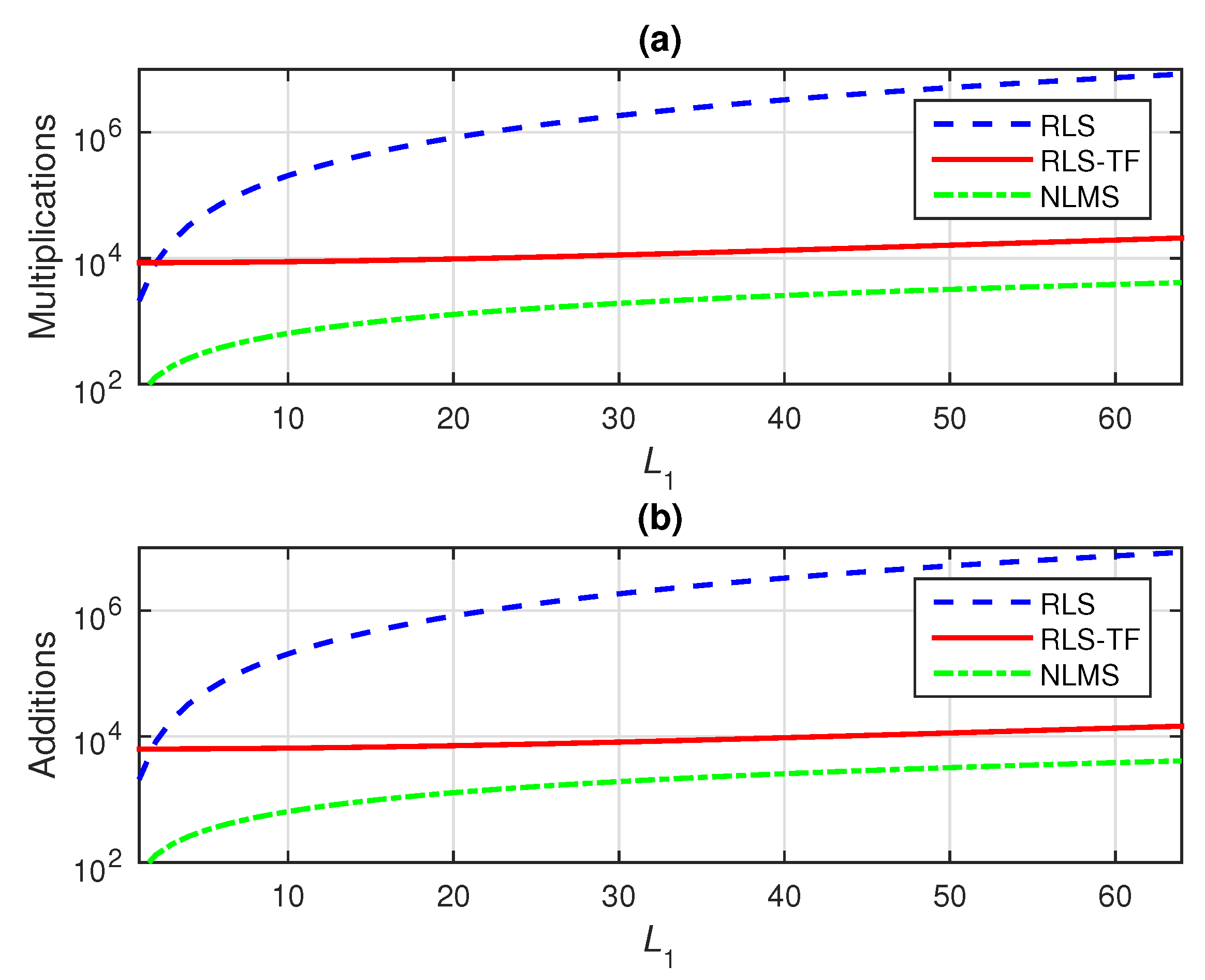
The detailed computational complexities of the proposed RLS-TF algorithm and other benchmark algorithms (i.e., the conventional RLS and NLMS algorithms) are summarized in

Table 2. Computational complexity of the RLS-TF algorithm, as compared to the conventional RLS and NLMS algorithms.

Algorithms	×	+	÷
RLS	$2L^2+2L$	$2L^2+L+1$	1
RLS-TF	$4L+3\left(L_1^2+L_2^2+L_3^2\right)+3\left(L_1+L_2+L_3\right)+\min (L_1,L_2,L_3)$	$3L+2\left(L_1^2+L_2^2+L_3^2\right)+L_1+L_2+L_3+\min (L_1,L_2,L_3)$	3
NLMS	$2L+2$	$2L+3$	1

. For a better visualization, the computational complexities are also illustrated in Figure 1, in terms of the number of multiplications and additions (per iteration), for different values of $L_1$; the other lengths are fixed to $L_2=8$ and $L_3=4$ (similar to the experimental setup from Section 4). As we can notice, the computational complexity of the conventional RLS algorithm was significantly greater, while the computational amount of the proposed RLS-TF algorithm was closer to the conventional NLMS algorithm, especially for higher lengths.

4. Simulation Results

Simulations were performed in the framework of a tensor-based system identification problem, which resulted following the MISO model defined by (12) and (20) and was similar to the setup used in [17]. The input signals that form the third-order tensor $\mathcal{X}\left(n\right)$ are AR(1) processes; they are generated by filtering white Gaussian noises through a first-order system $1/\left(1-0.9z^{-1}\right)$. The additive noise $w\left(n\right)$ is white and Gaussian; its variance was set to ${\sigma }_w^2=0.01$.

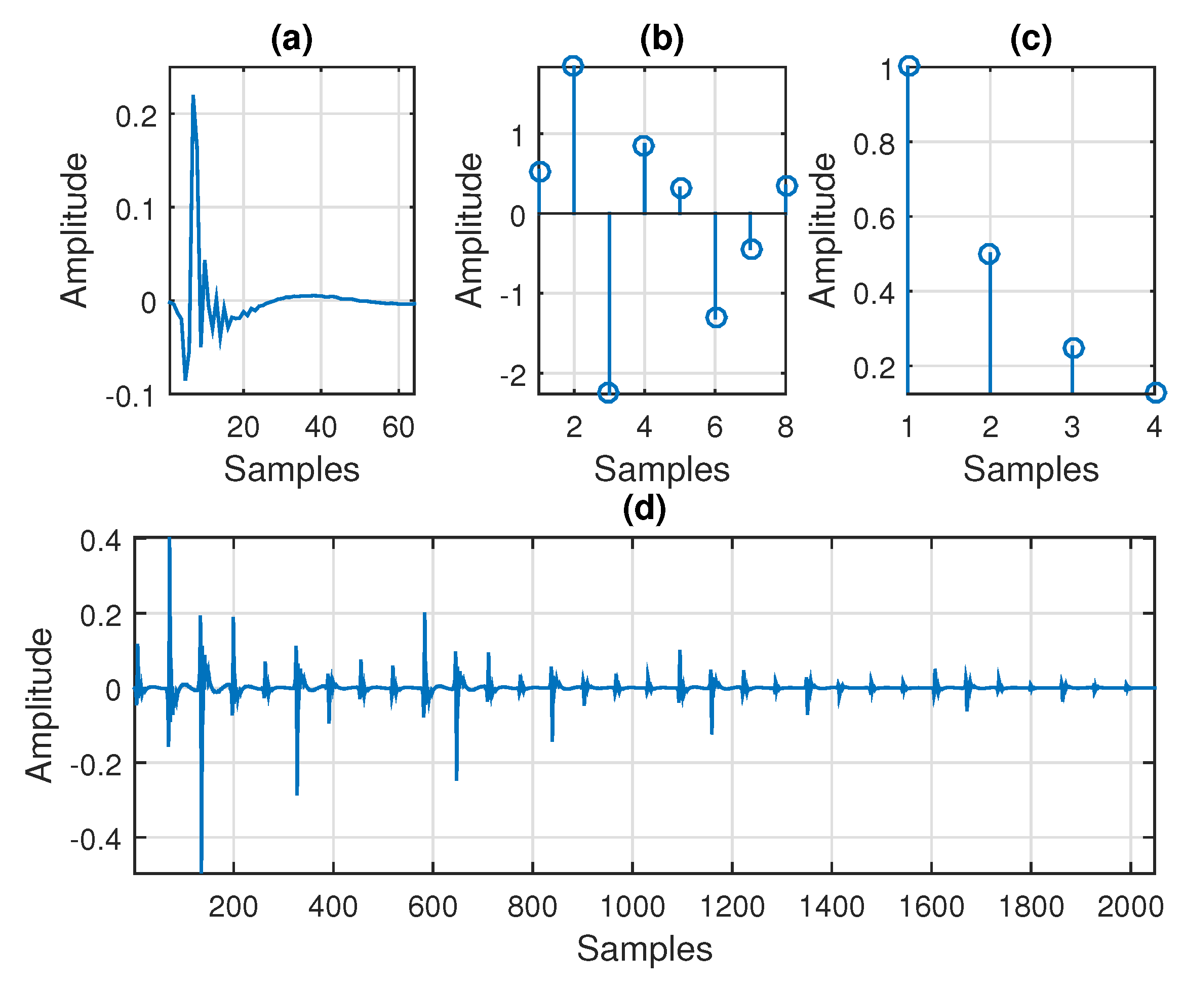
The third-order system used in the simulations and its components (${\mathbf{h}}_1$, ${\mathbf{h}}_2$, and ${\mathbf{h}}_3$) are depicted in Figure 2. First, the component ${\mathbf{h}}_1$ is an impulse response from the G168 Recommendation [26], of length $L_1=64$; it is provided in Figure 2a. Second, in Figure 2b, the component ${\mathbf{h}}_2$ is a random impulse response (with Gaussian distribution) of length $L_2=8$. Third, the coefficients of the last component, i.e., the impulse response ${\mathbf{h}}_3$, are depicted in Figure 2c; those were evaluated as $h_{3,l_3}={0.5}^{l_3-1},l_3=1,2,\dots ,L_3$, using the length $L_3=4$. Therefore, the global impulse response from Figure 2d resulted as $\mathbf{h}={\mathbf{h}}_3\otimes {\mathbf{h}}_2\otimes {\mathbf{h}}_1$, and its length was $L=L_1{L}_2{L}_3=2048$. This global impulse response resembled a channel with echoes, e.g., like an acoustic echo path [27]. Finally, the third-order (rank-1) tensor $\mathcal{H}$ of dimension $L_1\times L_2\times L_3$ could be formed according to (13). In order to test the tracking capabilities of the algorithms, an abrupt change of the system was introduced in the middle of each experiment, by changing the sign of the coefficients of each impulse response.

As shown in Section 3, the proposed RLS-TF algorithm was designed to estimate the individual components of the global system. However, we could identify ${\mathbf{h}}_1$, ${\mathbf{h}}_2$, and ${\mathbf{h}}_3$ up to some scaling factors, as explained using (23). Therefore, to evaluate the identification of these individual impulse responses, a proper performance measure is the normalized projection misalignment (NPM) [28]:

$$\begin{array}{cc}\hfill \mathrm{NPM}\left[{\mathbf{h}}_1,{\widehat{\mathbf{h}}}_1\left(n\right)\right]& =1-{\left[\frac{{\mathbf{h}}_1^T{\widehat{\mathbf{h}}}_1\left(n\right)}{{∥{\mathbf{h}}_1∥}_2{∥{\widehat{\mathbf{h}}}_1\left(n\right)∥}_2}\right]}^2,\hfill \end{array}$$

(55)

$$\begin{array}{cc}\hfill \mathrm{NPM}\left[{\mathbf{h}}_2,{\widehat{\mathbf{h}}}_2\left(n\right)\right]& =1-{\left[\frac{{\mathbf{h}}_2^T{\widehat{\mathbf{h}}}_2\left(n\right)}{{∥{\mathbf{h}}_2∥}_2{∥{\widehat{\mathbf{h}}}_2\left(n\right)∥}_2}\right]}^2,\hfill \end{array}$$

(56)

$$\begin{array}{cc}\hfill \mathrm{NPM}\left[{\mathbf{h}}_3,{\widehat{\mathbf{h}}}_3\left(n\right)\right]& =1-{\left[\frac{{\mathbf{h}}_3^T{\widehat{\mathbf{h}}}_3\left(n\right)}{{∥{\mathbf{h}}_3∥}_2{∥{\widehat{\mathbf{h}}}_3\left(n\right)∥}_2}\right]}^2,\hfill \end{array}$$

(57)

where ${∥·∥}_2$ denotes the Euclidean norm. On the other hand, the global impulse response $\mathbf{h}$ results without any scaling ambiguity. Consequently, we can use a performance measure based on the regular normalized misalignment (NM):

$$\begin{array}{cc}\hfill \mathrm{NM}\left[\mathbf{h},\widehat{\mathbf{h}}\left(n\right)\right]& =\frac{{∥\mathbf{h}-\widehat{\mathbf{h}}\left(n\right)∥}_2^2}{{∥\mathbf{h}∥}_2^2},\hfill \end{array}$$

(58)

which is also equivalent to ${∥\mathcal{H}-\widehat{\mathcal{H}}\left(n\right)∥}_{\mathrm{F}}^2/{∥\mathcal{H}∥}_{\mathrm{F}}^2$, where $\widehat{\mathcal{H}}\left(n\right)={\widehat{\mathbf{h}}}_1\left(n\right)\circ {\widehat{\mathbf{h}}}_2\left(n\right)\circ {\widehat{\mathbf{h}}}_3\left(n\right)$ and ${∥·∥}_{\mathrm{F}}$ denotes the Frobenius norm (the Frobenius norm of a third-order tensor $\mathcal{A}$ is defined as ${∥\mathcal{A}∥}_{\mathrm{F}}=\sqrt{\langle \mathcal{A},\mathcal{A}\rangle }={∥{\mathbf{A}}_{\left[1\right]}∥}_{\mathrm{F}}={∥{\mathbf{A}}_{\left[2\right]}∥}_{\mathrm{F}}={∥{\mathbf{A}}_{\left[3\right]}∥}_{\mathrm{F}}$).

The simulation results should provide answers to several important questions, as follows. (i) What is the influence of the forgetting factors on the performance of the proposed RLS-TF algorithm? (ii) What are the advantages of the RLS-TF algorithm over the previously developed NLMS-TF counterpart [17]? (iii) What are the advantages of the RLS-TF algorithm over the conventional RLS benchmark? The following three experiments are designed to address these issues.

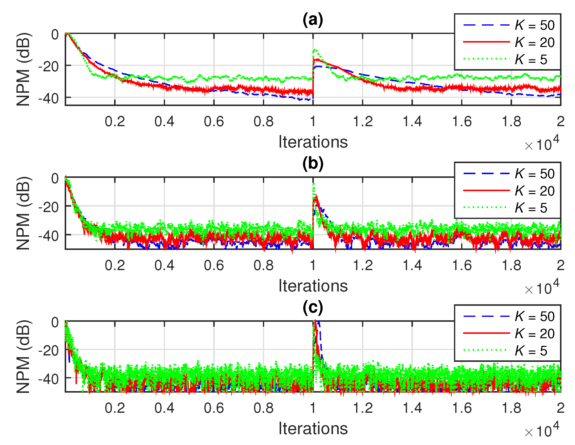
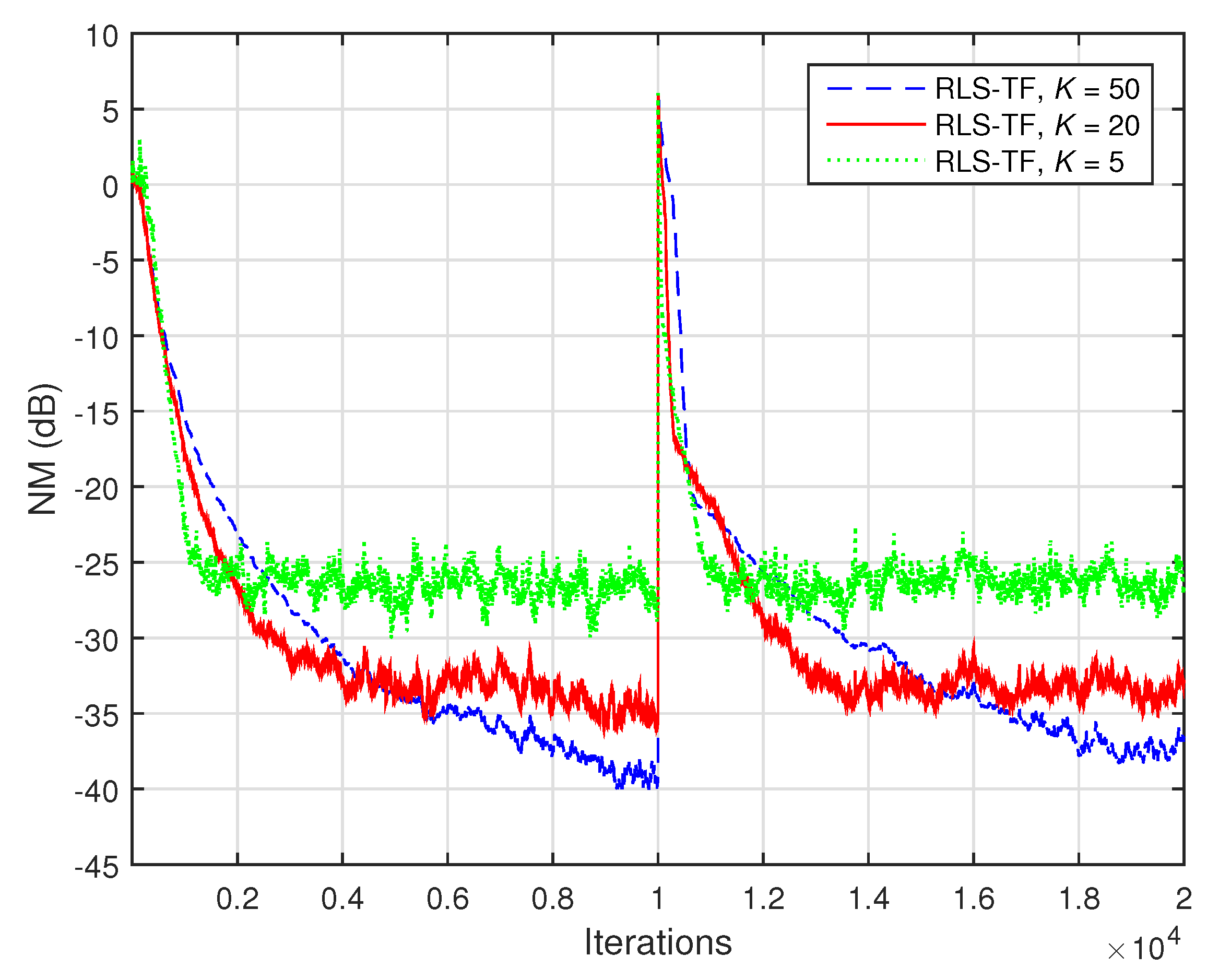
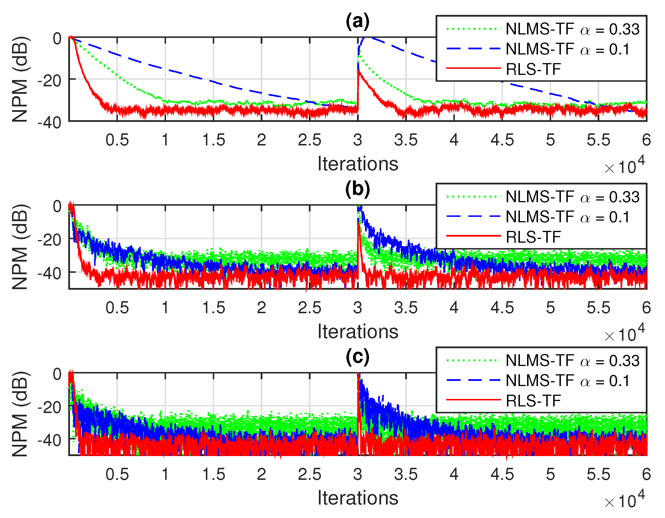
In the first experiment, the performance of the proposed RLS-TF algorithm was analysed with respect to its main parameters, i.e., the forgetting factors ${\lambda }_1$, ${\lambda }_2$, and ${\lambda }_3$. In the case of an RLS-based algorithm, the value of the forgetting factor is usually related to the filter length, following a well-known rule of thumb, as shown in Table 1 (see “Initialization”). In our case, the forgetting factors of the RLS-TF algorithm were set to ${\lambda }_1=1-1/\left(K{L}_1\right)$, ${\lambda }_2=1-1/\left(K{L}_2\right)$, and ${\lambda }_3=1-1/\left(K{L}_3\right)$. As we can notice, the value of each forgetting factor depended on the length of its related filter (i.e., $L_1$, $L_2$, or $L_3$), but also on the constant K. This tuning parameter could be used to adjust the values of the forgetting factors, as indicated in Figure 3 and Figure 4. Clearly, a higher value of K would result in a higher value of the forgetting factor (i.e., closer to one). We could expect that a higher value of the forgetting factor would reduce the misalignment, but slowing down the convergence/tracking [29]. On the other hand, reducing the forgetting factor improves the convergence/tracking, but increasing the misalignment. This behaviour was supported by the results depicted in Figure 3 and Figure 4, in terms of NPM and NM, respectively. As we can notice, the value $K=20$ lead to a good compromise between the performance criteria, so that it would be used in the following experiments.

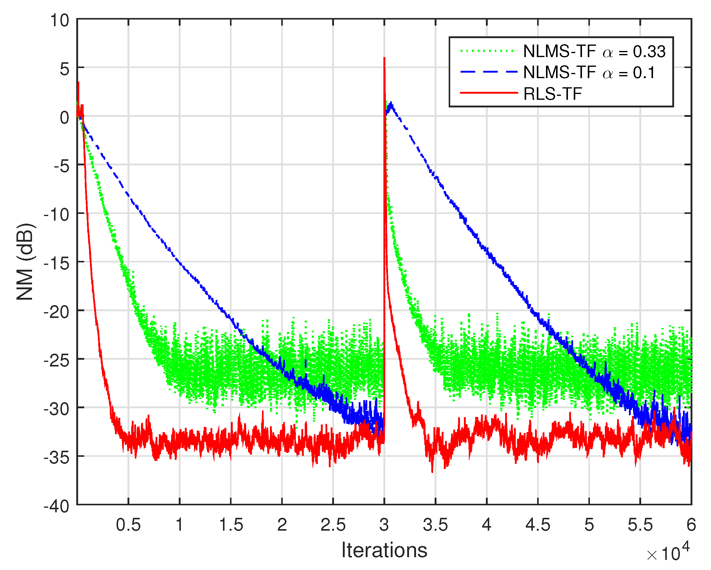
Next, we compare the performance of the proposed RLS-TF algorithm with its previously developed counterpart based on the NLMS algorithm, i.e., NLMS-TF [17]. The overall performance of this algorithm is mainly controlled by its normalized step-sizes, which are positive constants smaller than one. Using notation similar to that involved in [17], we set equal values for these parameters, i.e., ${\alpha }_1={\alpha }_2={\alpha }_3=\alpha$. In the case of the NLMS-TF algorithm, the fastest convergence mode was obtained when ${\alpha }_1+{\alpha }_2+{\alpha }_3\approx 1$, so that we could use $\alpha =0.33$. Smaller values of the normalized step-sizes (e.g., $\alpha =0.1$) reduced the convergence/tracking, but led to a lower misalignment. As shown in Figure 5 and Figure 6 (in terms of NPM and NM, respectively), the RLS-TF algorithm clearly outperformed the NLMS-TF counterpart, achieving a faster convergence rate and tracking, together with low misalignment.

Finally, in the last experiment, we investigated the comparison between the RLS-TF solution and the conventional RLS algorithm. As explained in the last part of Section 3 (related to the computational complexity), the conventional RLS algorithm could also be used for the identification of the global impulse response of length L, based on the cost function from (36). This algorithm uses a single forgetting factor, which can also be set as $\lambda =1-1/\left(KL\right)$, where K is the same tuning constant. The influence of the value of $\lambda$ on the performance of the algorithm is also related to the well-known compromise between low misalignment and fast tracking. In the experiment reported in Figure 7, the conventional RLS algorithm uses two values of the forgetting factor, which were set by varying the tuning constant to $K=1$ and $K=20$. As we can notice, even if the largest value of the forgetting factor (obtained for $K=20$) led to a lower misalignment, the tracking capability of the conventional RLS algorithm was significantly reduced. Clearly, the tracking was improved when using a smaller forgetting factor (corresponding to $K=1$), but the misalignment of the conventional RLS algorithm was much higher in this case. On the other hand, the RLS-TF algorithm outperformed by far its conventional counterpart, in terms of both performance criteria. Moreover, the complexity of the conventional RLS algorithm, i.e., $\mathcal{O}\left(L^2\right)$, was prohibitive for practical implementations, due to the long length of the global filter ($L=2048$). On the other hand, the RLS-TF algorithm worked on the individual components and combined the solutions of three shorter filters, of lengths $L_1$, $L_2$, and $L_3$ (with $L_1{L}_2{L}_3=L$); thus, it was much more computationally efficient. As a trivial example related to the last experiment given in Figure 7, we could mention that the simulation time (using MATLAB) of the RLS-TF algorithm was less than one minute, while the conventional RLS algorithm took hours to reach the final result.

5. Conclusions and Future Works

In this paper, we explored the identification of trilinear forms using the RLS algorithm. The approach was developed in the framework of an MISO system identification problem, based on the decomposition and modelling of third-order tensors. The resulting RLS-TF algorithm was tailored for the identification of such trilinear forms in a more efficient way as compared to the conventional RLS algorithm. Moreover, the proposed RLS-TF algorithm outperformed its previously developed NLMS-TF counterpart in terms of the main performance criteria, providing a faster convergence rate and tracking, together with low misalignment.

The ideas presented in this paper could be further exploited in an extended framework, aiming to identify more general forms of global impulse responses, which cannot be decomposed as rank-1 tensors. Several preliminary results can be found in [30,31,32], but they are applicable only in the bilinear context (i.e., second-order tensors). The extension to the trilinear case represents a very challenging problem, since finding (and approximating) the rank of a higher order tensor is a much more sensitive task. Furthermore, it would be interesting to extend other versions of the NLMS and RLS algorithms (e.g., based on variable step-sizes [33] and variable forgetting factors [34], respectively) to the trilinear forms.

Finally, it would be useful to evaluate how the proposed algorithm could benefit (in terms of implementation) from the current technology of the tensor processing unit (TPU) and the TensorFlow software [35]. This aspect could bring additional advantages, especially in the framework of specific applications related to machine learning/vision, neural networks, and artificial intelligence.

References

1. Comon, P. Tensors: A brief introduction. IEEE Signal Process. Mag. 2014, 31, 44–53. [Google Scholar] [CrossRef] [Green Version]
2. Cichocki, A.; Mandic, D.; De Lathauwer, L.; Zhou, G.; Zhao, Q.; Caiafa, C.; Phan, H.A. Tensor decompositions for signal processing applications: From two-way to multiway component analysis. IEEE Signal Process. Mag. 2015, 32, 145–163. [Google Scholar] [CrossRef] [Green Version]
3. Vervliet, N.; Debals, O.; Sorber, L.; De Lathauwer, L. Breaking the curse of dimensionality using decompositions of incomplete tensors: Tensor-based scientific computing in big data analysis. IEEE Signal Process. Mag. 2014, 31, 71–79. [Google Scholar] [CrossRef]
4. Boussé, M.; Debals, O.; De Lathauwer, L. A tensor-based method for large-scale blind source separation using segmentation. IEEE Trans. Signal Process. 2017, 65, 346–358. [Google Scholar] [CrossRef]
5. Sidiropoulos, N.; De Lathauwer, L.; Fu, X.; Huang, K.; Papalexakis, E.; Faloutsos, C. Tensor decomposition for signal processing and machine learning. IEEE Trans. Signal Process. 2017, 65, 3551–3582. [Google Scholar] [CrossRef]
6. Da Costa, M.N.; Favier, G.; Romano, J.M.T. Tensor modelling of MIMO communication systems with performance analysis and Kronecker receivers. Signal Process. 2018, 145, 304–316. [Google Scholar] [CrossRef] [Green Version]
7. Ribeiro, L.N.; de Almeida, A.L.; Mota, J.C.M. Separable linearly constrained minimum variance beamformers. Signal Process. 2019, 158, 15–25. [Google Scholar] [CrossRef]
8. De Lathauwer, L. Signal Processing Based on Multilinear Algebra. Ph.D. Thesis, Katholieke Universiteit Leuven, Leuven, Belgium, 1997. [Google Scholar]
9. Kolda, T.G.; Bader, B.W. Tensor decompositions and applications. SIAM Rev. 2009, 51, 455–500. [Google Scholar] [CrossRef]
10. Benesty, J.; Paleologu, C.; Ciochină, S. On the identification of bilinear forms with the Wiener filter. IEEE Signal Process. Lett. 2017, 24, 653–657. [Google Scholar] [CrossRef]
11. Paleologu, C.; Benesty, J.; Ciochină, S. Adaptive filtering for the identification of bilinear forms. Digit. Signal Process. 2018, 75, 153–167. [Google Scholar] [CrossRef]
12. Elisei-Iliescu, C.; Stanciu, C.; Paleologu, C.; Benesty, J.; Anghel, C.; Ciochină, S. Efficient recursive least-squares algorithms for the identification of bilinear forms. Digit. Signal Process. 2018, 83, 280–296. [Google Scholar] [CrossRef]
13. Dogariu, L.-M.; Ciochină, S.; Paleologu, C.; Benesty, J. A connection between the Kalman filter and an optimized LMS algorithm for bilinear forms. Algorithms 2018, 11, 211. [Google Scholar] [CrossRef] [Green Version]
14. Ribeiro, L.N.; de Almeida, A.L.F.; Mota, J.C.M. Identification of separable systems using trilinear filtering. In Proceedings of the 2015 IEEE 6th International Workshop on Computational Advances in Multi-Sensor Adaptive Processing (CAMSAP), Cancun, Mexico, 13–16 December 2015; pp. 189–192. [Google Scholar]
15. Rupp, M.; Schwarz, S. A tensor LMS algorithm. In Proceedings of the 2015 IEEE International Conference on Acoustics, Speech and Signal Processing (ICASSP), Brisbane, QLD, Australia, 19–24 April 2015; pp. 3347–3351. [Google Scholar]
16. Dogariu, L.-M.; Ciochină, S.; Benesty, J.; Paleologu, C. An iterative Wiener filter for the identification of trilinear forms. In Proceedings of the 2019 42nd International Conference on Telecommunications and Signal Processing (TSP), Budapest, Hungary, 1–3 July 2019; pp. 88–93. [Google Scholar]
17. Dogariu, L.-M.; Ciochină, S.; Benesty, J.; Paleologu, C. System identification based on tensor decompositions: A trilinear approach. Symmetry 2019, 11, 556. [Google Scholar] [CrossRef] [Green Version]
18. Haykin, S. Adaptive Filter Theory, 4th ed.; Prentice-Hall: Upper Saddle River, NJ, USA, 2002. [Google Scholar]
19. Parathai, P.; Tengtrairat, N.; Woo, W.L.; Gao, B. Single-channel signal separation using spectral basis correlation with sparse nonnegative tensor factorization. Circuits Syst. Signal Process. 2019, 38, 5786–5816. [Google Scholar] [CrossRef]
20. Woo, W.L.; Dlay, S.S.; Al-Tmeme, A.; Gao, B. Reverberant signal separation using optimized complex sparse nonnegative tensor deconvolution on spectral covariance matrix. Digit. Signal Process. 2018, 83, 9–23. [Google Scholar] [CrossRef] [Green Version]
21. Gao, B.; Lu, P.; Woo, W.L.; Tian, G.Y.; Zhu, Y.; Johnston, M. Variational Bayes sub-group adaptive sparse component extraction for diagnostic imaging system. IEEE Trans. Ind. Electron. 2018, 65, 8142–8152. [Google Scholar] [CrossRef]
22. Kiers, H.A.L. Towards a standardized notation and terminology in multiway analysis. J. Chemom. 2000, 14, 105–122. [Google Scholar] [CrossRef]
23. Kroonenberg, P. Applied Multiway Data Analysis; Wiley: Hoboken, NJ, USA, 2008. [Google Scholar]
24. Van Loan, C.F. The ubiquitous Kronecker product. J. Comput. Appl. Math. 2000, 123, 85–100. [Google Scholar] [CrossRef] [Green Version]
25. Bertsekas, D.P. Nonlinear Programming, 2nd ed.; Athena Scientific: Belmont, MA, USA, 1999. [Google Scholar]
26. Digital Network Echo Cancellers; ITU-T Recommendations G.168; ITU: Geneva, Switzerland, 2002.
27. Gay, S.L.; Benesty, J. (Eds.) Acoustic Signal Processing for Telecommunication; Kluwer Academic Publisher: Boston, MA, USA, 2000. [Google Scholar]
28. Morgan, D.R.; Benesty, J.; Sondhi, M.M. On the evaluation of estimated impulse responses. IEEE Signal Process. Lett. 1998, 5, 174–176. [Google Scholar] [CrossRef]
29. Ciochină, S.; Paleologu, C.; Benesty, J.; Enescu, A.A. On the influence of the forgetting factor of the RLS adaptive filter in system identification. In Proceedings of the 2009 International Symposium on Signals, Circuits and Systems, Iasi, Romania, 9–10 July 2009; pp. 205–208. [Google Scholar]
30. Paleologu, C.; Benesty, J.; Ciochină, S. Linear system identification based on a Kronecker product decomposition. IEEE/ACM Trans. Audio Speech Lang. Process. 2018, 26, 1793–1808. [Google Scholar] [CrossRef]
31. Elisei-Iliescu, C.; Paleologu, C.; Benesty, J.; Ciochină, S. A recursive least-squares algorithm based on the nearest Kronecker product decomposition. In Proceedings of the ICASSP 2019—2019 IEEE International Conference on Acoustics, Speech and Signal Processing (ICASSP), Brighton, UK, 12–17 May 2019; pp. 4843–4847. [Google Scholar]
32. Elisei-Iliescu, C.; Paleologu, C.; Benesty, J.; Stanciu, C.; Anghel, C.; Ciochină, S. Recursive least-squares algorithms for the identification of low-rank systems. IEEE/ACM Trans. Audio Speech Lang. Process. 2019, 27, 903–918. [Google Scholar] [CrossRef]
33. Benesty, J.; Rey, H.; Rey Vega, L.; Tressens, S. A non-parametric VSS NLMS algorithm. IEEE Signal Process. Lett. 2006, 13, 581–584. [Google Scholar] [CrossRef]
34. Paleologu, C.; Benesty, J.; Ciochină, S. A robust variable forgetting factor recursive least-squares algorithm for system identification. IEEE Signal Process. Lett. 2008, 15, 597–600. [Google Scholar] [CrossRef]
35. Jouppi, N.P.; Young, C.; Patil, N.; Patterson, D.; Agrawal, G.; Bajwa, R.; Bates, S.; Bhatia, S.; Boden, N.; Borchers, A.; et al. In-datacenter performance analysis of a tensor processing unit. In Proceedings of the 44th Annual International Symposium on Computer Architecture, Toronto, ON, Canada, 24–28 June 2017; pp. 1–12. [Google Scholar]
Figure 1. Computational complexity of the proposed RLS-TF algorithm, as compared to the conventional RLS and NLMS algorithms, as a function of L 1 ; the other dimensions are set to L 2 = 8 and L 3 = 4 : (a) number of multiplications per iteration and (b) number of additions per iteration.
Algorithms 13 00135 g001
Figure 2. The components of the third-order system used in simulations: (a) h 1 is the first impulse response (of length L 1 = 64 ) from the G168 Recommendation [26]; (b) h 2 is a randomly generated impulse response (of length L 2 = 8 ), with Gaussian distribution; (c) the impulse response h 3 (of length L 3 = 4 ), with the coefficients computed as h 3 , l 3 = 0.5 l 3 1 , with l 3 = 1 , 2 , , L 3 ; and (d) the global impulse response (of length L = L 1 L 2 L 3 = 2048 ) results based on (17), h = h 3 h 2 h 1 .
Algorithms 13 00135 g002
Figure 3. Normalized projection misalignment (NPM) evaluated based on (55)–(57), in dB, for the identification of the individual impulse responses from Figure 2a–c, using the RLS-TF algorithm with different values of the forgetting factors λ i = 1 1 / ( K L i ) , i = 1 , 2 , 3 (varying the value of K): (a) NPM h 1 , h ^ 1 ( n ) , (b) NPM h 2 , h ^ 2 ( n ) , and (c) NPM h 3 , h ^ 3 ( n ) .
Algorithms 13 00135 g003
Figure 4. Normalized misalignment (NM) evaluated based on (58), in dB, for the identification of the global impulse response h (of length L = 2048 ) from Figure 2d, using the RLS-TF algorithm with different values of the forgetting factors λ i = 1 1 / ( K L i ) , i = 1 , 2 , 3 (varying the value of K).
Algorithms 13 00135 g004
Figure 5. Normalized projection misalignment (NPM) evaluated based on (55)–(57), in dB, for the identification of the individual impulse responses from Figure 2a–c, using the NLMS-TF algorithm [17] (with different normalized step-sizes α 1 = α 2 = α 3 = α ) and the RLS-TF algorithm (with the forgetting factors λ i = 1 1 / ( K L i ) , i = 1 , 2 , 3 , where K = 20 ): (a) NPM h 1 , h ^ 1 ( n ) , (b) NPM h 2 , h ^ 2 ( n ) , and (c) NPM h 3 , h ^ 3 ( n ) .
Algorithms 13 00135 g005
Figure 6. Normalized misalignment (NM) evaluated based on (58), in dB, for the identification of the global impulse response h (of length L = 2048 ) from Figure 2d, using the NLMS-TF algorithm [17] (with different normalized step-sizes α 1 = α 2 = α 3 = α ) and the RLS-TF algorithm (with the forgetting factors λ i = 1 1 / ( K L i ) , i = 1 , 2 , 3 , where K = 20 ).
Algorithms 13 00135 g006
Figure 7. Normalized misalignment (NM) evaluated based on (58), in dB, for the identification of the global impulse response h (of length L = 2048 ) from Figure 2d, using the conventional RLS algorithm (with different values of the forgetting factor λ = 1 1 / ( K L ) , varying the value of K) and the RLS-TF algorithm (with the forgetting factors λ i = 1 1 / ( K L i ) , i = 1 , 2 , 3 , where K = 20 ).
Algorithms 13 00135 g007