Late Acceptance Hill-Climbing Matheuristic for the General Lot Sizing and Scheduling Problem with Rich Constraints

Abstract

This paper considers the general lot sizing and scheduling problem with rich constraints exemplified by means of rework and lifetime constraints for defective items (GLSP-RP), which finds numerous applications in industrial settings, for example, the food processing industry and the pharmaceutical industry. To address this problem, we propose the Late Acceptance Hill-climbing Matheuristic (LAHCM) as a novel solution framework that exploits and integrates the late acceptance hill climbing algorithm and exact approaches for speeding up the solution process in comparison to solving the problem by means of a general solver. The computational results show the benefits of incorporating exact approaches within the LAHCM template leading to high-quality solutions within short computational times.

1. Introduction

In many production processes, a fraction of the manufactured products can be defective due to an unreliable production system. Often, defective items incorporate substantial value and it is possible to rework them into an “as-good-as-new” state. Incorporating this feature results in a more ecological friendly production process as disposal reduces. Furthermore, reworking of defective items can only take place within a specific time span. For instance, in the pharmaceutical industry rework often has to take place in a short amount of time due to likely increasing contamination. In this context, we formulate a related problem and address a model formulation of the general lot sizing and scheduling problem with rework termed as GLSP-RP, which was first presented by [1]. This problem also considers lifetime constraints for defective items. As the authors report, the GLSP-RP model is hardly solvable by a general-purpose solver in an adequate amount of time. Even for small problem instances of non-practical size, it requires more than 1800 s. This leads to the necessity of faster approaches providing solutions within reasonable execution times.

Matheuristics can be defined as those solution approaches obtained from the interoperation between metaheuristics and mathematical programming techniques [2]. Within matheuristics, decomposition approaches belong to one of the most relevant algorithms (some recent examples can be consulted in, for example, [3,4,5]). For instance, the principal idea behind proposing the matheuristic version of POPMUSIC is to decompose the problems into smaller (and likely more tractable) ones and solve them by means of an exact technique [6]. As remarked by [7] to successfully apply decomposition matheuristic approaches, one may develop an iterated procedure where the information is interchanged along the process. Adapting those ideas to well-known single point metaheuristics such as late acceptance hill-climbing (LAHC, [8]) permits, within a hill-climbing framework, to substitute the inherent method for generating candidate solutions by an exact method solving a given sub-problem. Furthermore, recently, [9] showed by means of the unrelated parallel machine scheduling problem the importance of including advanced local search methods to improve the solution quality in LAHC. This, thus, led to our research question about how LAHC would perform if we use an exact approach instead of a local search solver.

Based on the previous discussion, the contribution of this paper is twofold:

• We investigate the relationship between the original formulation of the general lot sizing and scheduling problem (GLSP) and the GLSP-RP by providing a comprehensive discussion of both problems.
• For solving the GLSP-RP, we propose the Late Acceptance Hill-climbing Matheuristic (LAHCM) as a general solution framework, which is inspired by and integrates the LAHC strategy with the exact approaches, i.e., the solution of optimization models for reduced problems configured in the spirit of the LAHC. To assess its performance, we evaluate it over a set of well-defined instances. The computational results indicate that by means of our approach we are able to improve the objective function values for several instances where a general-purpose solver such as CPLEX (https://www.ibm.com/nl-en/analytics/cplex-optimizer) is not able to find optimal solutions in the given time limit of 1800 s.

The outline of this paper is as follows. In Section 2, those works related to the GLSP as well as its respective formulation are discussed. The general lot sizing and scheduling problem considering rework and lifetime constraints for defective items is explained in Section 3. Later, our matheuristic solution approach based on late acceptance hill-climbing is described in Section 4. The extensive computational experience is reported in Section 5. Finally, some conclusions and further research lines are exposed in Section 6.

2. Literature Review

To jointly decide on lot sizing and scheduling has attracted many researchers in recent years producing a rich body of literature on different models and problem formulations including, for example, the general lot sizing and scheduling problem (GLSP). In this paper, we present a novel solution approach for an extended version of the GLSP and focus on this specific problem while referring to [10], and [11] for extensive literature reviews on different simultaneous lot sizing and scheduling problems. In Section 2.1, we reappraise the original model formulation of the GLSP as it will later be used in the algorithm for creating an initial solution. In Section 2.2, we review solution approaches and model extensions to the GLSP.

2.1. The General Lot Sizing and Scheduling Problem

The GLSP was originally introduced by [12]. The authors presented two versions of the model, namely the GLSP-CS (Conservation of Setup state) where the setup state is preserved over idle periods and the GLSP-LS (Loss of Setup state). In this section, with the aim of making the paper self-contained, we present an extended mixed-integer programming (MIP) formulation for the GLSP-CS that includes sequence-dependent setup times as presented by [13] and a revised version of the minimum lot size constraint introduced by [14] and use the name GLSP for this formulation in the further course of this paper. The GLSP features integrated production planning and scheduling for capacitated single facility environments with multiple products. The setups for these products are sequence-dependent in times and costs, implying that setting up the production of the products in a certain sequence can be more favorable than another in terms of time and costs; see also [15,16]. To simultaneously determine the production sequence and the quantity of production lots, the GLSP includes a two-level time structure. Products $j=1,\dots ,J$ are scheduled over a finite planning horizon consisting of macro-periods $t=1,\dots ,T$ with given length. Micro-periods $m=1,\dots ,L_T$ (with $L_T$ denoting the last micro-period of the last macro-period T) are used to model the production sequence of products within the macro-periods. Each macro-period t consists of a predefined non-overlapping sequence of micro-periods with $|M_t|$ being an advance fixed total number of micro-periods within a macro-period t. The length of each macro-period is given by the input parameter for the resource capacity $b_t$; the lengths of micro-periods are decision variables expressed by the number of productions in the micro-period. A production lot consists of a sequence of consecutive micro-periods where the same product is produced and may continue over a series of micro-periods and macro-periods. As described, this model presents an extended version of the GLSP-CS where the setup state is preserved over idle periods, i.e., if after an idle micro-period the same product is produced as before, no additional setup is necessary.

The objective is to find an optimal production quantity and a sequence that minimizes overall production costs, consisting of setup changeover and inventory-holding costs.

Table 1. Variables, parameters and indices used in the model.

Indices
$i,j$	Products with $i,j=1,\dots ,J$
$L_t$	Denoting the last micro-period of a macro-period t
m	Micro-periods $m=1,\dots ,L_T$ with $L_T={\sum }_{t=1}^T\left|M_t\right|$
$M_t$	Set of micro-periods m within macro-period t
t	Macro-periods with $t=1,\dots ,T$
Parameters
$b_t$	Available capacity in macro-period t in time units
$d_{j,t}$	Demand of product j in period t
$f_{i,j}$	Sequence-dependent setup costs for a change over from product i to j
$h_j$	Inventory holding cost factor for product j
${\kappa }_j$	Minimum lot size amount of product j
$|M_t|$	Fixed number of micro-periods within a macro-period t
$s{t}_{i,j}$	setup times for a change over from product i to j
$t{p}_j$	Process time per unit of product j
M	big number, e.g., $max{\left(b\right)}_{t\in T}$
Variables
$s_{j,t}$	Inventory of product j in period t
$x_{j,m}$	Binary setup variable, 1 if product j is set up for production
	in micro-period m, 0 otherwise
$y_{j,m}$	Production amount of product j in micro-period m
$z_{i,j,m}$	Changeover variable, 1 if production is changed from product i to j
	in micro-period m, 0 otherwise

presents the variables, parameters and indices of the GLSP model.

The problem is formulated as follows:

$$min\sum _{j=1}^J\sum _{t=1}^T{h}_j·s_{j,t}+\sum _{i=1}^J\sum _{j=1}^J\sum _{m=1}^{L_T}{f}_{i,j}·z_{i,j,m}$$

(1)

$$s_{j,t-1}+\sum _{m\in M_t}{y}_{j,m}-d_{j,t}=s_{j,t}\forall j,t$$

(2)

$$\sum _{j=1}^J\sum _{m\in M_t}t{p}_j·y_{j,m}\le b_t-\sum _{i,j=1}^J\sum _{m\in M_t}s{t}_{i,j}·z_{i,j,m}\forall t,i\ne j$$

(3)

$$y_{j,m}\le M·x_{j,m}\forall j,m$$

(4)

$$\sum _{j=1}^J{x}_{j,m}=1\forall m$$

(5)

$$y_{j,m}\ge {\kappa }_j(x_{j,m}-x_{j,m-1})\forall j,t,m\ne L_t$$

(6)

$$y_{j,m}+y_{j,m+1}\ge {\kappa }_j(x_{j,m}-x_{j,m-1})\forall j,t,m=L_t$$

(7)

$$z_{i,j,m}\ge (x_{i,m-1}+x_{j,m})-1\forall i,j,m,i\ne j$$

(8)

$$y_{j,m},s_{j,t},z_{i,j,m}\ge 0\forall j,m,t$$

(9)

$$x_{j,m}\in \{0,1\}\forall j,m$$

(10)

The objective Function (1) minimizes the overall costs consisting of the holding costs for produced items and the sequence-dependent setup costs. Equation (2) depicts the inventory balancing constraint. It states that the inventory in macro-period t is composed of the inventory of the previous macro-period $t-1$, the production amount of all micro-periods belonging to t subtracted by the demand of period t. Inequality (3) states that the maximum available capacity ($b_t$) of macro-period t reduced by the sum of sequence-dependent setup times incurred by setup changes from product i to product j with $m\in M_t$ must be greater or equal to the sum of processing times in all micro-periods belonging to macro-period t. Constraints (4) and (5) ensure that product j can only be produced in micro-period m, if a setup for product j is performed in m, i.e., if the binary setup variable ($x_{j,m}$) is set to one and that only a single product can be produced at a time in a micro-period m. The authors of [12] pointed out that minimum lot sizes have to be included, otherwise wrong calculations of setup costs could occur as a result of setup state changes without product changes in cases where the setup cost matrix does not satisfy the triangle inequality (i.e., $f_{i,k}+f_{k,j}\ge f_{ij}$ with $i,j,k\in 1,\dots ,J$). As shown by [14], this originally introduced minimum lot size constraint was strictly limited as a production state between two consecutive periods; it is only conserved if the available capacity exceeds the minimum production quantity. Therefore, the authors adjusted Constraint (6) and introduced Constraint (7) to enforce the production continuity across macro-periods. Constraint (8) presents the changeover logic and Constraints (9) and (10) enforce non-negative and binary variables, respectively.

Many researchers have worked on this specific model and developed extensions, solution approaches, and applications for industrial settings, which will be reviewed in the next section.

2.2. Solution Approaches and Model Extensions

The authors of [12] present a solution procedure for the GLSP-based on the local search algorithm threshold accepting. The procedure starts from a configuration defined by a fixed setup pattern and calculates the corresponding lot sizes and costs through backward oriented heuristics. New candidates are created by neighborhood operations that change the old configuration and are accepted as a new configuration if they provide an improved solution. To escape local optima, new candidates are also accepted if their solution quality is not worse than a specific threshold, while the convergence of the algorithm is ensured by lowering this threshold. In [13,17], an improved version of this procedure is used that determines lot sizes optimally for a fixed pattern through ”dual reoptimization” instead of heuristically for solving two extended versions of the GLSP, i.e., the GLSP with setup times and the GLSP for parallel lines, respectively. While this approach proves to be efficient for the single-line GLSP, the results of the multi-line formulation are insufficient. Therefore, Meyr and Mann (2013) adjust the approach by aggregating the original multi-line ”master-problem” in order to decompose it into a set of isolated single-line ”sub-problems”, which are solved by the heuristic provided in [13]. A model extension of the single-stage GLSP to multiple production stages is presented in [18]. The authors of [19] adjust this model with respect to the synchronization of the machines and present several reformulations of the problem based on variable redefinitions. In addition, three heuristic approaches are presented to solve the problem. In [20], the authors present a GLSP-based model formulation called the synchronized and integrated two-level lot sizing and scheduling problem (SITLSP), which is motivated by industrial settings, mainly of soft-drink companies where the production process involves two interdependent levels with decisions concerning raw material storage and soft drink bottling. The authors of [21] solve the SITLSP by a genetic algorithm (GA) and study single-population and multi-population approaches. Additional solution approaches for the SITLSP are studied by [22]. They apply a tabu search (TS), threshold accepting (TA), genetic algorithm (GA) and hybrid genetic algorithms using a combination of GA with TS and TA, respectively, to the problem. The authors observe that for the hybrid approaches, an execution of TA and TS over the best individual of each population results in high computational times and that a strategy where these strategies are only executed when the best individual of all populations is updated performs best. The authors of [23] propose a multi-population GA with individuals structured in ternary trees to solve data provided by a soft-drink company. A simplified model formulation of the SITLSP called two-stage multi-machine lot scheduling model (P2SMM) is proposed by [24] where each filling line can only be connected to a single tank at the same point in time. As a relaxation approach, they first solve a single-stage version of the model and afterward determine the setup variables of the P2SMM. In addition, they propose fix-and-relax strategies and combinations of them with a relaxation approach to solve the P2SMM. Reference [25] study different relax-and-fix strategies to solve a model formulation similar to the single-stage P2SMM with only one production line and the production bottleneck in the bottling stage. Reference [26] propose four different alternative single-stage formulations of the P2SMM where the first two are based on the single-stage GLSP model with sequence-dependent setup times and costs, while the other two are asymmetric traveling salesman problem (ATSP)-based formulations with different subtour elimination constraints. Numerical experiments show that solution strategies based on the ATSP formulations perform best for the P2SMM. The authors of [27] apply a combined genetic algorithm and mathematical programming approach to solve the P2SMM that outperforms the approaches presented in [26]. In [28], the authors adjust the P2SMM for an application in the brewery industry and solve the problem heuristically by using a constructive relax-and-fix heuristic and several improvement procedures based on fix-and-optimize strategies. Note that these approaches borrow ideas from the much older POPMUSIC approach of [29].

The authors of [30] present a GLSP-based model formulation for a multi-product multi-level job shop production where they subdivide the macro-periods into three types of micro-periods: one type for production, one for setups, and one for idle time. Due to the high complexity of their formulation, only problems with a small number of periods, products, and machines can be solved to optimality. In [31], the authors propose a formulation for lot sizing and scheduling in a flow shop environment with sequence-dependent setups and develop four fix-and-relax heuristics that rely on successive resolutions of reduced size MIP-formulations of the problem. The authors of [32] propose a formulation based on the model of [30] for a flexible flow shop environment with sequence-dependent setups. Additionally, the authors of [33] develop two algorithms based on a rolling horizon approach where first, all binary variables of the problem are relaxed. Then, relaxed binary variables of the current period are divided into the two groups so that the members of the first and second groups get value one or zero, respectively.

The authors of [34] present two MIP-formulations for joint lot sizing and scheduling motivated by an animal feed plant. While the first formulation sequences each period independently, the second model takes linking setup states between periods into account. The authors present three relax-and-fix (RF) heuristic approaches where they either apply the RF heuristic for relaxing and fixing the lot sizes or the periods. While the RF heuristic on the integer lot sizes performs best, the authors observed that a forward-oriented RF over the periods acts like a greedy heuristic resulting occasionally in infeasible solutions for instances known to be feasible. In [35], the author presents an extended formulation for the GLSP with multiple production stages where an embedded State-Task-Network is used to model product substitution and flexible Bill-of-Materials by introducing several tasks that produce the same product while using different input products. In [36], the authors consider a GLSP-based model with different machine configurations. Therefore, the authors introduce tools as an additional, capacitated resource in a single-stage, multi-machine problem and model tool changeovers instead of product changeovers. As a specific tool cannot be used on more than one machine at a time, continuous variables for the starting and ending times of tool use are introduced. The authors of [37] present a hybrid mixed-binary model based on the GLSP for a practical problem of the process industry and propose two transportation-based reformulations, namely the quantity-based transportation problem (QTP) and the proportional transportation problem (PTP). In their statistical analysis, they observe that the PTP reformulation performs best on average, but for cases of a high level of minimum production quantities, it is outperformed by the QTP reformulation. In [38], the authors propose three novel mathematical formulations for a two-stage GLSP where multiple products are produced on parallel, non-identical machines inspired by the textile industry and solve them with a MIP-solver. The authors of [39] adapt this model for usage in the yarn production and solve the problem by means of a hybrid method called hamming-oriented partition search, which is a branch-and-bound-based procedure that incorporates a fix-and-optimize improvement method.

In [40], the authors propose a GLSP-based model for a pulp and paper mill planning problem and solve the problem with a two-step approach with a MIP-based construction heuristic followed by a MIP-based improvement heuristic. The authors of [41] extend this model to the multi-stage scenario and include additional constraints with the objective to maximize the steam output used to generate electrical energy. To solve the problem, the authors develop a hybrid approach that combines the general variable neighborhood search heuristic, a specific heuristic called speeds constraint heuristic and an exact solver. In [42], the authors also extend the model of [40] to the case of parallel non-identical paper machines and solve the problem by a hybrid solution method composed of an exact method embedded in a genetic algorithm. The authors of [43] present a model formulation for a production environment with wear and tear of resources and maintenance activities based on a combination of the PLSP and the GLSP where exogenous macro-periods with given length and demand are combined with endogenous micro-periods of flexible length. The authors propose a fix-and-optimize type decomposition heuristic to solve this problem.

The authors of [44] present a GLSP formulation with multiple machines in a job shop environment and solve the problem with two MIP-based algorithms based on the rolling horizon iterative procedure. A multi-stage GLSP formulation for a flexible job-shop problem is presented by [45] and solved with a metaheuristic method that combines a GA with particle swarm optimization (PSO) and a local search heuristic. Deterioration and perishability for the GLSP are considered by [46]. The authors propose a model formulation that includes products that deteriorate after a maximum lifetime while being stored in an inventory. In this paper, we regard a model formulation based on this GLSP version, which was first presented by [1] and combines lifetime constraints for defective items with the ideas of an imperfect production process and rework, called GLSP-RP.

Reference [47] study a robust optimization and a scenario-based two-stage stochastic programming model for the General Lot-Sizing and Scheduling Problem (GLSP) under demand uncertainty. The authors propose an extensive simulation experiment based on Monte Carlo to evaluate different characteristics of the solutions, such as average costs, worst-case costs, and standard deviation. The authors of [48] focus on a general lot-sizing and scheduling problem, including perishable food products, and apply two mixed-integer programming based heuristics to the problem. The authors use relax-and-fix approaches as a constructive heuristic to find an initial feasible solution and afterward apply a fix-and-optimize heuristic to improve the obtained initial solution.

3. The GLSP with Rework and Lifetime Constraint for Defective Items

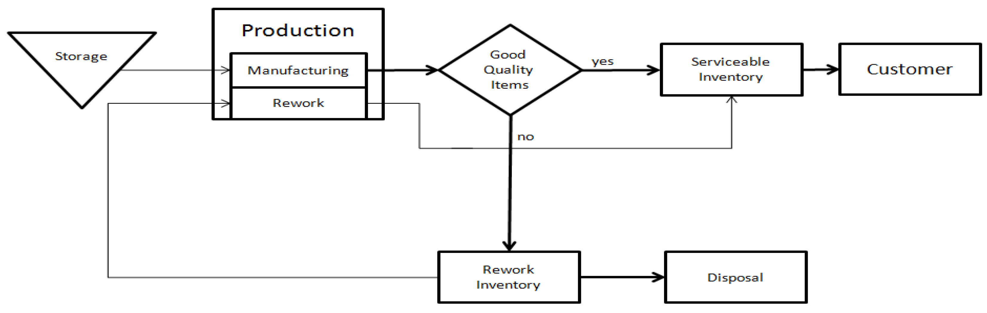
The GLSP-RP was introduced by [1] to model process environments where conflicting items are required to avoid contact as they are subject to contamination, for example, the food processing industry where an-allergenic food items are produced on the same machine as regular food items. The problem considers an imperfect production system where a fraction of the planned lot size is not of serviceable quality and goes to a separate rework inventory where it is stored till it is reworked and shipped to customers or disposed of, which is illustrated in Figure 1.

Note that, in this paper, no distinction will be made between the quality of good quality items and reworked items. Furthermore, we assume that the rework process always succeeds. For scheduling rework lots, a joint setup variable is considered, i.e., if the machine is set up for the original production in micro-period m (i.e., $x_{j,m}=1$) and followed by a rework lot for product j in $m+1$ and vice versa, no additional setup is needed and, therefore, no additional setup costs occur. To address this in the model, the binary setup variable $x_{j,m}$ of the GLSP formulation is redefined as the binary joint setup-variable. In addition, the defectives have a fixed lifetime while being stored in the rework inventory, i.e., if the defective items are not reworked in a fixed time frame expressed by a number of consecutive micro-periods (${\Omega }_j$) they become scrap and have to be disposed, resulting in disposal costs (${\lambda }_j$).

Table 2. Additional variables and parameters for the general lot sizing and scheduling problem with defective items and lifetime constraints (GLSP-RP).

Parameters
$h_j^R$	Inventory holding cost factor for defective items of product j
${\lambda }_j$	Disposal cost for one perished item of product j
${\Omega }_j$	Lifetime of product j in micro-periods
${\Theta }_{j,t}$	Proportion of defective items $0\le {\Theta }_{j,t}<1$ of product j in t
$t{p}_j^R$	Process time for reworking a defective item per unit of product j
Variables
$R_{j,m}$	Number of defective items of product j produced in micro-period m
$s_{j,m}^D$	Number of perished items of rework inventory of product j
	in micro-period m
$s_{j,m}^R$	Number of defective items stored in rework inventory of product j
	in micro-period m
$x_{j,m}$	Binary joint-setup variable, 1 if product j is set up for production and/or rework
	in micro-period m, 0 otherwise
$y_{j,m}^R$	Quantity of defective items of product j reworked in micro-period m
$y_{j,m}^S$	Production amount of good-quality items of product j in micro-period m

shows the additional variables and parameters of the GLSP-RP.

The GLSP-RP is formulated as follows:

$$\begin{array}{r}min\sum _{j=1}^J\sum _{t=1}^T{h}_j·s_{j,t}+\sum _{i=1}^J\sum _{j=1}^J\sum _{m=1}^{L_T}{f}_{i,j}·z_{i,j,m}+\sum _{j=1}^J\sum _{m=1}^{L_T}{h}_j^R·s_{j,m}^R\\ +\sum _{j=1}^J\sum _{m=1}^{L_T}{\lambda }_j·s_{j,m}^D+\sum _{j=1}^J{\lambda }_j·(s_{j,L_T}^R+R_{j,L_T})\end{array}$$

(11)

$$y_{j,m}^S=\lfloor [y_{j,m}·(1-{\Theta }_{j,t})]\rfloor \forall j,t,m\in M_t$$

(12)

$$R_{j,m}=\lceil (y_{j,m}·{\Theta }_{j,t})\rceil \forall j,t,m\in M_t$$

(13)

$$s_{j,t-1}+\sum _{m\in M_t}{y}_{j,m}^S+\sum _{m\in M_t}{y}_{j,m}^R-d_{j,t}=s_{j,t}\forall j,t$$

(14)

$$s_{j,m-1}^R+R_{j,m}-y_{j,m}^R-s_{j,m}^D=s_{j,m}^R\forall j,m$$

(15)

$$s_{j,m}^D\ge \sum _{\tau =1}^{m-{\Omega }_j}{R}_{j,\tau }-\sum _{\tau =1}^{m-1}{y}_{j,\tau }^R-\sum _{\tau =1}^{m-1}{s}_{j,\tau }^D\forall j,m$$

(16)

$$\sum _{\tau =1}^{m-1}{R}_{j,\tau }-\sum _{\tau =1}^{m-1}{y}_{j,\tau }^R\ge y_{j,m}^R\forall j,m$$

(17)

$$\sum _{j=1}^J\sum _{m\in M_t}(t{p}_j·y_{j,m}+t{p}_j^R·y_{j,m}^R)\le b_t-\sum _{i,j=1}^J\sum _{m\in M_t}s{t}_{i,j}·z_{i,j,m}\forall t\in M_t,i\ne j$$

(18)

$$y_{j,m}+y_{j,m}^R\le M·x_{j,m}\forall j,m$$

(19)

$$\sum _{j=1}^J{x}_{j,m}=1\forall m$$

(20)

$$y_{j,m}+y_{j,m}^R\ge {\kappa }_j(x_{j,m}-x_{j,m-1})\forall j,t,m\ne L_t$$

(21)

$$y_{j,m}+y_{j,m+1}+y_{j,m}^R+y_{j,m+1}^R\ge {\kappa }_j(x_{j,m}-x_{j,m-1})\forall j,t,m=L_t$$

(22)

$$z_{i,j,m}\ge (x_{i,m-1}+x_{j,m})-1\forall i,j,m,i\ne j$$

(23)

$$y_{j,m},y_{j,m}^R,y_{j,m}^S,s_{j,t},s_{j,t}^R,R_{j,m},z_{i,j,m},s_{j,m}^D\ge 0\forall j,m,t$$

(24)

$$x_{j,m}\in \{0,1\}\forall j,m$$

(25)

The adjusted objective Function (11) of the GLSP-RP additionally considers the holding costs of defective items and the disposal costs for defective items that perished while holding. As a positive rework inventory at the end of the planning horizon is allowed for feasibility reasons any positive amount of defectives stored in the rework inventory or incurred in the last micro-period of the planning horizon ($m_{j,m}=L_T$) has to be disposed, leading to disposal costs that are included in the last term of the objective function. Equations (12) and (13) present the production process of defectives as described in [49]. Concerning the planned lot size amount $y_{j,m}$ of a given micro-period m, only the reduced amount of $y_{j,m}^S$ is of serviceable quality and can be used for demand satisfaction. The amount of items that are defective ($R_{j,m}$) has to be stored in the rework inventory and later reworked or disposed. Consequently, the GLSP-RP regards two separate inventories for serviceable items and defective items. Equation (14) shows the amended inventory balancing constraint for serviceable items. The serviceable inventory in macro-period t is composed of the inventory of the previous period $t-1$, the amount of serviceable and rework production in all micro-periods belonging to macro-period t subtracted by the demand of period t. Equation (15) considers the rework inventory. The rework inventory is micro-period based as it symbolizes an interim inventory for the defective items. It is composed of the rework inventory in $m-1$, the number of defective items of micro-period m minus the reworked items in m and the number of items that passed their lifetime while being stored ($s_{j,m}^D$). The interrelation between storage time and lifetime of the defective items is shown in Equation (16). It states that the amount of spoiled defectives for a given micro-period m is calculated by the defectives produced by the original production process from the beginning of the planning horizon until micro-period m deduced by the lifetime length ${\Omega }_j$ of the defectives, less those items that are already reworked until micro-period $m-1$ and defectives that were already disposed in previous micro-periods. Constraint (17) ensures that defectives of micro-period $m-1$ can be reworked in m the earliest. The capacity constraints given in Inequalities (18) show that in addition to the sum of the processing times for the original production, the rework production process also has to be taken into account. Consequently, it has the maximum available capacity ($b_t$) of macro-period t minus the sum of sequence dependent setup times by setup changes from product i to product j not to be exceeded by the total sum of processing times for the original and the rework production occurring in micro-periods belonging to t. Equation (19) depicts the joint setup constraint. This constraint ensures that product j can only be produced or reworked, respectively, in micro-period m, if a setup for product j is performed in m, with $UB$ symbolizing a large number that has to be chosen in a way that it does not restrict the production volume. Constraint (20) ensures that only a single product is produced and/or reworked in micro-period m. Constraints (21) and (22) are the adjusted minimum lot size constraints and ensure that after a setup change the minimum lot size amount (${\kappa }_j$) has to be fulfilled by production and/or rework. Constraint (22) enforces the production continuity across macro-periods as described by [14], i.e., if the time interval of the last micro-period of a macro-period t is not sufficient to produce or rework ${\kappa }_j$, and production is continued in the next macro-period ($t+1$), then the sum of production and rework of micro-period m and $m+1$ has to satisfy the minimum production quantity. Constraint (23) presents the changeover logic and enforces variables ($z_{i,j,m})$ for micro-period m to equal one if product i is produced or reworked in micro-period $m-1$ and followed by a production or rework lot of another product j in micro-period m. Constraints (24) and (25) enforce non-negative and binary variables, respectively.

4. Late Acceptance Hill-Climbing Matheuristic Template

The late acceptance hill-climbing (LAHC) algorithm is a single-point iterative search algorithm proposed by [8] that accepts non-improving movements when the objective function value of a candidate has a better value than the one number of iterations before. Namely, while in the standard hill-climbing algorithm a candidate solution is compared to the direct predecessor, in LAHC the candidate is compared with the current solution several iterations before.

LAHC has been successfully applied to several optimization problems. In the following, some of them are briefly reviewed. The authors of [8] apply the LAHC to exam timetabling problems reporting a competitive performance. This problem is later addressed by [50] where they present a hybridization of an adaptive artificial bee colony (ABC) and LAHC. The latter is applied as a local search procedure during the exploitation of the ABC algorithm. The results indicate that this hybridization performs better than other modifications of the ABC algorithm. In [51], the authors apply the LAHC to the traveling purchaser problem showing a suitable performance for solving that problem. The authors of [52] use this algorithm for balancing two-sided assembly lines with multiple constraints. The LAHC, in this case, is able to provide the same solutions as those provided by the optimization model implemented using LINGO for the small-sized instances. For large-sized instances, the model is not able to provide an optimal solution in reasonable computational time, thus leaving LAHC the best option for those instances. The author of [53] applies LAHC to the liner shipping fleet reposition problem. The author compares it to simulated annealing (SA) reporting that LAHC performs well on small instances, but on larger instances, SA exhibits better performance. The authors of [54] experimentally examine their proposed method and compare it to search techniques that employ a cooling schedule, i.e., simulated annealing, threshold accepting and the great deluge algorithm for the traveling salesman problem. In [55], the authors present a cutoff time strategy based on the coupon collector’s problem and apply it to the LAHC algorithm. The authors tested that approach on the Travelling Salesman Problem, the Quadratic Assignment Problem, and the Permutation Flow-shop Scheduling Problem. Their results show that the proposed strategy is a valid stopping method for a one-point stochastic local search algorithm that accepts worsening moves. The authors of [56] apply the LAHC for finding train composition causing greatest fatigue damage in railway bridges. In [9], the authors propose an LAHC approach to solve the unrelated parallel machine scheduling problem with sequence and machine-dependent setup times, the reported results indicated the relevancy of including advanced local search methods to improve LAHC performance. This raises the research question related to using an exact solver instead of a local search within LAHC.

Based on the previous discussion, there are two reasons for developing and proposing the Late Acceptance Hill-Climbing Matheuristic (LAHCM) in this paper. First, the LAHC as a metaheuristic reportedly performs well for the traveling purchaser problem and the traveling salesman problem. The traveling purchaser problem incorporates a choice option regarding the inclusion of nodes. As including rework into dynamic lot sizing shows a high similarity to this property and lot sizing models are frequently formulated as traveling salesman based formulations including the GLSP (see [26]), it is worth examining the application of LAHC for solving our GLSP model formulation. Second, considering the relevant performance of this strategy in the related literature and the benefits of exact approaches in terms of solution quality, the interplay between the two types of approaches is considered in LAHCM. In this sense, exact approaches are exploited to solve subproblems optimally and generate candidate solutions within LAHC. To the best of our knowledge, this is the first LAHC matheuristic template proposed so far and, therefore, we are contributing in this paper by presenting a LAHCM as a general solution framework.

The pseudo-code of LAHCM considering the GLSP-RP is reported in Algorithm 1. The parameter of the algorithm is a list length parameter l, which establishes the number of solutions to be stored. The initialization of the algorithm consists of creating an initial solution for the problem instance p (line 1). The current best solution is set to the initial solution (line 2), the number of iterations and the array for storing the solutions collected in the last l iterations are initialized in lines 3-6. The LAHCM search procedure is depicted in lines 7–15 and executed until a given stopping criterion is met. The index of the solution from l iterations before is stored in v (line 8). A candidate solution $s^{\prime }$ is generated by solving a subproblem by means of an exact method (fixandsolve ()) defined by the user (line 9). At this point, it should be noted that the main difference between a standard LAHC and LAHCM resides in the way the candidate solution is generated. Furthermore, if the candidate solution enhances the objective value of the current solution or the one from l iterations before, then the candidate solution is the new current solution (lines 10–11). Moreover, the candidate solution is compared to the best solution found so far $s_{best}$ in order to check if the candidate solutions improve the best one and thus replace it (lines 12–13). Finally, the solution is stored in the solution array and the iteration counter is incremented. In LAHCM, the search process is stopped when no improvement is obtained by means of the performance comparison shown in line 10.

As can be seen, the LAHCM template does not require a neighborhood structure to generate candidate solutions but an exact approach permitting to optimally generate candidate solutions for its mathematical programming neighborhood that can be defined by fixing some parameters or reducing the instance at hand. The previous permits, because of the size reduction, solving the subproblems with exact approaches in reasonable times to optimality.

4.1. Initial Solution

In order to generate an initial solution for the LAHCM algorithm, the procedure createinitialsol () (see Algorithm 1) is proposed. Its functioning consists of relaxing the problem by not considering the constraints concerning the rework and lifetime for defective items, that is to say, we solve the GLSP (see Section 2.1). Once that problem is solved, the solution is appropriately entered by means of fixing the sequence variables $x_{j,m}$ of the GLSP-RP. That is done by extending its corresponding model (Section 3) with the following constraints:

$$x_{j,m}\ge x{\left(GLSP\right)}_{j,m}\forall j,m$$

(26)

where $x{\left(GLSP\right)}_{j,m}$ denote the variable values taken in the GLSP solution.

Algorithm 1: Matheuristic Late Acceptance Hill-Climbing algorithm (LAHCM)

By means of this procedure, an initial solution is obtained in a reasonable computational time. It is worth pointing out that the solution entered to the GLSP-RP optimization model (Section 3) has the binary setup variables fixed. Since the initial solution comes from the GLSP, the selection of the variables is performed without losing the sense of feasibility. With the goal of facilitating the understanding of the initial solution generation process, an illustrative example considering three products ($j=1,\dots ,3$), three macro-periods ($t=1,\dots ,3$), and a fixed number of five micro-periods ($M_t=5$) per macro-period is presented. The available capacity for all macro-periods is constant with $b_t=400$. For all products, the processing times per product are $t{p}_j=1$, the holding costs are $h_j=5$, and the minimum lot size amount is ${\kappa }_j=10$. The other parameters of this example are set as follows:

$f_{i,j}$ = $\left[\begin{array}{ccc}0& 0.25& 10\\ 0.25& 0& 5\\ 10& 5& 0\end{array}\right]$ $s{t}_{i,j}$ = $\left[\begin{array}{ccc}0& 0.5& 5\\ 0.5& 0& 2\\ 5& 2& 0\end{array}\right]$ $d_{j,t}$ = $\left[\begin{array}{ccc}95& 91& 108\\ 0& 238& 58\\ 107& 150& 93\end{array}\right]$

The first step for generating an initial solution is to solve the corresponding GLSP. This way, for the above-mentioned example the optimal solution is reported in

Table 3. GLSP optimal solution.

GLSP	t:	1						2						3
	m:	1	2	3	4	5		6	7	8	9	10		11	12	13	14	15
	j = 1	1	0	0	0	0		0	0	0	0	1		1	1	1	0	0
$x_{j,m}$	j = 2	0	1	0	0	0		0	0	0	1	0		0	0	0	1	0
	j = 3	0	0	1	1	1		1	1	1	0	0		0	0	0	0	1
	j = 1	96	0	0	0	0		0	0	0	0	90		0	0	108	0	0
$y_{j,m}$	j = 2	0	79	0	0	0		0	0	0	159	0		0	0	0	58	0
	j = 3	0	0	113	0	0		0	144	0	0	0		0	0	0	0	93
	j = 1	1						0						0
$s_{j,t}$	j = 2	79						0						0
	j = 2	6						0						0

. It should be noted that since the values of variables $s_{j,t}$ correspond to macro-periods, to avoid repetition only one number is reported for each row/block.

In the solution, we observe six setup changes with a total of 15.75 in setup changing costs. As the available capacity in $t=2$ with $b_t=400$ is not sufficient to produce the total demand for all three products in $t=2$, proportions of the demand of products $j=1$ and $j=2$ are produced and stored in $t=1$ leading to storage costs, of 410. Therefore, the overall cost for the GLSP solution is 425.75.

As previously described, additional parameters are needed for the GLSP-RP. Consequently, the lifetime of defective items while stored in the rework inventory is set to three micro-periods for all products (${\Omega }_{j,m}=3$) and the disposal cost is ${\lambda }_j=1000$ per item. Regarding rework, we include rework holding costs of $h_j^R=1$, rework processing costs of $t{p}_j^R=1$ for all j. The fraction of defectives per product and macro-period is given as follows:

$${\Theta }_{j,t}=\left[\begin{array}{ccc}0& 0.005& 0.01\\ 0.005& 0.01& 0.02\\ 0& 0& 0.005\end{array}\right]$$

The solution for the GLSP-RP with the fixed setup sequence is shown in

Table 4. Fixed GLSP-RP CPLEX solution.

GLSP-RP	t:	1						2						3
	m:	1	2	3	4	5		6	7	8	9	10		11	12	13	14	15
	j = 1	1	0	0	0	0		0	0	0	0	1		1	1	1	0	0
$x_{j,m}$	j = 2	0	1	0	0	0		0	0	0	1	0		0	0	0	1	0
	j = 3	0	0	1	1	1		1	1	1	0	0		0	0	0	0	1
	j = 1	137	0	0	0	0		0	0	0	0	50		107	0	0	0	0
$y_{j,m}$	j = 2	0	149	0	0	0		0	0	0	100	0		0	0	0	50	0
	j = 3	0	0	10	97	0		243	0	0	0	0		0	0	0	0	0
	j = 1	137	0	0	0	0		0	0	0	0	49		105	0	0	0	0
$y_{j,m}^S$	j = 2	0	148	0	0	0		0	0	0	99	0		0	0	0	49	0
	j = 3	0	0	10	97	0		243	0	0	0	0		0	0	0	0	0
	j = 1	0	0	0	0	0		0	0	0	0	1		2	0	0	0	0
$R_{j,m}$	j = 2	0	1	0	0	0		0	0	0	1	0		0	0	0	1	0
	j = 3	0	0	0	0	0		0	0	0	0	0		0	0	0	0	0
	j = 1	0	0	0	0	0		0	0	0	0	0		1	2	0	0	0
$y_{j,m}^R$	j = 2	0	0	0	0	0		0	0	0	0	0		0	0	0	0	0
	j = 3	0	0	0	0	0		0	0	0	0	0		0	0	0	0	0
	j = 1	0	0	0	0	0		0	0	0	0	0		0	0	0	0	0
$s_{j,m}^D$	j = 2	0	1	0	0	0		0	0	0	1	0		0	0	0	1	0
	j = 3	0	0	0	0	0		0	0	0	0	0		0	0	0	0	0
	j = 1	0	0	0	0	0		0	0	0	0	1		2	0	0	0	0
$s_{j,m}^R$	j = 2	0	0	0	0	0		0	0	0	0	0		0	0	0	0	0
	j = 3	0	0	0	0	0		0	0	0	0	0		0	0	0	0	0
	j = 1	42						0						0
$s_{j,t}$	j = 2	148						9						0
	j = 2	0						93						0

. As in Table 3, variables $s_{j,t}$ only report for each row/block one value as they correspond to macro-periods.

The above solution is used as the starting solution for solving the GLSP-RP with the LAHCM approach. Its objective function value is 4478.75. As can be checked, the setup costs of 15.75 for the GLSP-RP are the same as for the GLSP due to the same setup sequence. The imperfect production process results in much higher storage costs with 1460 costs for the inventory storage and an additional three costs for the rework inventory. The greatest cost driver by far are the disposal costs. As a result of the fixed production sequence, not all defective items can be reworked in a timely manner and therefore disposal costs of 3000 occur.

4.2. Mathematical Programming-Based Neighborhood

As discussed in the previous section, LAHCM differentiates from the standard LAHC in the way the candidate solutions are generated. While in the LAHC a neighborhood structure is usually used, in LAHCM generation of the candidate solution is done by means of an exact algorithm. Thus, in order to produce a candidate solution for the GLSP-RP, the method fixandsolve () is proposed. By means of this function, an input solution is used for extracting and fixing decision variables with the aim of generating smaller sub-problems and solving them in an exact way, producing thus a candidate solution. In a similar way as proposed in [6] through the definition of reduced sub-problems from larger and more complex ones, we are able to address them using an exact algorithm in a small and reasonable computational time. This, as discussed in the relevant section, allows improving the quality of the provided solution while reducing the overall solving time. The input of our approach considers different strategies in order to obtain a reduced sub-problem. In the current work, we use the following strategies:

• Strategy 1 (${\alpha }_1$): The $x_{j,m}$ variables are fixed except for those regarding a product j selected at random.
• Strategy 2 (${\alpha }_2$):The $x_{j,m}$ variables are fixed except for those regarding two products j and $j^{\prime }$ selected at random and where $j\ne j^{\prime }$.
• Strategy 3 (${\alpha }_3$):The $x_{j,m}$ variables are fixed except for those regarding three products j, $j^{{}^{\prime }}$, and $j^{{}^{″}}$ selected at random and where $j\ne j^{{}^{\prime }}\ne j^{{}^{″}}$.

Henceforth, the resulting subset of non-fixed variables of $x_{j,m}$ is denoted as $x_{j,m}^f$. Moreover, the application of these strategies requires previous information about those variables that are to be fixed. That is done by considering previous information from a given solution s.

The pseudo-code of fixandsolve () is depicted in Algorithm 2. For a given problem instance of the GLSP-RP, the algorithm fixes some of the decisions associated to the variables x taking into account an input solution s. To determine the subset of variables to be free from x (i.e., $x^f$), a strategy is selected at random (line 2). Afterward, the optimization model of the GLSP-RP is solved for the ensuing sub-problem obtained from the input instance p with the decisions concerning x fixed except for $x^f$ (line 3). Hence, the model to be solved includes the following:

$$x_{j,m}^f\ge 0,\forall j,m.$$

(27)

The solution $s^{\prime }$ obtained from solving the reduced problem is compared to the input one to check if an improvement has been achieved (line 4). If no improvement is achieved, the input solution s is returned (line 7).

Algorithm 2: Fix and Solve algorithm for the GLSP-RP

4.3. Illustrative Example of the Functioning of the LAHCM for the GLSP-RP

With the goal of facilitating the comprehension of LAHCM, this subsection presents an example case of its functioning using the problem instance provided in Section 4.1 and considering a list length (l) of two.

Initial Solution: As detailed in Section 4.1, for creating a starting solution, the production sequence of the GLSP is given to the GLSP-RP, i.e., the complete sequence of $x_{j,m}$ of the GLSP is given to the GLSP-RP with no rescheduling enabled.

Table 5. Production sequence of the initial solution for the GLSP-RP.

GLSP	t:	1						2						3
	m:	1	2	3	4	5		6	7	8	9	10		11	12	13	14	15
	j = 1	1	0	0	0	0		0	0	0	0	1		1	1	1	0	0
$x{\left(initial\right)}_{j,m}$	j = 2	0	1	0	0	0		0	0	0	1	0		0	0	0	1	0
	j = 3	0	0	1	1	1		1	1	1	0	0		0	0	0	0	1

shows that the resulting sequence of the initial GLSP-RP solution matches the sequence of the GLSP.

The objective function value of the initial solution (i.e., 4478.75) is stored in the list $l=\left[4478.75\right]$ and the iterative procedure with relaxation of the sequence is started.

Iteration 1: The strategy selected at random is ${\alpha }_2$ and the selected products within the strategy are $j=1$ and 2.

Therefore, the binary setup variables for $j=1$ and 2 are reset to zero for all micro-periods m, which is once exemplified in

Table 6. Relaxed production sequence of the initial solution for the GLSP-RP.

GLSP	t:	1						2						3
	m:	1	2	3	4	5		6	7	8	9	10		11	12	13	14	15
	j = 1	0	0	0	0	0		0	0	0	0	0		0	0	0	0	0
$x{\left(relaxed\right)}_{j,m}$	j = 2	0	0	0	0	0		0	0	0	0	0		0	0	0	0	0
	j = 3	0	0	1	1	1		1	1	1	0	0		0	0	0	0	1

. This allows a rescheduling of the sequence of products 1 and 2.

The above sequence is given to the GLSP-RP, producing thus a reduced problem, which is solved by means of an exact algorithm. The optimal solution of this problem results in the following new production sequence for iteration 1:

Having the sequence of products $j=1$ and $j=2$ free while the remaining products are fixed leads to four rescheduling decisions (shown in bold in

Table 7. Output production sequence of Iteration 1 for the GLSP-RP.

GLSP-RP	t:	1						2						3
	m:	1	2	3	4	5		6	7	8	9	10		11	12	13	14	15
	j = 1	1	1	0	0	0		0	0	0	0	0		0	1	1	0	0
$x{\left(iteratio{n}_1\right)}_{j,m}$	j = 2	0	0	0	0	0		0	0	0	1	1		1	0	0	0	0
	j = 3	0	0	1	1	1		1	1	1	0	0		0	0	0	1	1

) and results in an objective function value of 998.25. This new solution does not include disposal costs. Moreover, this objective value is added to the list $l=[4478.75;998.25]$ and the updated production sequence will be the new input sequence for iteration 2. As the list is filled (with the predefined list length $l=2$), the next solutions of the next iterations will be compared to the first entry of the list until the stopping criterion is met.

Iteration 2: The strategy selected at random is ${\alpha }_1$ and the selected product within the strategy is $j=1$.

All values of the production sequence of iteration 1 are fixed except for product $j=1$. This is given as an input to the GLSP-RP. This reduced problem does not lead to any rescheduling and, therefore, results in the same objective function value of 998.25, which is lower than the first entry of the list (i.e., $998.25<4478.75$). Consequently, the first entry of the list is dropped and the objective function value of iteration 2 is added: $l=[998.25;998.25]$.

Iteration 3: The strategy selected at random is ${\alpha }_1$ and the selected product within the strategy is $j=3$. In this iteration of the algorithm, the products’ sequence is fixed except for product $j=3$. The optimal solution of the resulting reduced problem leads to a solution for the GLSP-RP with two rescheduling decisions, which are shown in

Table 8. Production sequence of Iteration 3 for the GLSP-RP.

GLSP-RP	t:	1						2						3
	m:	1	2	3	4	5		6	7	8	9	10		11	12	13	14	15
	j = 1	1	1	0	0	0		0	0	0	0	0		0	1	1	0	0
$x{\left(iteratio{n}_3\right)}_{j,m}$	j = 2	0	0	1	1	0		0	0	0	1	1		1	0	0	0	0
	j = 3	0	0	0	0	1		1	1	1	0	0		0	0	0	1	1

.

The new objective function value is 994.25, which is lower than the corresponding entry of the list (i.e., $994.25<998.25$). Therefore, that entry of the list is dropped and the objective function value of iteration 2 is added to the end of the list: $l=[998.25;994.25]$.

Iteration 4: The strategy selected at random is ${\alpha }_1$ and the selected product within the strategy is $j=2$.

All values of the production sequence of iteration 3 are fixed except for product $j=2$. Having the decision concerning this product free does not lead to any improvement and thus the objective function value of 994.25 is maintained. Nevertheless, this objective function value is lower than the corresponding one of the list (i.e., $994.25<998.25$). Therefore, the entry of the list is dropped and the objective function value of iteration 4 is added to the end of the list: $l=[994.25;994.25]$.

Iteration 5: The strategy selected at random is ${\alpha }_2$ and the selected products within the strategy are $j=1$ and 3.

Having the setup sequence of product $j=2$ fixed and those with respect to products $j=1$ and $j=3$ unfixed does not enable any improving rescheduling, this results thus in the same objective function value of 994.25. This value is compared to the corresponding entry list. As both values are the same, the stopping criterion is met and the method ends with the final objective value of 994.25.

5. Computational Results

In this section, we provide a numerical analysis of the algorithm. We compare the algorithm to benchmark results for data classes that are generated with the same methodology as in [1], which is explained in more detail in the next section. The algorithm is programmed in JAVA and CPLEX 12.6 is used as the standard MIP-solver for solving the MIP formulations of the GLSP and iteratively the GLSP-RP with updated production sequences. CPLEX is is a high-performance general-purpose solver commonly used for solving linear and mixed-integer programming problems. All experiments are conducted on a computer equipped with an Intel Core i5-24510M CPU with 2.3 GHz and 6 GB RAM. We will present the parameters for the data classes in Section 5.1, and afterward, we will present the solutions of the algorithm and compare them to the CPLEX results in Section 5.2.

5.1. Data Set

All data classes consist of 50 instances. For generating the data classes we followed the same methodology as described in [1]. While the authors focused on a sensitivity analysis by varying specific parameters and test them for different numbers of micro-periods within the macro-periods we are going to test the performance of our algorithm for a single number of $M_t$ per class. We build three different data classes (A, B and C) where class A has the highest number of periodic decisions (i.e., 4 macro-periods and 7 micro-periods within a macro-period) and is therefore supposed to be the hardest class to solve.

Table 9. Parameter settings for the data classes.

Parameter	Class A	Class B	Class C
# of instances	50	50	50
# of products (j)	5	4	6
# of macro-periods (t)	4	3	2
# of micro-periods within t ($|M_t|$)	7	6	8
$d_{j,t}$	[0;40,120]	[0;40,120]	[0;600,1000]
$f_{i,j}$	[100,400]	[100,400]	[100,400]
$s{t}_{i,j}$	$f_{i,j}$/10	$f_{i,j}$/10	[10,40]
$t{p}_j$	1	1	1
$t{p}_j^R$	0.5	0.5	0.75
$h_j$	[10,20]	[10,20]	[1,5]
$h_j^R$	$h_j$/$|M_t|$	$h_j$/$|M_t|$	($h_j$/$|M_t|$)*0.75
${\kappa }_j$	10	10	50
${\lambda }_j$	1000	1000	1000
${\Omega }_j$	3	3	2
${\Theta }_{j,t}$	[0;0.005,0.03]	[0;0.005,0.03]	[0;0.005,0.03]
$b_t$	${\sum }_{j=1}^J{\sum }_{t=1}^T{d}_{j,t}\ast 2$	${\sum }_{j=1}^J{\sum }_{t=1}^T{d}_{j,t}\ast 2$	${\sum }_{j=1}^J{\sum }_{t=1}^T{d}_{j,t}\ast 0.6$

summarizes the parameter settings for all data classes.

5.2. Algorithm Results

For testing our algorithm, we set a 100 s time limit on every iteration and a global time limit of 1800 s and compared the results to the best found solution by CPLEX 12.6 in a time limit of 1800 s. Concerning the algorithm parameters, we analyzed its performance for three relaxation strategies, i.e., ${\alpha }_1,{\alpha }_2$ and ${\alpha }_3$ (see Section 4.2), respectively, and tested the algorithm with regards to its main parameter l, i.e., for $l=1,10,20$, and 50. The results for all instances of the three data classes are shown in

Table 10. Results of class A.

Class A		CPLEX			LAHCM ($\mathit{l}=1$)				LAHCM ($\mathit{l}=10$)				LAHCM ($\mathit{l}=20$)				LAHCM ($\mathit{l}=50$)
Instance		Objective	Time		Objective	Time	Iterations		Objective	Time	Iterations		Objective	Time	Iterations		Objective	Time	Iterations
1		6049.71	1800 s		15535.14	106 s	5		5749.71	568 s	37		5749.71	548 s	52		5799.71	665 s	69
2		6099.29	1800 s		11273.29	101 s	3		6646.57	229 s	27		5392.71	255 s	50		5443.85	508 s	88
3		4597.86	1800 s		9076.71	241 s	8		3902.43	204 s	13		3902.43	208 s	29		4295.85	800 s	120
4		10941.60	1800 s		8799.86	235 s	4		8477.86	922 s	38		8318.14	1128 s	57		8088.00	1558 s	94
5		6332.86	1800 s		14586.85	119 s	4		5803.00	407 s	36		5733.50	655 s	45		5715.71	849 s	57
6		7872.14	1800 s		7422.14	121 s	4		7372.14	322 s	19		7372.14	622 s	46		7249.28	1172 s	76
7		5074.14	1800 s		14331.85	102 s	7		5363.71	286 s	30		4875.57	280 s	39		4674.14	543 s	65
8		7044.71	1800 s		10723.57	125 s	7		6157.85	293 s	34		7118.43	407 s	39		6367.85	669 s	86
9		7846.14	1800 s		9596.28	116 s	5		8243.28	722 s	31		8048.57	619 s	28		7763.42	1434 s	112
10		5972.00	1800 s		6290.29	239 s	11		5884.85	605 s	39		6032.57	452 s	45		5884.85	935 s	86
11		5030.00	1800 s		6050.71	137 s	5		4780.00	529 s	44		4685.71	501 s	35		4529.42	543 s	78
12		4625.00	1800 s		4628.28	144 s	9		4297.28	251 s	32		4347.29	304 s	41		4185.57	316 s	74
13		5176.00	1800 s		5909.57	168 s	7		4179.85	263 s	18		3925.71	364 s	44		3957.71	389 s	65
14		6927.00	1800 s		7077.00	289 s	12		7043.29	318 s	13		6526.99	280 s	27		6327.00	450 s	54
15		5316.14	1800 s		5450.43	137 s	6		5252.85	321 s	22		4966.14	343 s	34		5152.85	408 s	61
16		7428.86	1800 s		8962.29	160 s	10		6831.43	376 s	20		7167.00	1085 s	70		6627.71	764 s	84
17		5168.00	1800 s		10950.85	103 s	4		5178.00	385 s	17		4878.00	376 s	47		4859.14	705 s	71
18		4793.71	1800 s		8443.43	105 s	4		4019.86	293 s	21		4069.85	362 s	56		4119.85	330 s	75
19		6122.14	1800 s		7208.71	409 s	7		5606.57	721 s	42		6222.14	590 s	33		5318.85	1714 s	105
20		6858.00	1800 s		9694.43	120 s	5		6396.29	669 s	61		6096.71	548 s	49		6061.28	946 s	91
21		5355.57	1800 s		8035.28	114 s	3		5455.57	530 s	36		5455.57	259 s	59		5455.57	1066 s	105
22		5983.86	1800 s		6472.57	118 s	6		6026.14	229 s	24		5477.71	615 s	49		5477.71	612 s	72
23		7784.29	1800 s		14793.29	141 s	5		6427.71	875 s	33		6384.28	979 s	71		6876.14	965 s	98
24		4834.86	1800 s		5756.00	131 s	4		4913.71	156 s	23		5325.71	344 s	42		4715.14	652 s	76
25		7774.29	1800 s		7876.29	146 s	3		7086.29	272 s	18		7186.29	223 s	27		7230.57	1040 s	59
26		4199.57	1800 s		7983.57	106 s	4		3674.43	226 s	31		3854.43	260 s	39		3656.42	443 s	87
27		6020.71	1800 s		9443.57	127 s	3		5218.00	170 s	28		5370.71	466 s	55		5218.00	1031 s	121
28		6260.29	1800 s		7497.14	133 s	4		5775.43	234 s	20		6956.29	298 s	24		5624.28	512 s	70
29		9204.29	1800 s		8537.71	134 s	8		7157.14	705 s	36		7157.14	809 s	57		7157.14	1542 s	122
30		3922.71	1800 s		4428.43	113 s	7		3572.71	172 s	24		3572.71	229 s	36		3572.71	528 s	61
31		7513.14	1800 s		15084.29	102 s	3		5958.00	403 s	34		5770.00	649 s	47		5770.00	1800 s	115
32		6869.14	1800 s		7081.57	259 s	7		6673.43	253 s	21		6233.28	1210 s	59		6137.14	1157 s	84
33		4902.71	1800 s		8331.71	142 s	4		4502.14	306 s	29		4502.14	671 s	71		4704.42	1110 s	110
34		5602.86	1800 s		9533.86	133 s	4		5488.57	316 s	30		5638.57	598 s	24		5576.14	904 s	61
35		8134.57	1800 s		13257.86	202 s	5		6821.86	700 s	37		6571.85	706 s	42		6571.85	1589 s	111
36		3811.86	1800 s		5019.71	164 s	7		3667.29	208 s	33		3720.71	244 s	31		3517.29	363 s	72
37		6487.71	1800 s		8290.29	131 s	7		6637.29	410 s	32		6588.71	477 s	38		6637.28	1037 s	74
38		8037.43	1800 s		9030.29	179 s	3		6831.14	533 s	21		6831.14	827 s	57		6831.14	1345 s	62
39		7095.43	1800 s		7939.00	131 s	4		6696.29	272 s	27		6053.71	593 s	50		5928.85	653 s	72
40		4176.00	1800 s		9561.14	107 s	5		4226.00	202 s	28		4274.29	237 s	48		4174.28	538 s	98
41		4141.71	1800 s		4058.57	139 s	4		3974.29	170 s	15		4031.43	173 s	31		3931.43	453 s	81
42		4625.00	1800 s		7156.71	103 s	5		5435.00	145 s	17		4337.43	585 s	71		4437.43	839 s	91
43		9968.57	1800 s		9535.99	602 s	9		8421.99	604 s	49		8622.00	701 s	38		8542.14	1333 s	81
44		4851.29	1800 s		9972.42	105 s	5		4497.14	263 s	27		4669.14	406 s	31		4597.14	449 s	64
45		5191.14	1800 s		10550.71	101 s	4		3649.57	184 s	20		3599.57	250 s	25		3601.71	474 s	92
46		7982.71	1800 s		14014.29	101 s	3		7749.57	510 s	19		6879.29	629 s	45		7059.28	1304 s	89
47		7434.43	1800 s		8172.43	131 s	4		6610.43	313 s	26		6214.00	514 s	30		6490.42	865 s	57
48		8093.57	1800 s		8817.57	139 s	4		8958.99	266 s	48		7449.14	490 s	34		6791.85	1423 s	83
49		6721.14	1800 s		6426.29	140 s	7		6304.29	325 s	21		5825.71	385 s	33		5725.71	863 s	82
50		6238.43	1800 s		8563.86	247 s	8		6304.43	475 s	24		4960.85	550 s	51		4960.85	1208 s	103
avg.		6289.89	1800.00 s		8864.68	157.96 s	5.52		5838.03	382.22 s	28.50		5698.86	506.08 s	43.62		5587.84	875.92 s	83.28
Gap to CPLEX (in %)					+40.9%	−91.2%	-		−7.2%	−78.8%	-		−9.4%	−71.9%	-		−11.2%	−51.3%	-
# of better sol. found*					6				37				40				48

With: l = list length, Objective = Objective function value, Time = CPU time in seconds, Iterations = Number of iterations, # of better sol. found* = number of better results or same results for instances with optimality.

,

Table 11. Results of class B.

Class B		CPLEX			LAHCM ($\mathit{l}=1$)				LAHCM ($\mathit{l}=10$)				LAHCM ($\mathit{l}=20$)				LAHCM ($\mathit{l}=50$)
Instance		Objective	Time		Objective	Time	Iterations		Objective	Time	Iterations		Objective	Time	Iterations		Objective	Time	Iterations
1		1620.00	107 s		2187.83	31 s	4		1818.17	65 s	32		1620.00	94 s	43		1620.00	114 s	60
2		1957.33	66 s		2057.33	23 s	5		2003.67	58 s	18		1957.33	83 s	24		1957.33	159 s	54
3		1386.00	21 s		1386.00	16 s	5		1386.00	17 s	12		1386.00	28 s	22		1386.00	57 s	65
4		3474.33	332 s		4319.99	24 s	6		3554.66	128 s	37		3474.33	324 s	33		3474.33	404 s	69
5		2344.50	45 s		4440.83	20 s	5		2344.49	43 s	25		2344.50	48 s	33		2344.49	94 s	63
6		2170.17	56 s		4037.17	10 s	3		2170.16	26 s	13		2387.66	122 s	33		2170.17	106 s	58
7		4153.33	313 s		7189.66	35 s	3		4304.99	146 s	24		4153.33	320 s	59		4153.33	334 s	62
8		2591.67	341 s		2591.66	57 s	4		2591.66	93 s	17		2591.67	127 s	28		2591.66	322 s	73
9		1699.50	33 s		6009.00	13 s	7		1699.50	38 s	14		1699.50	60 s	24		1699.49	122 s	68
10		3156.83	97 s		4114.00	56 s	5		3156.83	110 s	24		3164.66	119 s	30		3156.83	225 s	62
11		2203.17	27 s		2203.17	13 s	5		2203.17	30 s	17		2203.16	59 s	24		2203.16	98 s	54
12		3401.00	757 s		3401.00	72 s	5		3602.33	169 s	24		3401.00	167 s	52		3401.00	229 s	58
13		2395.50	64 s		2645.50	36 s	7		2395.50	80 s	17		2464.83	118 s	28		2395.50	179 s	69
14		2594.00	32 s		6585.67	27 s	4		2594.00	79 s	23		2593.90	75 s	32		2593.99	185 s	110
15		2806.67	146 s		4688.33	17 s	6		2806.67	168 s	22		2806.66	94 s	45		2806.66	146 s	55
16		2042.17	78 s		2359.33	32 s	4		2359.33	37 s	14		2359.33	51 s	30		2042.16	214 s	97
17		2843.33	112 s		2993.33	26 s	4		2843.33	56 s	13		2843.33	73 s	23		2843.33	191 s	55
18		3975.17	1061 s		4219.33	20 s	4		4126.33	56 s	15		4055.99	313 s	32		3975.16	304 s	56
19		2787.33	44 s		4090.17	25 s	4		2787.33	29 s	16		3390.50	93 s	40		2787.33	192 s	72
20		1514.00	33 s		2137.33	29 s	4		1514.00	41 s	27		1514.00	74 s	38		1514.00	109 s	94
21		3339.50	233 s		4865.83	65 s	5		3339.50	68 s	13		3339.50	151 s	45		3339.50	227 s	91
22		2790.00	173 s		3770.67	29 s	3		3341.99	53 s	13		2789.99	97 s	38		2790.00	146 s	70
23		3647.00	175 s		9462.00	42 s	4		3879.67	107 s	12		3879.66	194 s	28		3647.00	319 s	62
24		3951.00	427 s		4719.99	46 s	5		3998.66	138 s	22		4065.33	393 s	47		3951.00	251 s	58
25		1794.00	27 s		1794.00	16 s	5		1794.00	36 s	15		1794.00	61 s	26		1794.00	92 s	61
26		2578.50	89 s		3168.00	34 s	3		2679.16	68 s	34		2578.50	154 s	47		2578.50	128 s	69
27		2530.67	241 s		8331.33	13 s	3		2803.17	44 s	22		2803.16	55 s	32		2530.66	152 s	64
28		983.50	18 s		1083.50	20 s	4		983.49	27 s	17		983.50	49 s	46		983.50	53 s	58
29		2951.50	156 s		3154.33	42 s	5		3154.33	51 s	13		3154.33	83 s	23		2951.49	93 s	53
30		2552.00	144 s		2551.99	37 s	4		2555.66	48 s	20		2552.00	80 s	23		2697.16	127 s	58
31		2697.17	136 s		3527.83	38 s	7		2697.17	41 s	18		2697.17	33 s	24		2697.17	173 s	77
32		3377.83	1003 s		3377.83	34 s	5		3377.83	38 s	13		3377.83	87 s	34		3377.83	200 s	84
33		3554.33	231 s		4337.16	51 s	5		3554.33	128 s	25		3554.33	195 s	56		3554.33	202 s	81
34		3710.50	234 s		4192.33	61 s	5		4010.33	183 s	15		3715.33	119 s	28		3710.50	187 s	59
35		2675.50	179 s		3330.83	36 s	6		2875.50	67 s	13		2675.50	62 s	28		2675.50	149 s	54
36		2157.17	86 s		3549.83	41 s	6		2157.17	40 s	27		2157.17	90 s	39		2157.17	61 s	53
37		3296.17	229 s		4998.50	20 s	6		3495.33	38 s	13		3345.33	71 s	29		3296.17	178 s	67
38		3107.50	95 s		1942.67	27 s	6		3248.66	96 s	26		3236.17	66 s	23		3107.49	138 s	63
39		1892.67	26 s		1892.67	25 s	5		1942.66	26 s	20		1942.66	35 s	23		1892.66	59 s	56
40		2297.83	39 s		2347.83	21 s	5		2347.83	29 s	12		2347.83	42 s	25		2347.83	58 s	58
41		4051.67	1800 s		5854.49	39 s	5		4051.66	53 s	16		4051.67	192 s	28		4051.67	306 s	53
42		2572.50	110 s		6122.17	24 s	5		2572.50	47 s	12		2572.49	75 s	37		2572.50	111 s	60
43		1973.17	18 s		2065.17	21 s	6		2173.16	31 s	19		1973.17	48 s	32		1973.17	76 s	66
44		1350.67	22 s		1500.67	14 s	4		1350.67	14 s	14		1500.66	42 s	25		1350.66	38 s	54
45		2153.00	17 s		2402.99	20 s	3		2153.00	33 s	17		2152.99	54 s	26		2153.00	117 s	67
46		2071.83	48 s		2071.83	31 s	5		2071.83	36 s	13		2071.83	60 s	23		2071.83	131 s	56
47		2604.67	143 s		3536.33	39 s	6		3342.33	74 s	13		2704.67	89 s	34		2604.67	163 s	55
48		2963.33	235 s		3265.50	41 s	7		3451.33	69 s	17		2963.33	145 s	43		2963.33	224 s	72
49		3089.50	277 s		7007.00	30 s	3		3141.83	106 s	17		3141.83	163 s	39		3089.50	204 s	74
50		3379.17	233 s		4937.99	30 s	4		3379.17	129 s	13		3379.17	95 s	29		3379.17	259 s	70
avg.		2664.20	212.18 s		3776.40	31.38 s	4.78		2763.72	67.74 s	18.36		2718.26	110.44 s	33.06		2668.10	168.12 s	65.54
Gap to CPLEX (in %)					+41.7%	−85.2%	-		+3.7%	−68.1%	-		+2.0%	−48.0%	-		+0.1%	−20.8%	-
# of better sol. found*					10				26				32				48

With: l = list length, Objective = Objective function value, Time = CPU time in seconds, Iterations = Number of iterations, # of better sol. found* = number of better results or same results for instances with optimality.

and

Table 12. Results of class C.

Class C		CPLEX			LAHCM ($\mathit{l}=1$)				LAHCM ($\mathit{l}=10$)				LAHCM ($\mathit{l}=20$)				LAHCM ($\mathit{l}=50$)
Instance		Objective	Time		Objective	Time	Iterations		Objective	Time	Iterations		Objective	Time	Iterations		Objective	Time	Iterations
1		30064.10	1800 s		40243.62	106 s	4		29964.50	156 s	72		30064.50	128 s	36		29964.50	160 s	65
2		11761.90	689 s		12110.75	109 s	10		18239.13	119 s	15		11810.75	133 s	36		11761.90	174 s	106
3		24294.50	630 s		62634.50	101 s	7		35088.87	118 s	17		24694.50	137 s	53		24294.50	142 s	88
4		33426.10	1800 s		47853.88	96 s	3		34167.63	124 s	43		34017.63	177 s	97		33426.10	184 s	97
5		21528.40	935 s		27950.75	102 s	4		22300.63	115 s	32		21578.37	130 s	64		21528.38	194 s	128
6		63558.00	1800 s		82703.50	106 s	4		64818.37	129 s	26		63558.00	145 s	45		63557.99	190 s	100
7		31807.30	311 s		32314.75	104 s	5		32257.25	140 s	46		31857.25	140 s	71		31807.25	152 s	91
8		6384.75	352 s		7195.63	103 s	6		6435.38	114 s	29		6585.38	121 s	42		6384.75	153 s	137
9		26849.50	467 s		27050.00	111 s	7		27050.00	119 s	28		26850.00	131 s	64		26849.50	139 s	76
10		10713.00	965 s		33008.75	105 s	3		11163.00	114 s	17		10847.00	115 s	32		10713.00	74 s	163
11		41102.00	1800 s		45801.63	108 s	6		41102.00	119 s	30		41102.00	142 s	62		40701.99	179 s	111
12		38239.10	855 s		55782.00	105 s	3		38339.13	119 s	24		38289.12	143 s	51		38239.10	145 s	66
13		57119.40	1800 s		61553.00	103 s	4		60370.13	113 s	17		58023.25	147 s	40		57219.00	276 s	171
14		36329.90	1800 s		36879.88	99 s	10		36968.13	113 s	20		36418.00	154 s	77		36579.87	150 s	56
15		54449.60	1800 s		54595.87	105 s	4		53984.13	122 s	20		54486.63	142 s	33		53884.13	309 s	153
16		18046.10	1450 s		27043.75	105 s	6		18395.75	104 s	13		18046.10	122 s	44		18046.10	175 s	141
17		65550.50	1800 s		65748.25	109 s	7		65598.25	115 s	19		65700.50	138 s	47		65398.25	184 s	87
18		18158.50	93 s		37458.25	102 s	3		18658.50	106 s	13		18158.50	125 s	37		18158.50	147 s	89
19		70202.50	1800 s		89141.88	112 s	7		70302.50	143 s	38		70202.49	182 s	66		70202.49	204 s	117
20		13960.90	148 s		34704.50	103 s	4		13960.87	108 s	30		13960.88	121 s	58		13960.88	122 s	59
21		22345.40	720 s		23208.50	103 s	5		22659.13	142 s	44		22345.38	157 s	45		22445.37	217 s	145
22		29961.80	1800 s		37861.75	107 s	7		30061.75	111 s	20		29911.75	123 s	24		29911.75	180 s	93
23		39030.30	1800 s		47525.75	85 s	6		39608.87	100 s	21		39509.25	123 s	46		39180.24	152 s	71
24		16223.30	1800 s		25611.50	102 s	4		17571.50	112 s	30		16473.87	137 s	35		16223.24	165 s	87
25		8436.00	35 s		10938.00	101 s	3		8636.00	105 s	18		8736.00	115 s	38		8435.99	116 s	53
26		8741.13	273 s		17349.13	102 s	5		16237.38	121 s	31		8991.13	124 s	39		8741.13	151 s	123
27		19510.63	1800 s		51356.99	103 s	5		19710.63	124 s	24		19610.63	152 s	42		19510.63	180 s	70
28		34204.00	1800 s		36959.62	107 s	5		37209.63	113 s	14		34204.00	141 s	38		34204.00	252 s	57
29		22248.75	310 s		26831.63	104 s	5		22460.75	136 s	54		22598.75	125 s	26		22248.75	173 s	111
30		55401.50	1800 s		76742.25	115 s	4		55012.00	123 s	31		55451.50	192 s	78		55201.49	198 s	117
31		36470.38	1503 s		57020.25	108 s	4		37525.25	128 s	29		37374.88	155 s	54		36470.37	175 s	100
32		31585.25	1800 s		33886.37	106 s	9		31862.63	137 s	24		31585.25	169 s	57		31585.24	163 s	74
33		17730.25	1612 s		22179.75	101 s	4		17730.25	116 s	40		18030.25	123 s	40		17730.25	150 s	98
34		38211.63	1800 s		38782.00	104 s	4		38458.63	132 s	38		38382.00	133 s	24		38408.63	265 s	78
35		23770.88	827 s		31775.13	101 s	3		23870.87	115 s	33		23920.87	115 s	29		23770.87	174 s	65
36		18219.50	1800 s		19472.50	103 s	8		18669.50	120 s	38		18453.50	135 s	34		18219.50	168 s	99
37		45210.25	1800 s		46334.25	113 s	7		48069.50	127 s	27		44249.75	162 s	56		44278.75	211 s	80
38		16696.50	1363 s		16945.88	104 s	7		16995.88	116 s	27		16845.88	125 s	52		16696.50	182 s	133
39		38395.13	1800 s		39751.75	106 s	5		40036.88	126 s	24		38295.13	137 s	37		38245.13	166 s	64
40		5876.00	186 s		8229.25	101 s	5		6240.50	110 s	22		6240.50	117 s	42		5976.00	163 s	73
41		23764.38	1800 s		35347.63	105 s	5		24364.38	116 s	25		24071.00	138 s	39		23871.00	170 s	88
42		38450.13	1800 s		53822.38	103 s	4		38700.12	138 s	31		38550.13	170 s	45		38650.13	308 s	132
43		49706.63	1800 s		53004.37	106 s	4		52854.38	140 s	32		50056.38	128 s	34		49706.63	204 s	84
44		31453.00	1800 s		31956.50	106 s	4		31553.00	125 s	18		31953.00	124 s	31		31553.00	199 s	86
45		22222.75	1800 s		23462.13	105 s	4		22774.75	118 s	17		22672.75	161 s	46		22222.75	172 s	71
46		47763.75	1800 s		48213.75	105 s	6		48113.75	122 s	22		47963.75	116 s	23		47763.75	180 s	73
47		29746.13	1800 s		29996.13	99 s	4		29952.75	119 s	20		30008.25	145 s	41		29701.25	271 s	171
48		47663.50	1800 s		49409.88	101 s	5		49409.88	109 s	13		48163.63	128 s	33		47663.50	173 s	75
49		52298.00	1800 s		65293.49	105 s	9		56111.87	138 s	34		55961.87	162 s	67		55961.88	187 s	75
50		19509.25	1800 s		20109.25	108 s	6		20570.75	129 s	42		19759.25	162 s	55		19509.25	185 s	68
avg.		31287.84	1354.48 s		39223.06	104.26 s	5.26		32443.94	121.56 s	27.84		31532.42	139.34 s	46.10		31335.30	182.06 s	96.30
Gap to CPLEX (in %)					+25.4%	−92.3%	-		+3.7%	−91.0%	-		+0.8%	−89.7%	-		+0.2%	−86.6%	-
# of better sol. found*					0				6				12				40

With: l = list length, Objective = Objective function value, Time = CPU time in seconds, Iterations = Number of iterations, # of better sol. found* = number of better results or same results for instances with optimality.

. Finally, at the end of the section a study on the implication of having a very large parameter l (i.e., 100) is conducted.

The tables show that while the solution times of the algorithm are lowest for the small list length of $l=1$, the method tends to get stuck in a local optimum very fast for this list length. As a consequence, we can observe that only for a small number of instances better solutions could be found in comparison to the CPLEX results. In addition, we can see that the average objective function values are much higher than for the CPLEX results for all data classes. The effect of getting stuck in local optima is compensated for higher values of l resulting in much better objective function values but with also a small increase in solution times.

Furthermore, for the class A instances, CPLEX is not able to find an optimal solution for any instance in the given time limit of 1800 s. With $l=1$, the algorithm was able to find better solutions for six instances with a reduction in the average solution time of $92.2\%$. While the average objective values for $l=1$ for class A are higher than those from CPLEX, this changes for $l=10$. For $l=10$, the algorithm is able to find 37 better solutions and a reduction in the average objective values of $7.2\%$. Also, the number of iterations rise resulting in larger computation times; these times are still much lower ($78.8\%$) than for CPLEX. The best results for all the data classes are for the list length of $l=50$.

Analyzing the performance of the algorithm for each class of instances, we can observe that for the class A instances, the algorithm is able to find 48 better solutions in half of the computation time of CPLEX. Regarding the class B instances, 49 optimal solutions could be found by CPLEX in an average time of 212.23 s. For $l=50$, the algorithm is able to find 48 of these solutions resulting in an average objective value that is only $0.1\%$ higher than the CPLEX results while the computation time reduces by $20.8\%$ compared to CPLEX. For the class C instances, it can be observed that 20 instances could be solved to optimality by CPLEX and the overall average CPLEX time is very high with 1354.50 s. While the algorithm is not able to find a better solution for any of the 50 instances for $l=1$ this number increases to 6 instances for $l=10$ and 12 instances for $l=20$. For $l=50$ our algorithm is able to find 40 better or same-quality solutions for the instances that could be solved by CPLEX. We can observe an average increase of $0.2\%$ in the objective values due to the 10 instances where the algorithm was not able to find a better solution. The small increases in the objective function values are superseded by the significant reduction of the computational time, which is a decrease of $86.6\%$ in this case in comparison to solving the optimization problem at once with a general solver.

Concluding this section, we can see several effects for the single parameter of LAHCM l. Reducing our approach to a hill-climbing matheuristic without late-acceptance criterion, i.e., setting $l=1$ leads to solutions that get stuck in a local optimum soon for all data classes. Setting $l=10$ is most effective for the solution quality of class A in terms of better solutions found. That is, for 37 instances better solutions can be found in comparison to the CPLEX results. However, this list size is not sufficient to overcome local optima for a large number of the instances for classes B and C. While for $l=20$ the solution quality of the method increases, the best results can be seen for $l=50$. As we can observe, a strict solution quality improvement for longer list sizes we can also observe that choosing a good value for l is critical regarding the computational time of the method.

In

Table 13. Results for LAHCM with $l=100$ for selected instances where no better solution could be provided in previous experiments.

	CPLEX		LAHCM ($\mathit{l}=100$)
Instance	Objective	Time	Objective	Time	Iterations
Class A
21	5355.57	1800 s	5355.57	843 s	141
37	6487.71	1800 s	6387.71	1017 s	140
Class B
30	2552.00	144 s	2552.00	209 s	113
40	2297.83	39 s	2297.83	189 s	202
Class C
13	57,119.40	1800 s	57,119.40	313 s	253
14	36,329.90	1800 s	36,329.90	233 s	191
21	22,345.40	720 s	22,345.40	240 s	169
23	39,030.30	1800 s	39,180.24	225 s	190
34	38,211.63	1800 s	38,211.63	220 s	120
40	5876.00	186 s	5876.00	142 s	132
41	23,764.38	1800 s	23,871.00	241 s	256
42	38,450.13	1800 s	38,450.13	233 s	121
44	31,453.00	1800 s	31,453.00	253 s	173
49	52,298.00	1800 s	52,298.00	260 s	224

With: l = list length, Objective = Objective function value, Time = CPU time in seconds, Iterations = Number of iterations.

, we test LAHCM with $l=100$ for the instances where we could not find better or optimal results for $l=50$ compared to the CPLEX results. This will permit analyzing the impact on LAHCM when larger l are considered and thus better exemplify the trade-off between that parameter and solution quality. For classes A and B for all instances the method with $l=100$ was able to find the same or better solutions compared to CPLEX in shorter computational times. For class B, we can observe the discussed trade-off, that is, as the solution quality improves for $l=100$, the computational times are higher than for CPLEX. For class C, out of the 10 instances where the method could not provide better values for $l=50$ (see Table 12), LAHCM was able to find eight equivalent results in less time than CPLEX for $l=100$. In this regard, the average number of iterations regarding the instances presented in Table 13 for finding the best solution is 73.21 iterations, which also means that a list length of 100 should have been sufficient to find better or optimal results for all instances. Therefore, we can state that the selection of the strategy has a much higher influence than increasing the list length. On the one hand, strategy ${\alpha }_3$ needs the longest computation time as it allows the most rescheduling decisions. On the other hand, this strategy is very effective to escape local optima while the other strategies are useful to create fast neighborhood solutions.

6. Conclusions

In this paper, we have proposed the Late Acceptance Hill-climbing Matheuristic (LAHCM) as a general framework for solving the optimization problem. It has been successfully applied to the general lot sizing and scheduling problem with defective items and lifetime constraints (GLSP-RP). Moreover, we have discussed the differences between the original GLSP and the GLSP-RP and gave an extensive overview of solution approaches and conducted research on several extensions of the GLSP. We exemplified the proceeding of the LAHCM on an example case and later applied the algorithm on several data classes. The overall results show that LAHCM performs very well on the GLSP-RP and is able to find optimal solutions or at least better solutions in much less time than a general purpose exact solver like CPLEX. While we were still not able to solve all instances to optimality, we were able to find 48 better or equal solutions for data classes A and B and for 40 instances for class C out of 50 instances. The results of the method also showed that increasing the single-point parameter l led to better solution values while the trade-off between better solution values and computational times has to be closely monitored. Moreover, the performance of LAHCM advises its use in practical environments where, due to rework and lifetime constraints, fast and reliable solutions are required in reasonable computational times.

Further research will be conducted towards studying the performance of LAHCM on other optimization problems, especially those where exact approaches are computationally limited because of the instance size. In that regard, a further research direction is to investigate how different solvers could be exploited using LAHCM for the same given problem. Moreover, steering mechanisms inside the LAHCM such as defining upper-level rules for determining the application of the fixing strategies will be investigated. In addition, research will be conducted in the area of different model formulations for the GLSP-RP, for example, in the form of a simple plant location model formulation.

References

- Goerler, A.; Pahl, J.; Voß, S. Simultaneous Lot Sizing and Scheduling for Contamination Sensitive Items with Rework Options; Working Paper; Institute of Information Systems, University of Hamburg: Hamburg, Germany, 2017. [Google Scholar]
- Maniezzo, V.; Stützle, T.; Voß, S. Matheuristics: Hybridizing Metaheuristics and Mathematical Programming. In Annals of Information Systems 10; Springer: New York, NY, USA, 2009. [Google Scholar]
- Meira, W.H.T.; Magatão, L.; Relvas, S.; Barbosa-Póvoa, A.P.; Neves, F., Jr.; Arruda, L.V. A matheuristic decomposition approach for the scheduling of a single-source and multiple destinations pipeline system. Eur. J. Oper. Res. 2018, 268, 665–687. [Google Scholar] [CrossRef]
- Lalla-Ruiz, E.; Voß, S. A popmusic approach for the multi-depot cumulative capacitated vehicle routing problem. Optim. Lett. 2019, 14, 671–691. [Google Scholar] [CrossRef]
- Caserta, M.; Voß, S. Accelerating mathematical programming techniques with the corridor method. Int. J. Prod. Res. 2020. [Google Scholar] [CrossRef]
- Lalla-Ruiz, E.; Voß, S. POPMUSIC as a matheuristic for the berth allocation problem. Ann. Math. Artif. Intell. 2016, 76, 173–189. [Google Scholar] [CrossRef]
- Archetti, C.; Speranza, M.G. A survey on matheuristics for routing problems. EURO J. Comput. Optim. 2014, 2, 223–246. [Google Scholar] [CrossRef] [Green Version]
- Burke, E.K.; Bykov, Y. A late acceptance strategy in hill-climbing for exam timetabling problems. In Proceedings of the PATAT 2008 Conference, Montreal, QC, Canada, 18 August 2008. [Google Scholar]
- Terzi, M.; Arbaoui, T.; Yalaoui, F.; Benatchba, K. Solving the Unrelated Parallel Machine Scheduling Problem with Setups Using Late Acceptance Hill Climbing. In Proceedings of the Asian Conference on Intelligent Information and Database Systems, Phuket, Thailand, 23–26 March 2020; pp. 249–258. [Google Scholar]
- Zhu, X.; Wilhelm, W. Scheduling and lot sizing with sequence-dependent setup: A literature review. IIE Trans. 2006, 38, 987–1007. [Google Scholar] [CrossRef]
- Copil, K.; Wörbelauer, M.; Meyr, H.; Tempelmeier, H. Simultaneous lotsizing and scheduling problems: A classification and review of models. OR Spectr. 2017, 39, 1–64. [Google Scholar] [CrossRef]
- Fleischmann, B.; Meyr, H. The general lotsizing and scheduling problem. OR Spectr. 1997, 19, 11–21. [Google Scholar] [CrossRef]
- Meyr, H. Simultaneous lotsizing and scheduling by combining local search with dual reoptimization. Eur J. Oper. Res. 2000, 120, 311–326. [Google Scholar] [CrossRef]
- Koçlar, A.; Süral, H. A note on The general lot sizing and scheduling problem. OR Spectr. 2005, 27, 145–146. [Google Scholar] [CrossRef]
- Haase, K. Lotsizing and Scheduling for Production Planning; Lecture Notes in Economics and Mathematical Systems; Springer: Berlin, Germany, 1994; Volume 408. [Google Scholar]
- Haase, K. Capacitated Lot-Sizing with Sequence Dependent Setup Costs. OR Spectr. 1996, 18, 51–59. [Google Scholar] [CrossRef] [Green Version]
- Meyr, H. Simultaneous lotsizing and scheduling on parallel machines. Eur. J. Oper. Res. 2002, 139, 277–292. [Google Scholar] [CrossRef]
- Meyr, H. Simultane Losgrößen- und Reihenfolgeplanung bei mehrstufiger kontinuierlicher Fertigung. Z. Betriebswirtschaft 2004, 74, 585–610. [Google Scholar]
- Seeanner, F.; Meyr, H. Multi-stage simultaneous lot-sizing and scheduling for flow line production. Spectrum 2013, 35, 33–73. [Google Scholar] [CrossRef]
- Toledo, C.; Kimms, A.; França, P.; Morabito, R. A Mathematical Model for the Synchronized and Integrated Two-Level Lot Sizing and Scheduling Problem; Working Paper; University of Campinas: Campinas, Brazil, 2006. [Google Scholar]
- Toledo, C.; França, P.; Rosa, K. Meta-heuristic approaches for a soft drink industry problem. In Proceedings of the ACM Symposium on Applied Computing, Ceara, Brazil, 16–20 March 2008; pp. 1777–1781. [Google Scholar]
- Toledo, C.; de Jesus Filho, J.; França, P. Meta-heuristic approaches for a soft drink industry problem. In Proceedings of the 2008 IEEE International Conference on Emerging Technologies and Factory Automation, Hamburg, Germany, 18 September 2008; pp. 1384–1391. [Google Scholar]
- Toledo, C.; França, P.; Morabito, R.; Kimms, A. Multi-population genetic algorithm to solve the synchronized and integrated two-level lot sizing and scheduling problem. Int. J. Prod. Res. 2009, 47, 3097–3119. [Google Scholar] [CrossRef] [Green Version]
- Ferreira, D.; Morabito, R.; Rangel, S. Solution approaches for the soft drink integrated production lot sizing and scheduling problem. Eur. J. Oper. Res. 2009, 196, 697–706. [Google Scholar] [CrossRef]
- Ferreira, D.; Morabito, R.; Rangel, S. Relax and fix heuristics to solve one-stage one-machine lot-scheduling models for small-scale soft drink plants. Comput. Oper. Res. 2010, 37, 684–691. [Google Scholar] [CrossRef]
- Ferreira, D.; Clark, A.; Almada-Lobo, B.; Morabito, R. Single-stage formulations for synchronised two-stage lot sizing and scheduling in soft drink production. Int. J. Prod. Econ. 2012, 136, 255–265. [Google Scholar] [CrossRef]
- Toledo, C.; de Oliveira, L.; de Freitas Pereira, R.; França, P.; Morabito, R. A genetic algorithm/mathematical programming approach to solve a two-level soft drink production problem. Comput. Oper. Res. 2014, 48, 40–52. [Google Scholar] [CrossRef]
- Baldo, T.; Santos, M.; Almada-Lobo, B.; Morabito, R. An optimization approach for the lot sizing and scheduling problem in the brewery industry. Comput. Ind. Eng. 2014, 72, 58–71. [Google Scholar] [CrossRef]
- Taillard, E.; Voß, S. POPMUSIC Partial Optimization Metaheuristic Under Special Intensification Conditions. In Essays and Surveys in Metaheuristics; Ribeiro, C., Hansen, P., Eds.; Kluwer: Alphen aan den Rijn, The Netherlands, 2002; pp. 613–629. [Google Scholar] [CrossRef] [Green Version]
- Fandel, G.; Stammen-Hegene, C. Simultaneous lot sizing and scheduling for multi-product multi-level production. Int. J. Prod. Econ. 2006, 104, 308–316. [Google Scholar] [CrossRef]
- Mohammadi, M.; Fatemi Ghomi, S.; Karimi, B.; Torabi, S. Rolling-horizon and fix-and-relax heuristics for the multi-product multi-level capacitated lotsizing problem with sequence-dependent setups. J. Intell. Manuf. 2010, 21, 501–510. [Google Scholar] [CrossRef]
- Mohammadi, M. Integrating lotsizing, loading, and scheduling decisions in flexible flow shops. Int. J. Adv. Manuf. Technol. 2010, 50, 1165–1174. [Google Scholar] [CrossRef]
- Mohammadi, M.; Torabi, S.; Fatemi Ghomi, S.; Karimi, B. A new algorithmic approach for capacitated lot-sizing problem in flow shops with sequence-dependent setups. Int. J. Adv. Manuf. Technol. 2010, 49, 201–211. [Google Scholar] [CrossRef]
- Toso, E.; Morabito, R.; Clark, A. Lot sizing and sequencing optimisation at an animal-feed plant. Comput. Ind. Eng. 2009, 57, 813–821. [Google Scholar] [CrossRef]
- Lang, J. Production and Inventory Management with Substitutions; Lecture Notes in Economics and Mathematical Systems; Springer: Berlin, Germany, 2010. [Google Scholar]
- Almeder, C.; Almada-Lobo, B. Synchronisation of scarce resources for a parallel machine lotsizing problem. Int. J. Prod. Res. 2011, 49, 7315–7335. [Google Scholar] [CrossRef]
- Transchel, S.; Minner, S.; Kallrath, J.; Löhndorf, N.; Eberhard, U. A hybrid general lot-sizing and scheduling formulation for a production process with a two-stage product structure. Int. J. Prod. Res. 2011, 49, 2463–2480. [Google Scholar] [CrossRef]
- Camargo, V.; Toledo, F.; Almada-Lobo, B. Three time-based scale formulations for the two-stage lot sizing and scheduling in process industries. J. Oper. Res. Soc. 2012, 63, 1613–1630. [Google Scholar] [CrossRef]
- Camargo, V.; Toledo, F.; Almada-Lobo, B. HOPS Hamming-Oriented Partition Search for production planning in the spinning industry. Eur. J. Oper. Res. 2014, 234, 266–277. [Google Scholar] [CrossRef] [Green Version]
- Santos, M.; Almada-Lobo, B. Integrated pulp and paper mill planning and scheduling. Comput. Ind. Eng. 2012, 63, 1–12. [Google Scholar] [CrossRef]
- Figueira, G.; Santos, M.; Almada-Lobo, B. A hybrid VNS approach for the short-term production planning and scheduling: A case study in the pulp and paper industry. Comput. Oper. Res. 2013, 40, 1804–1818. [Google Scholar] [CrossRef]
- Furlan, M.; Almada-Lobo, B.; Santos, M.; Morabito, R. Unequal individual genetic algorithm with intelligent diversification for the lot-scheduling problem in integrated mills using multiple-paper machines. Comput. Oper. Res. 2015, 59, 33–50. [Google Scholar] [CrossRef] [Green Version]
- Wolter, A.; Helber, S. Simultaneous Production and Maintenance Planning for a Single Capacitated Resource Facing Both a Dynamic Demand and Intensive Wear and Tear; Hannover Economic Papers (HEP); Leibniz Universität Hannover, Wirtschaftswissenschaftliche Fakultät: Hannover, Germany, 2013. [Google Scholar]
- Mohammadi, M.; Poursabzi, O. A rolling horizon-based heuristic to solve a multi-level general lot sizing and scheduling problem with multiple machines (MLGLSP_MM) in job shop manufacturing system. Uncertain Supply Chain Manag. 2014, 2, 167–178. [Google Scholar] [CrossRef]
- Rohaninejad, M.; Kheirkhah, A.; Fattahi, P. Simultaneous lot-sizing and scheduling in flexible job shop problems. Int. J. Adv. Manuf. Technol. 2015, 78, 1–18. [Google Scholar] [CrossRef]
- Pahl, J.; Voß, S.; Woodruff, D.L. Discrete Lot-Sizing and Scheduling with Sequence-Dependent Setup Times and Costs Including Deterioration and Perishability Constraints. In Proceedings of the Hawaiian International Conference on Systems Sciences (HICSS), Kauai, HI, USA, 4–7 January 2011; pp. 1–10. [Google Scholar]
- Alem, D.; Curcio, E.; Amorim, P.; Almada-Lobo, B. A computational study of the general lot-sizing and scheduling model under demand uncertainty via robust and stochastic approaches. Comput. Oper. Res. 2018, 90, 125–141. [Google Scholar] [CrossRef]
- Alipour, Z.; Jolai, F.; Monabbati, E.; Zaerpour, N. General lot-sizing and scheduling for perishable food products. RAIRO-Oper. Res. 2020, 54, 913–931. [Google Scholar] [CrossRef] [Green Version]
- Goerler, A.; Voß, S. Dynamic lot-sizing with rework of defective items and minimum lot-size constraints. Int. J. Prod. Res. 2016, 54, 2284–2297. [Google Scholar] [CrossRef]
- Alzaqebah, M.; Abdullah, S. An adaptive artificial bee colony and late-acceptance hill-climbing algorithm for examination timetabling. J. Sched. 2014, 17, 249–262. [Google Scholar] [CrossRef]
- Goerler, A.; Schulte, F.; Voß, S. An Application of Late Acceptance Hill-Climbing to the Traveling Purchaser Problem; Lecture Notes in Computer Science; Springer: Berlin, Germany, 2013; pp. 173–183. [Google Scholar]
- Yuan, B.; Zhang, C.; Shao, X. A late acceptance hill-climbing algorithm for balancing two-sided assembly lines with multiple constraints. J. Intell. Manuf. 2015, 26, 159–168. [Google Scholar] [CrossRef]
- Tierney, K. Late acceptance hill climbing for the liner shipping fleet repositioning problem. In Proceedings of the 14th EU/ME Workshop, Hamburg, Germany, 1 March 2013; pp. 21–27. [Google Scholar]
- Burke, E.K.; Bykov, Y. The late acceptance Hill-Climbing heuristic. Eur. J. Oper. Res. 2017, 258, 70–78. [Google Scholar] [CrossRef] [Green Version]
- Lobo, F.G.; Bazargani, M.; Burke, E.K. A cutoff time strategy based on the coupon collector’s problem. Eur. J. Oper. Res. 2020, 286, 101–114. [Google Scholar] [CrossRef]
- Frøseth, G.T.; Rönnquist, A. Finding the train composition causing the greatest fatigue damage in railway bridges by Late Acceptance Hill Climbing. Eng. Struct. 2019, 196, 109342. [Google Scholar] [CrossRef]
Figure 1.
Illustration of the defective production process (see [49]).