Binary Time Series Classification with Bayesian Convolutional Neural Networks When Monitoring for Marine Gas Discharges

Abstract

The world’s oceans are under stress from climate change, acidification and other human activities, and the UN has declared 2021–2030 as the decade for marine science. To monitor the marine waters, with the purpose of detecting discharges of tracers from unknown locations, large areas will need to be covered with limited resources. To increase the detectability of marine gas seepage we propose a deep probabilistic learning algorithm, a Bayesian Convolutional Neural Network (BCNN), to classify time series of measurements. The BCNN will classify time series to belong to a leak/no-leak situation, including classification uncertainty. The latter is important for decision makers who must decide to initiate costly confirmation surveys and, hence, would like to avoid false positives. Results from a transport model are used for the learning process of the BCNN and the task is to distinguish the signal from a leak hidden within the natural variability. We show that the BCNN classifies time series arising from leaks with high accuracy and estimates its associated uncertainty. We combine the output of the BCNN model, the posterior predictive distribution, with a Bayesian decision rule showcasing how the framework can be used in practice to make optimal decisions based on a given cost function.

1. Introduction

The world’s oceans are under tremendous stress from global warming, ocean acidification and other human activities [1], and the UN has declared 2021–2030 as the ocean decade (https://en.unesco.org/ocean-decade). Monitoring the marine environment is a part of the ecosystem-based Marine Spatial Planning initiative by the IOC [2] and Life Under Water is number 14 of the UN’s Sustainable Development Goals.

The aim here is to study how the use of machine-learning techniques, combined with physical modeling, can assist in designing and operating a marine environmental monitoring program. The purpose of monitoring is to detect tracer discharges from an unknown location. Examples are accidental release of radioactive, biological, or chemical substances from industrial complexes, e.g., organic waste from fish farms in Norwegian fjords [3] and other contaminants that might have adverse effects on marine ecosystems [4].

As a case study, we use the monitoring of areas in which large amounts of CO${}_2$ are stored in geological formations deep underneath the seafloor. Such storage is a part of the Carbon Capture and Storage (CCS) technology and, according to the International Energy Agency and The Intergovernmental Panel on Climate Change, will be a key factor to reach the −1.5 ${}^{\circ }$C goal and should account for $14\%$ of the total CO${}_2$ reduction [5,6]. Due to the large amount of CO${}_2$ to be stored, and as a precaution, the marine environment will have to be monitored for indications of a leak through the seafloor to compile with regulations (https://eur-lex.europa.eu/legal-content/EN/TXT/PDF/?uri=CELEX:32009L0031&from=EN) [7,8,9].

A challenge for detecting CO${}_2$ seeps to marine waters is that CO${}_2$ is naturally present in marine environments and the concentration is highly variable due to local transport by water masses, uptake of atmospheric CO${}_2$, temperature, biological activity, geochemistry of the sediments and other factors. Therefore, a CO${}_2$ seep signal can be hidden within natural variability. The purpose here is to classify noisy time series into two classes: leak vs. no-leak.

Time series classification (TSC), or distinguishing of ordered sequences, is a classical problem within the field of data mining [10,11]. The problem has been tackled with numerous different approaches; see for instance Bagnall et al. [12].

Distance-based methods use a measure of distance, or similarity, between times series. They then combine them with a distance-based classifier. Dynamic Time Warping (DTW) and Euclidean distance are typical examples of metrics between time series. DTW seems to be the most successful distance-based method, as it allows for perturbations, shifts, variations and in the temporal domain [13,14].

Feature-based methods extract features from the time series and use traditional classification methods on the extracted features [12]. Traditional signal-processing techniques, using various transforms, e.g., Fast Fourier Transform or Discrete Wavelet Transform, are often used as preprocessing steps to generate features for traditional classifiers.

Model-based TSC uses time series generated by some underlying process model, and new time series can be assigned to the model class that fits best. Typical models used for model-based time series classification are auto-regressive models [15] and hidden Markov models [16].

There are also many other techniques, such as Gaussian processes [17] and functional data analysis [18,19] that can be successfully applied to the TSC problem.

According to Bagnall et al. [12], the state-of-the-art TSC algorithms are the Collective of Transformation Based Ensembles (COTE) [20] and Dynamic Time Warping (DTW) [13,14] in combination with some classifier, e.g., k-nearest-neighbor or decision tree. More recently, COTE has been extended to use a hierarchical vote system, resulting in the HIVE-COTE algorithm, a significant improvement over the COTE algorithm [21]. HIVE-COTE is a hierarchical method combining different classifiers into ensembles to increase the performance of the classification capabilities. It combines 37 different classifiers that use all the above-mentioned techniques, including frequency, and shapelet transformation domains. HIVE-COTE is currently the classifier that performs best on the UCR-datasets [12], and it is considered state of the art in TSC. The major drawback with both COTE and DTW methods is the high computational cost.

Lately, the hegemony of COTE and DTW has been challenged by several efforts of using artificial neural networks for TSC [22]. For example Zheng et al. [23] applied Multi-Channel Deep Convolutional Neural Networks (MC-CNN) on data for human activity as well as on congestive hearing failure data. They found that MC-CNN is more efficient, and competitive in accuracy, compared to state-of-the-art traditional TSC algorithms (1-NN DTW). A fully Convolutional Neural Network (CNN), deep multilayer perceptions network (Dense Neural Network, DNN) and a deep Residual Neural Network architecture was tested in a univariate TSC setting in [24]. They found that both their fully connected Convolutional Neural Network and the deep Residual Neural Network architectures achieve better performance compared to other state-of-the-art approaches.

Both Recurrent Neural Networks (RNN) [25] and Convolutional Neural Networks (CNN) for TSC are showing state-of-the-art performance, outperforming other techniques on some datasets, but not on others [22,23,24]. Due to their nature, RNNs are a natural choice when dealing with time series; however, one of their drawbacks is that they use more time on optimization. In a review of TSC methods, Fawaz et al. [22] found that CNNs outperform RNNs not only in training time, but also in accuracy.

An important issue that many TSC techniques cannot achieve is to quantify prediction uncertainty. One way to overcome this limitation, and retain state-of-the-art predictive power, is to use Bayesian Neural Networks [26], e.g., Bayesian Convolutional Neural Networks (BCNNs) or Bayesian Recurrent Neural Networks (BRNNs). These have the same advantages as the standard neural networks, but have the have the additional benefit of providing posterior predictive distributions.

When dealing with a binary classification problem, such as the leak vs. no-leak classification used here, the output from a Bayesian Neural Network is a probability estimate, or level of uncertainty, of the class that a given time series belongs to. This uncertainty is important information when making decisions based on the classification, such as to mobilize a costly confirmation and localization survey [27].

The major drawback with classical Bayesian Neural Networks is their failure to up-scale to large data sets. Gal and Ghahramani [28] have recently proposed to use Bernoulli dropout during both the training and the testing stages. This can be viewed as an approximate variational inference technique [28]. Blundell et al. [29] presented an algorithm called Bayes by backprop and showed that it can efficiently estimate the distributions over the model parameters. Shridhar et al. [30] applied the Bayes by backprop algorithm in different CNNs and for different data sets, and compared it with the Gal and Ghahramani approach. They found that the two approaches are comparable. The simple and applicable nature of the method by Gal and Ghahramani has made it popular in a wide range of applications where quantification of uncertainty is important, e.g., [31,32,33].

In their review of the status and future of deep-learning approaches in oceanography, Malde et al. [34] argues that deep learning is still an infant method within marine science. Neural network models have been applied to various environmental data, e.g., [35,36], and there have been some efforts regarding classification of environmental time series, e.g., [37,38]. To our knowledge, using a probabilistic deep-learning approach, such as BCNN, has yet to be explored on the environmental time series. This is the motivation for the present work.

We use Gal and Gahrmani’s BCNN on the classical statistical problem of TSC and show that it can be a valuable tool for environmental time series analysis. Our aim is to contribute to the community of TSC, here focusing on the CCS, geo-science and oceanography applications.

A recent technique for gas seep detection is based on relatively simple threshold techniques of the difference between time lags in time series [39], and we are certain that our study can be a contribution to increase detectability and thus optimization of monitoring programs in future CCS projects.

We present a solution to the binary classification problem of detecting CO${}_2$ seeps in the marine environment using the Scottish Goldeneye area as the case study.

Classifying time series requires data for all the classes, i.e., time series of the variables in question for no-leak and leak conditions. The no-leak situation represents natural environmental statistics, i.e., the environmental baseline, and should be based on in situ measurements, preferably supplemented with model simulations [40]. Time series for the seep situations must rely on process modelling, simulating the different processes involved during a seep [41,42,43,44], preferably supported by in situ and laboratory experiments [45]. The use of modeling data in this case is a necessity since the data corresponding to the leak scenarios are difficult, expensive, and, in some cases, impossible to obtain.

Moreover, the trained deep neural network can be used in a transfer learning setting [46], i.e., we can pre-train a neural network on the model data, fix the parameter weights in the first few layers, and then train the network with the limited in situ measurement data as input. The conjecture is that the first few layers adequately represent the core feature characteristics of the time series, and thus reduce the need for in situ data.

Here we use model data from the Goldeneye area, in the Scottish sector of the North Sea, obtained through the STEMM-CCS project (http://www.stemm-ccs.eu). The simulations are performed with the Finite-Volume Coastal Ocean Model (FVCOM) [47] coupled with European Regional Seas Ecosystem Model (ERSEM) [48]. Different scenarios have been created in a statistically sound manner to train the BCNN. Deep learning can be used as surrogate models to extend the results from PDE simulators; see e.g., Hähnel et al. [49] and Ruthotto and Haber [50]. Here instead we simulate data with a computational fluid dynamics model, and use neural networks to estimate model parameters.

This manuscript is outlined in the following manner: In Section 2 we present the underlying framework for Monte Carlo dropout (MC dropout) and BCNN in a binary TSC context. We present a general deep-learning framework, Bayesian Neural Networks, how the stochastic regularization technique MC dropout can produce predictive distributions, Bayesian decision theory and presents an algorithm for decision support in environmental monitoring under uncertainty. In Section 3, we apply the MC dropout for the case study at the Goldeneye area. Here we describe the data and how it is pre-processed, present the model, architecture and hyper-parameter settings. We use the output of the classifier in a Bayesian decision rule setting with varying cost function and demonstrates our proposed algorithm. Section 4 summarize our findings, compare our approach with relevant literature, discuss strengths and weaknesses and proposes potential extensions and further work.

2. Methods

MC dropout and BCNN was introduced by Gal and Gharmani in [28,51,52] and we follow their notation in this section.

2.1. Problem Formulation

Let $\mathbf{x}\in {\mathbb{R}}^m$ be a time series of m observations. We assume that any time series $\mathbf{x}\in \mathbf{X},$ where $\mathbf{X}$ is a large set of N time series of the length m, can be assigned to either the no-leak or the leak class. In what follows, we label $\mathbf{x}$ with the vector ${\mathbf{c}}_0:=(1,0)$ if it corresponds to the no-leak class, and with ${\mathbf{c}}_1:=(0,1)$ for the leak class. The labeled time series $\{\mathbf{x},\mathbf{y}\},$$\mathbf{y}\in \{{\mathbf{c}}_0,{\mathbf{c}}_1\}$ is referred to as an instance, and the ordered set of instances $(\mathbf{X},\mathbf{Y})$ as a data set. Time series could be pre-processed measurements of, e.g., pH or tracer concentrations. The task of binary TSC is to design a classifier that is a function that maps the time series $\mathbf{x}$ to a probability of a class $p(\mathbf{y}={\mathbf{c}}_i),$$i=0,1$ based on the training data $(\mathbf{X},\mathbf{Y}).$ As $p(\mathbf{y}={\mathbf{c}}_0)=1-p(\mathbf{y}={\mathbf{c}}_1),$ we simply write $p\left(\mathbf{y}\right)$ instead of $p(\mathbf{y}={\mathbf{c}}_1)$ further on if no clarification is needed. The classifier can be approximated by a universal approximation such as an artificial neural network. A traditional neural network has the disadvantage of having no knowledge of the error of the classifier approximation. This shortcoming can be resolved by using a Bayesian framework which allows for distributions over the model weights. Sampling randomly from the distribution of network weights and predicting with each sampled weight results in a posterior predictive distribution of the class $p\left(\mathbf{y}\right)$.

2.2. Artificial Neural Network

Here we use a single hidden layer model for the convenience of notation. The framework can be expanded to arbitrary number of hidden layers. A single hidden layered neural network is defined as

$$\widehat{\mathbf{y}}={\mathbf{f}}^{{\mathbf{W}}_1,{\mathbf{W}}_2,{\mathbf{b}}_1,{\mathbf{b}}_2}\left(\mathbf{x}\right):=S_2(S_1(\mathbf{x}{\mathbf{W}}_1+{\mathbf{b}}_1){\mathbf{W}}_2+{\mathbf{b}}_2).$$

Here $\widehat{\mathbf{y}}=({\widehat{y}}_1,{\widehat{y}}_2)\in {\mathbb{R}}^2,$$S_1$ and $S_2$ are activation functions and $\mathbf{\omega }=\{{\mathbf{W}}_1,{\mathbf{W}}_2,{\mathbf{b}}_1,{\mathbf{b}}_2\}$ are the parameters of network model. In particular, ${\mathbf{W}}_1\in {\mathbb{R}}^{m\times k},$${\mathbf{W}}_2\in R^{k\times 2}$, and ${\mathbf{b}}_1\in {\mathbb{R}}^k$, and ${\mathbf{b}}_2\in {\mathbb{R}}^2$. In this study we use convolutions to transform the input to the hidden layer. This means that we restrict the structure of the weight matrix $W_1$ to be a convolution and instead of learning the best fit over all possible weight matrices learn the best fit over all weight matrices that are convolutions. Using convolutions in this transformation is what is referred to as a convolutional layer.

To obtain the probability of $\mathbf{x}$ being classified with a label $\mathbf{y}$, we use a SoftMax activation function, i.e.,

$$S_2\left(\mathbf{z}\right)=\frac{exp\left(\mathbf{z}\right)}{exp\left(z_1\right)+exp\left(z_2\right)}.$$

In classification the cross entropy loss function is the natural choice, and minimizing the cross entropy is equivalent to minimizing the negative log likelihood

$$E^{\mathbf{\omega }}(\mathbf{X},\mathbf{Y})=-\sum _{n=1}^N{\mathbf{y}}_{n}log\left({\widehat{\mathbf{y}}}_n\right)=-logp\left(\mathbf{Y}\right|{\mathbf{f}}^{\mathbf{\omega }}\left(\mathbf{X}\right)).$$

To avoid the model overfitting on the training set, which typically results in a failure to generalize the model, regularization is often added. One of the choices is $L_2$ regularization, which penalize the model parameters with squared $L_2$ norm and gives the following objective function

$$\mathcal{C}\left(\mathbf{\omega }\right)=-logp\left(\mathbf{Y}\right|{\mathbf{f}}^{\mathbf{\omega }}\left(\mathbf{X}\right))+{\lambda }_1\left|\right|{\mathbf{W}}_1{\left|\right|}_2^2+{\lambda }_2\left|\right|{\mathbf{W}}_2{\left|\right|}_2^2+{\lambda }_3\left|\right|{\mathbf{b}}_1{\left|\right|}_2^2+{\lambda }_4\left|\right|{\mathbf{b}}_2{\left|\right|}_2^2,$$

(1)

where ${\lambda }_i>0,$$i=1,\dots ,4$ are regularization parameters. The importance of $L_2$ regularization will become evident in Section 2.4. Minimizing the objective Equation (1) with respect to the parameters $\mathbf{\omega }$, trough the techniques of back-propagation and stochastic gradient decent is the core task in machine learning. This process will give a point estimate for each model parameter. In many situations, it is important to quantify the uncertainty of the prediction outcome. In this case a Bayesian take on the problem is suitable.

2.3. Bayesian Neural Networks and Bayesian Parameter Estimation

In a neural network for binary TSC we want to estimate parameters or weights $\mathbf{\omega }$ that best determine which class the time series belongs to. For a Bayesian Neural Network, any knowledge we have on the weights before training are referred to as the prior and denoted $p\left(\mathbf{\omega }\right)$. The prior can be updated after observing a new time series $(\mathbf{X},\mathbf{Y})$, to reflect the most likely values of $\mathbf{\omega }$

$$p\left(\mathbf{\omega }\right|\mathbf{X},\mathbf{Y})=\frac{p\left(\mathbf{\omega }\right)p\left(\mathbf{Y}\right|\mathbf{X},\mathbf{\omega })}{p\left(\mathbf{Y}\right|\mathbf{X})}.$$

Here, $p\left(\mathbf{\omega }\right|\mathbf{X},\mathbf{Y})$ is called the posterior distribution of $\mathbf{\omega }$, while $p\left(\mathbf{Y}\right|\mathbf{X},\mathbf{\omega })$ is referred to as the model (here the neural network architecture) or likelihood function. The marginal likelihood $p\left(\mathbf{Y}\right|\mathbf{X})$ is defined as the integral

$$p(\mathbf{Y}|\mathbf{X})=\int p(\mathbf{Y}|\mathbf{X},\mathbf{\omega })p(\mathbf{\omega })d\mathbf{\omega }.$$

The posterior predictive distribution is defined such that,

$$p\left({\mathbf{y}}^{*}\right|{\mathbf{x}}^{*},\mathbf{X},\mathbf{Y})=\int p\left({\mathbf{y}}^{*}\right|{\mathbf{x}}^{*},\mathbf{\omega })p\left(\mathbf{\omega }\right|\mathbf{X},\mathbf{Y})d\mathbf{\omega },$$

(2)

where ${\mathbf{x}}^{*}$ represent a new observation with unknown target value ${\mathbf{y}}^{*}$. By varying $\mathbf{\omega }$, Equation (2), can be viewed as an ensemble of models weighted by $p\left(\mathbf{\omega }\right|\mathbf{X},\mathbf{Y})$. It is difficult and sometimes impossible to solve Equation (2) analytically, thus we often resort to Monte Carlo (MC) sampling. If we have the distribution over the weights in the neural network we can simply sample from the distribution of these to get the posterior predictive distribution, i.e., estimate of the uncertainty of the time series class predicted by the neural network. If the Monte Carlo sampling becomes too computational costly, we can turn to other approximation methods such as variational inference or MC dropout.

2.4. Monte Carlo Dropout

Dropout [53] is a stochastic regularization technique where during training, noise in the model is introduced by randomly setting a proportion of the nodes in the model to zero in each batch. Which nodes that are set to zero is determined by a Bernoulli distribution. During prediction dropout is turned off, resulting in a point estimate of class probabilities. MC dropout is basically the same; however, during prediction dropout is still turned on, randomly shutting a proportion of the nodes off. In this way, dropout generates a distribution over the model parameters by repeating the nodes sampling several times and predicting for each configuration. The process is similar to a bootstrap procedure [54]. MC dropout thus produces a posterior predictive distribution for the class probabilities. The process of dropping out units in the feature space (i.e., dropping out nodes) can be translated to the parameters space.

We denote the dropped out weights $\widehat{\mathbf{\omega }}=\{{\widehat{\mathbf{W}}}_1,{\widehat{\mathbf{W}}}_2,{\mathbf{b}}_1,{\mathbf{b}}_2\}$ which allow for a convenient representation of the MC dropout objective function. Here we also use data sub-sampling (mini-batches) with random index set S of size M and

$${\widehat{\mathbf{\omega }}}_i=\{{\widehat{\mathbf{W}}}_1^i,{\widehat{\mathbf{W}}}_2^i,{\mathbf{b}}_1,{\mathbf{b}}_2\}=\{\mathrm{diag}\left({\widehat{\mathbf{ϵ}}}_1^i\right){\mathbf{W}}_1,\mathrm{diag}\left({\widehat{\mathbf{ϵ}}}_2^i\right){\mathbf{W}}_2,{\mathbf{b}}_1,{\mathbf{b}}_2\},$$

with ${\widehat{\mathbf{ϵ}}}_1^i\sim p\left({\widehat{\mathbf{ϵ}}}_1^i\right)$ and ${\widehat{\mathbf{ϵ}}}_2^i\sim p\left({\widehat{\mathbf{ϵ}}}_2^i\right)$, for $1\le i\le N$ where $p\left({\mathbf{ϵ}}_1\right)$ and $p\left({\mathbf{ϵ}}_2\right)$ is Bernoulli distributions with probabilities $p_1$ and $p_2$ respectively. Thus, we define the objective function over the mini-batch sets such that

$$\begin{array}{c}\hfill \begin{array}{c}\hfill \widehat{\mathcal{L}}\left(\mathbf{\omega }\right)=-\frac{1}{M}\sum _{i\in S}logp\left({\mathbf{Y}}_i\right|{\mathbf{f}}^{{\widehat{\mathbf{\omega }}}_i}\left({\mathbf{X}}_i\right))\\ \hfill +{\lambda }_1\parallel {\mathbf{W}}_1{\parallel }_2^2+{\lambda }_2\parallel {\mathbf{W}}_2{\parallel }_2^2+{\lambda }_3\parallel {\mathbf{b}}_1{\parallel }_2^2+{\lambda }_4{\parallel {\mathbf{b}}_2\parallel }_2^2.\end{array}\end{array}$$

(3)

Trough back-propagation and stochastic gradient decent we find optimal parameters for the model ${\mathbf{f}}^{\mathbf{\omega }}$ as

$$\underset{\mathbf{\omega }}{arg\; min}\widehat{\mathcal{L}}\left(\mathbf{\omega }\right).$$

We must integrate over the weights to get the posterior predictive distribution, as shown in Equation (2). With weights optimized we can use the model to predict new classes given some new input ${\mathbf{x}}^{*}$. To approximate the posterior predictive distribution we use a MC estimator to integrate over the weights. The weights ${\widehat{\mathbf{\omega }}}_t\sim p\left(\mathbf{\omega }\right|\mathbf{X},\mathbf{Y})$ are generated from the posterior distribution such that,

$$p\left({\mathbf{y}}^{*}\right|{\mathbf{x}}^{*},\mathbf{X},\mathbf{Y})=\int p\left({\mathbf{y}}^{*}\right|{\mathbf{x}}^{*},\mathbf{\omega })p\left(\mathbf{\omega }\right|\mathbf{X},\mathbf{Y})d\mathbf{\omega }\approx \frac{1}{T}\sum _{t=1}^T{\mathbf{f}}^{{\widehat{\mathbf{\omega }}}_{\mathbf{t}}}\left({\mathbf{x}}^{*}\right)\underset{T\to \infty }{\to }\mathbb{E}\left[{\mathbf{y}}^{*}\right],$$

which is an unbiased estimator and what we referred to as MC dropout.

In [51] Gal showed that variational inference could be approximated by MC dropout. This is the case if the derivatives of the two objective functions corresponding variational inference and MC dropout, with respect to the model parameters, are equal. This is true if the so-called KL condition is satisfied. In the same paper, Gal showed that Gaussian priors over the model parameters satisfy this KL condition for large enough hidden units. So, with Gaussian priors, MC dropout approximates variational inference. While there could be some other priors that satisfy the KL condition, MC dropout and variational inference are not generally equivalent. For this reason we use the Gaussian priors, which are well known to be equivalent to $L_2$ regularization. We refer the reader to Gal and Ghahramani [28,51] for details.

2.5. Uncertainty Estimation in MC Dropout

In regression task Gal and Ghahramani [28] derived an analytical estimate of the predictive mean and variance. For classification, they only presented an analytical estimate for the first order moment. That means other measures of the uncertainty must be obtained in a classification setting. One approach would be to model the log-probabilities instead and calculate the mean and standard error of the log-probability. In order to keep it simple, we have adopted the strategy by Leibig et al. [31]. They solved a binary classification problem on images with MC dropout (actually a Bayesian Convolutional Neural Network) and used the empirical standard deviation of the positive class as an estimate of the uncertainty in the prediction. We adopt this intuitive estimate of uncertainty in our presentation of results. The empirical mean of the predicted leak is defined as

$${\widehat{\mu }}_{Leak}=\frac{1}{T}\sum _{t=1}^{T}p({\mathbf{y}}^{*}={\mathbf{c}}_1|{\mathbf{x}}^{*},{\widehat{\mathbf{\omega }}}_t),$$

and empirical standard deviation as

$${\widehat{\sigma }}_{Leak}=\sqrt{\frac{1}{T}\sum _{t=1}^T{\left[p({\mathbf{y}}^{*}={\mathbf{c}}_1|{\mathbf{x}}^{*},{\widehat{\mathbf{\omega }}}_t)-{\widehat{\mu }}_{Leak}\right]}^2},$$

where T is number of forward passes.

2.6. Bayesian Decision Making

We want to use the information gained about the uncertainty of the TSC to decide about whether or not consider the classification as a leak or no-leak situation. Bayesian decision theory [55] can be used to make an optimal decision based on cost related to the different choices one could make. We describe a Bayesian decision rule with loss functions and present an algorithm for probabilistic decision support in Section 2.7. This algorithm is applied and showcased through an example in Section 3.7.

A loss function in terms of Bayesian decision-making states how costly an action or decision is. In a binary classification setting we have two classes $c:\left\{c_1,c_2\right\}$ and a possible actions $\left\{{\alpha }_1,\dots ,{\alpha }_a\right\}$. The loss function $\lambda \left({\alpha }_i\right|c_j)$ is the cost associated with taking action ${\alpha }_i$ if the class is $c_j$. By considering the loss associated with a decision we can define the expected loss or conditional risk

$$R\left({\alpha }_i\right|\mathbf{x})=\sum _{j=1}^2\lambda \left({\alpha }_i\right|c_j)P\left(c_j\right|\mathbf{x}).$$

(4)

Here, $P\left(c_j\right|\mathbf{x})$ is the posterior predictive probability for a given class $c_j$, given a time series $\mathbf{x}$. Remember, the predictive posterior distribution is estimated through MC estimation from the BCNN for each time series. Given a time series $\mathbf{x}$ it is possible to minimize the expected loss by choosing the action that minimizes the conditional risk. A decision rule R is a function that takes the input time series to a space of possible actions $R:{\mathbb{R}}^d\to \left\{{\alpha }_1,\dots ,{\alpha }_a\right\}$. The expected loss of a decision rule can be stated as

$$L=\int R(\alpha (\mathbf{x})|\mathbf{x})p(\mathbf{x})dy.$$

The aim is to use the rule $\alpha (·)$ that minimizes $R\left(\alpha \right(\mathbf{y}\left)\right|\mathbf{y})$ for all $\mathbf{y}$. Minimize the conditional risk based on the actions is in fact the optimal decision given our information

$$\begin{array}{cc}\hfill {\alpha }^{*}& =\underset{{\alpha }_i}{arg\; min}R\left({\alpha }_i\right|\mathbf{x})\hfill \\ \hfill & =\underset{{\alpha }_i}{arg\; min}\sum _{j=1}^c\lambda \left({\alpha }_i\right|c_j)P\left(c_j\right|\mathbf{x}).\hfill \end{array}$$

In the case of only two possible actions and classes, the conditional risk can be expressed as

$$\begin{array}{cc}\hfill & R\left({\alpha }_1\right|\mathbf{x})={\lambda }_{11}P\left(c_1\right|\mathbf{x})+{\lambda }_{12}P\left(c_2\right|\mathbf{x}),\hfill \\ \hfill & R\left({\alpha }_2\right|\mathbf{x})={\lambda }_{21}P\left(c_1\right|\mathbf{x})+{\lambda }_{22}P\left(c_2\right|\mathbf{x}).\hfill \end{array}$$

The decision rule then becomes to choose the actions which give the smallest overall risk. We choose action ${\alpha }_1$ if

$$R\left({\alpha }_1\right|\mathbf{x})<R\left({\alpha }_2\right|\mathbf{x}).$$

From Equation (4) we have that the risk can be expressed in terms of the loss function and the posterior distribution. In the two class and action case, we decide action ${\alpha }_1$ if

$$({\lambda }_{21}-{\lambda }_{11})P\left(c_1\right|\mathbf{x})>({\lambda }_{12}-{\lambda }_{22})P\left(c_2\right|\mathbf{x}).$$

We want to use the concepts outlined above for the classified time series and their posterior predictive distribution. This results in a novel approach for decision support in environmental monitoring under uncertainty.

2.7. Decision Support in Environmental Monitoring under Uncertainty

In context of decision-making, we need to define a posterior summary function $\Gamma$ that summarizes the posterior distribution. Examples of posterior summary functions are the expectation and the maximum a posterior (MAP) of the predictive posterior distribution generated from the BCNN. The posterior predicted expectation can be approximated as the average of the realizations

$$P\left(c_j\right|\mathbf{x})=\Gamma \left({\left\{P_t\left(c_j\right|\mathbf{x})\right\}}_{1\le t\le T}\right)\approx \frac{1}{T}\sum _{t=1}^T{P}_t\left(c_j\right|\mathbf{x}).$$

(5)

Alternatively, we can use the mode or maximum a posterior probability (MAP) of the sample distribution, i.e., the probability that most often occur in the predictive posterior distribution. The posterior predictive distribution do not have a uniform discretization, and each sample may be unique. A function $\mathcal{H}$ takes $P_t\left(c_j\right|\mathbf{x})$ as input and maps the realizations t into K bins with consecutive, non-overlapping intervals such that $\mathcal{H}\left(P_t\left(c_j\right|\mathbf{x})\right)=P_k\left(c_j\right|\mathbf{x})$, where $k=1,\dots ,K$. An estimate of the predictive posterior distribution through the mode/MAP is then to find the bin with most counts and its associated probability

$$P\left(c_j\right|\mathbf{x})=\Gamma \left({\left\{P_t\left(c_j\right|\mathbf{x})\right\}}_{1\le t\le T}\right)\approx \mathcal{H}\left(P_t\left(c_j\right|\mathbf{x})\right)\approx \underset{k\in \{1,\dots ,K\}}{arg\; max}{P}_k\left(c_j\right|\mathbf{x})/K$$

(6)

With Equations (5) and (6) in mind, we present a three-step procedure for probabilistic decision support in environmental monitoring which is presented in pseudo-code in Algorithm 1.

Step 1 in Algorithm 1 is costly; however, this is not the case of step 2 and 3. The majority of the time will be devoted to optimizing the weights of the BCNN. When step 1 first has been performed, that is training of the BCNN, step 2 and step 3 can be conducted independent of step 1.

Algorithm 1 Algorithm for decision support in environmental monitoring under uncertainty

Input:

- Training set $\mathbf{X},\mathbf{y}$

- Unlabeled time series ${\mathbf{x}}^{*}$

- Number of realizations in posterior sampling T

- Number of classes C

- CCN model ${\mathbf{f}}^{\mathbf{\omega }}$ with weights $\mathbf{\omega }$

- Posterior summary function $\Gamma \left({\left\{P_t\left(c_j\right|\mathbf{x})\right\}}_{1\le t\le T}\right)$

- $\lambda \left({\alpha }_i\right|c_j)$ cost associated with taking action ${\alpha }_i$ if the class is $c_j$

1    Optimize CNN model weights with MC dropout algorithm

$p\left(\mathbf{\omega }\right|\mathbf{X},\mathbf{y})\leftarrow$ Optimize BCNN model

2    Generate posterior predictive distribution from optimized BCNN

${\widehat{\mathbf{\omega }}}_t\sim p\left(\mathbf{\omega }\right|\mathbf{X},\mathbf{y})\leftarrow$ Simulate T samples from the posterior distribution of the weights

$p\left({\mathbf{y}}^{*}\right|{\mathbf{x}}^{*},\mathbf{X},\mathbf{Y})\approx {\mathbf{f}}^{{\widehat{\mathbf{\omega }}}_{\mathbf{t}}}\left({\mathbf{x}}^{*}\right)\in {\mathbb{R}}^{C\times T}\leftarrow$ Estimate posterior predictive distribution for all classes

$P_t\left(c_j\right|{\mathbf{x}}^{*})={\left({\mathbf{f}}^{{\widehat{\mathbf{\omega }}}_{\mathbf{t}}}\left({\mathbf{x}}^{*}\right)\right)}_j\in {\mathbb{R}}^T\leftarrow$ Extract the posterior distribution for class $c_j$ with T samples

$P\left(c_j\right|{\mathbf{x}}^{*})=\Gamma \left({\left\{P_t\left(c_j\right|\mathbf{x})\right\}}_{1\le t\le T}\right)\leftarrow$ Approximate $P\left(c_j\right|{\mathbf{x}}^{*})$ with e.g., (5) or (6)

3.    Make optimal decision based on posterior predictive distribution

${\alpha }^{*}=\underset{{\alpha }_i}{arg\; min}\sum _{j=1}^C\lambda \left({\alpha }_i\right|c_j)P\left(c_j\right|{\mathbf{x}}^{*})\leftarrow$ Minimize the conditional risk.

return${\alpha }^{*}\leftarrow$ Optimal decision ${\alpha }_i$ based on $P\left(c_j\right|{\mathbf{x}}^{*})$ and cost function $\lambda \left({\alpha }_i\right|c_j)$

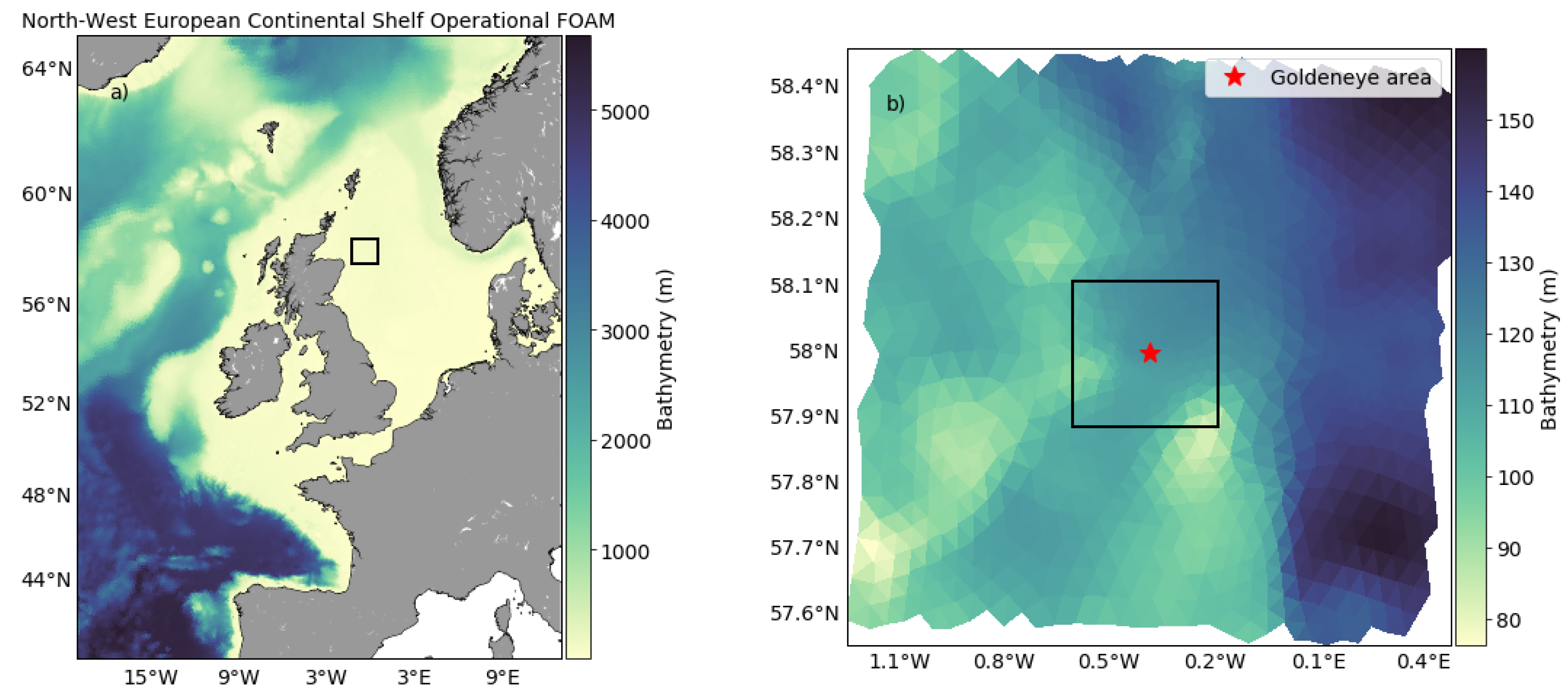
3. Case Study—Goldeneye CCS Site

3.1. Data

The data used in this study has been produced with FVCOM coupled with a biochemical tracer model, ERSEM via the framework for aquatic biogeochemical models coupler [48]. This framework provides spatio-temporal time series (4D) for both carbon chemistry and biological processes, and can model the natural variability of CO${}_2$ transportation in the oceans. Furthermore, it is possible to produce artificial leaks on the seafloor that blend with the natural variation, to produce realistic simulations of CO${}_2$-leaks. Cazenave et al. [56] produced a data set to present an approach to design marine monitoring networks for CO${}_2$ storage, where they used a weighted greedy algorithm to identify, based on a limited number of sample stations, spots that give best possible coverage. Here we adopt the CO${}_2$ concentration data from Cazenave et al. simulations, after some preprocessing steps, as input for the probabilistic deep-learning framework. The data from Cazenave et al. consist of four different simulations, one without any leakage, i.e., only the natural variability, and three with leak at the center of the domain with three different release rates. These different simulations are referred to as scenarios, and are labeled 0T (or no-leak), 30T, 300T and 3000T. The labeling are based on the amount of tons CO${}_2$ that is released per day in each simulation. We refer the reader to the paper [56] for more details about the simulations, setup and the different scenarios in general. Figure 1 shows the depth at the Goldeneye area where the leak simulations was conducted.

3.1.1. Description of Data Set

The simulation output consists of a 4D dataset, three spatial dimensions; latitude, longitude and depth as well as a fourth time dimension. There are in total 1736 nodes and 24 layer that make up an irregular triangulation in the latitude-longitude dimension and the resolution is refined near the leak. In the depth dimension sigma layers are used that is the resolution varies with the bathymetry. There are 1736 × 24 = 41,664 (nodes and layers) time series for each simulation and the time series has 1345 time steps. The time between each time step is 15 min, which means the simulations last for approximately 14 days. The data has been split in two with respect to time, where the layer closest to the seafloor in the second half of the data set is used for testing and the first half of the time series is used for training and validation. The 4 simulations we received resulted in a total of 166,656 time series of which $70\%$ of the data in the first split have been used for training and $30\%$ validation. After labeling the data (see Section 3.1.2), the training and validation data consisted of $24.2\%$ and $75.8\%$ time series labeled as leak and no-leak respectively. The test data consisted of $36.2\%$ time series labeled as leak and $69.8\%$ time series as no-leak. See

Table 1. Overview of the train, validation and test data.

	Leak	No-Leak	# Time Series	Start/End
Training Data	75.8%	24.2%	116,659	Start
Validation Data	75.8%	24.2%	49,997	Start
Test Data	69.8%	36.2%	6944	End

.

3.1.2. Preprocessing of Data

There have been five main steps of preprocessing before the data is fed to the model: Removal of time steps, splitting of the time series into two, labeling of data, time lag differencing and standardization of the data. First of all we remove the first 245 time steps of the original data due to a spin-up period of the hydrodynamic simulations, such that the data to be used further have a time dimension of 1100. Secondly, we split the data in two, using the first 550 time steps as training and validation and the last 550 time steps as test data. This is done so the test data becomes less correlated with the training and validation data sets. One of the simulations are without any leakage, and by subtracting the relevant values from the simulation with leak from the one without gives the true footprint of the leakage. Based on the true footprint a threshold can be chosen to label time series as either leak or no-leak. The recommended uncertainty measure from [57] on dissolved inorganic carbon is 1 $\mathsf{\mu }$mol/kg and corresponds to approximately $1.0236$ m mol/m${}^3$ (which is the output of the hydrodynamic simulations) with a density of seawater of $1023.6$ kg/m${}^3$. The density will change with depth and location. Here we use a threshold of 0.01 mmol/m${}^3$ such that if the true footprint at some point has been above this value the corresponding time series will be labeled as a leak. The two last steps of the preprocessing is to apply the difference transform and standardize the data. Applying a difference transform can help stabilize the mean of the time series by removing changes in the level of a time series and so eliminating and reducing trend and seasonality. Instead of assessing the time series itself changes in the signal is analyzed (an approximation of the derivative). Blackford et al. studied changes in the pH to determine if a leak was present in [39]. It makes sense to apply the difference transform in an anomaly detection perspective, where abnormal changes and patterns in the time series can be a good indicator if a leakage is present or not. Standardization of the data should improve the conditioning of the optimization problem, and speed up the training process.

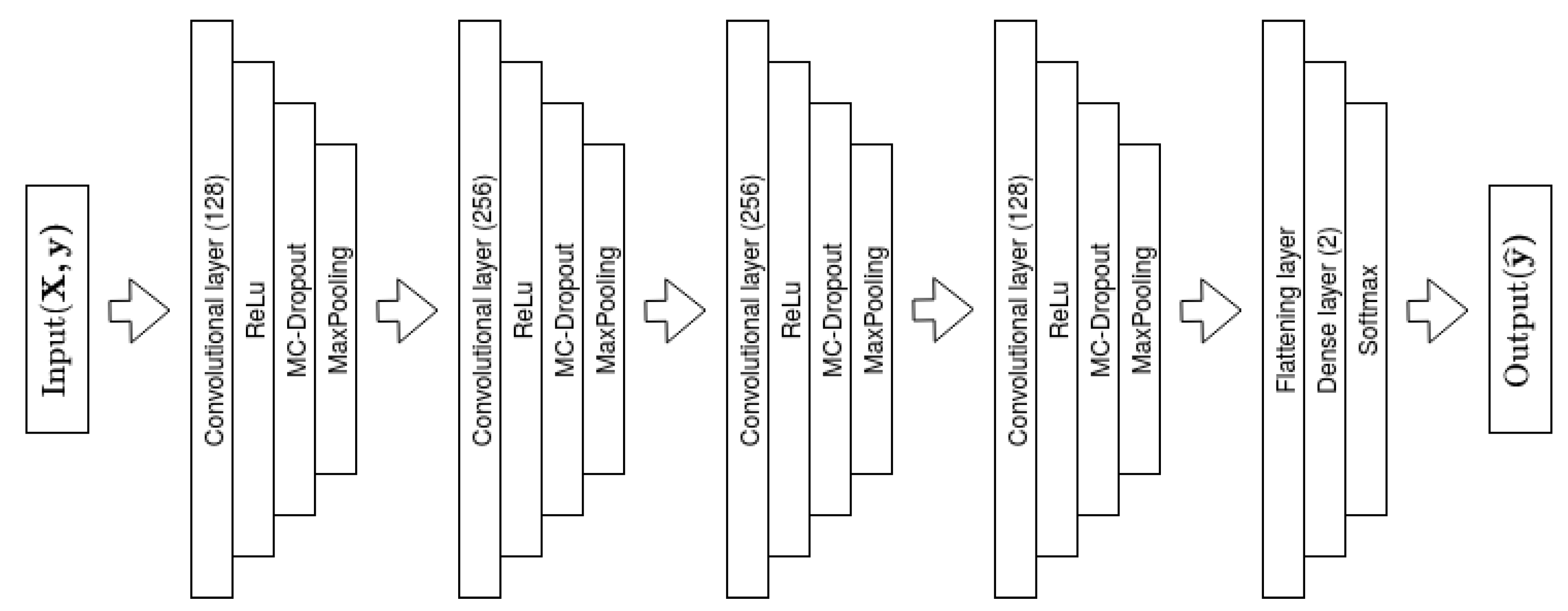
3.2. Model for TSC: Bayesian Convolutional Neural Networks

We use a traditional 1D Convolutional Neural Network model to classify time series. The model has 4 convolutional layers with ReLu activation functions [58], each followed by a MC dropout and MaxPooling layer, where MaxPooling is a down-sampling technique in convolutional neural networks. The first and last convolutional layers have 128 filters, while the middle layers both have filter size of 256. The kernel size of the convolutional layers is $\{7,5,3,2\}$ from first to last and we apply a stride of 1. We use the same dropout rate of $50\%$ for all MC dropout layers and all MaxPooling layers have a pool size of 2. The dropout rate of $50\%$ gives the largest variance over the model weights. Interpreting dropout as an ensemble of networks, a dropout rate of $50\%$ produces most possible combinations, and thus the largest variability over weights and posterior predictive distribution. According to Baldi et al. [59], the $50\%$ rate results in the strongest regularization effect, but has the disadvantage of potentially worse convergence than other dropout rates. There may exist dropout rates that gives better accuracy. However, to maximize the variance of the predictive posterior distribution, $50\%$ rate is favorable. The last part of the model is a flattening layer followed by a dense layer with two nodes and SoftMax activation function, resulting in two SoftMax probabilities, one for each class. An illustration of the model is presented in Figure 2.

Mathematically we can express the model in terms of the weights, bias and activation functions

$$\widehat{\mathbf{y}}={\sigma }_S({\sigma }_R\left({\sigma }_R\left({\sigma }_R\left({\sigma }_R(\mathbf{x}{\widehat{\mathbf{W}}}_1+\mathbf{b}){\widehat{\mathbf{W}}}_2\right){\widehat{\mathbf{W}}}_3\right){\widehat{\mathbf{W}}}_4\right){\mathbf{W}}_5.$$

Here the subscript S and R refer to a SoftMax and ReLu activation functions, respectively. The $\widehat{{\mathbf{W}}_l}$ notation, indicates that nodes are dropped out with a Bernoulli distribution, and that there are in total four layers $l=\{1,2,3,4,5\}$. It is only the first four layers that include MC dropout regularization. The model has 435842 trainable parameters and for optimization of the we use the well-known ADAM [60] algorithm. The goal is to find the parameters $\varphi =\{{\mathbf{W}}_1,{\mathbf{W}}_2,{\mathbf{W}}_3,{\mathbf{W}}_4,{\mathbf{W}}_5,\mathbf{b}\}$ such that the ${\widehat{\mathcal{L}}}_{dropout}\left(\varphi \right)$ is minimized; see Equation (3). A early stopping regime is also introduced to avoid overfitting and the validation loss is monitored and the optimization stopped after 50 epochs if no improvement is observed. We used a batch size of 256 and monitored both the accuracy and the loss. An illustration of the convergence of the training and validation of the model is showed in Figure 3.

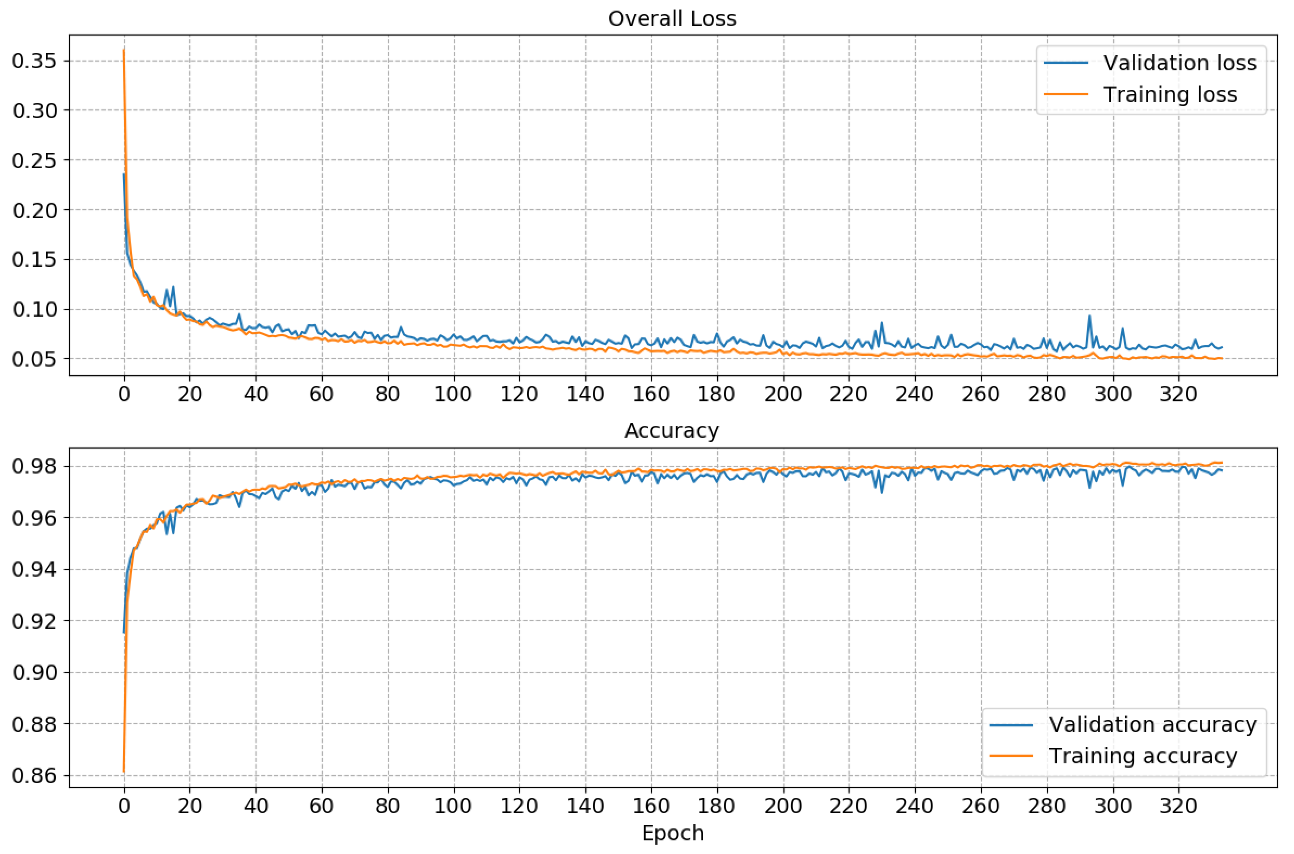
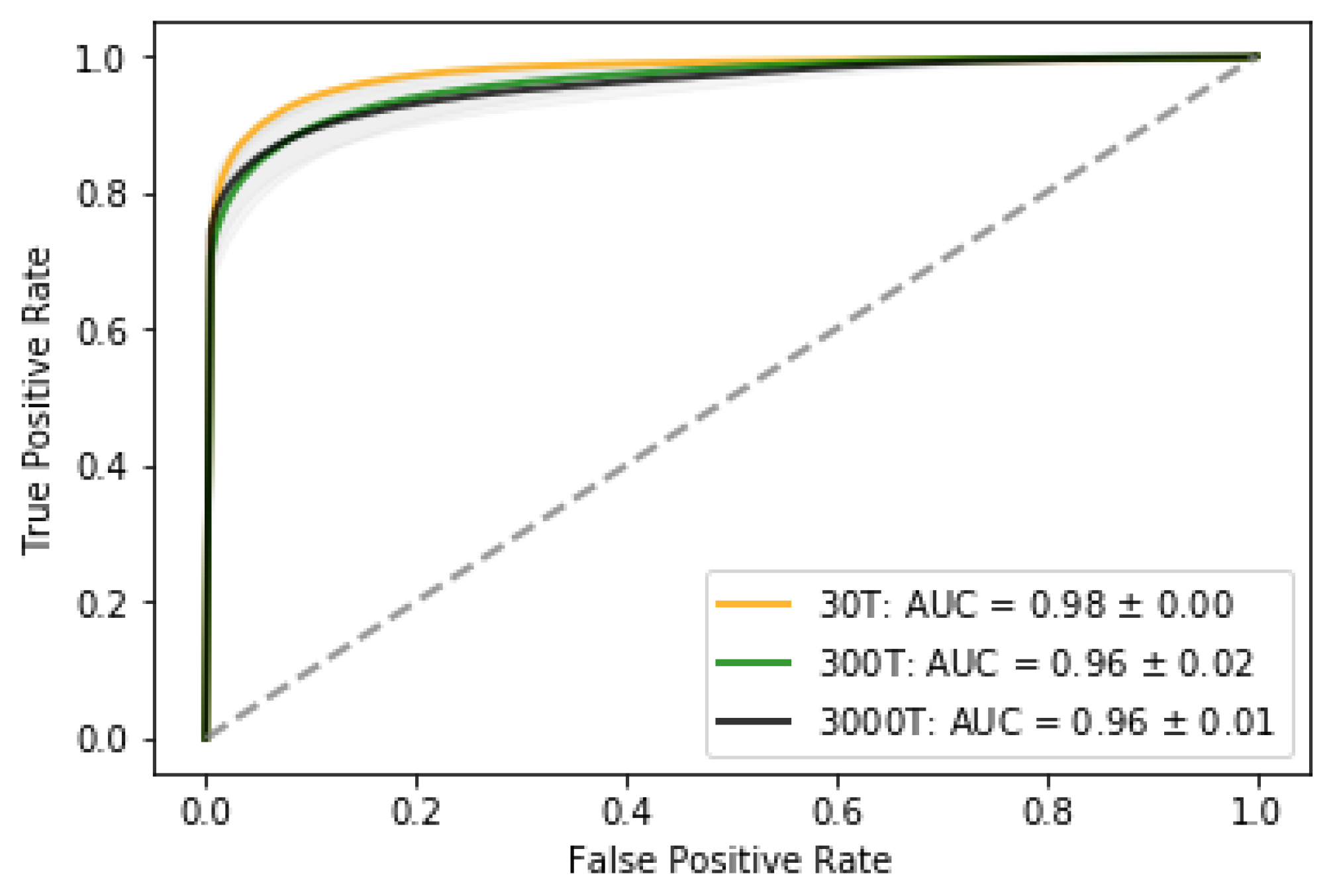
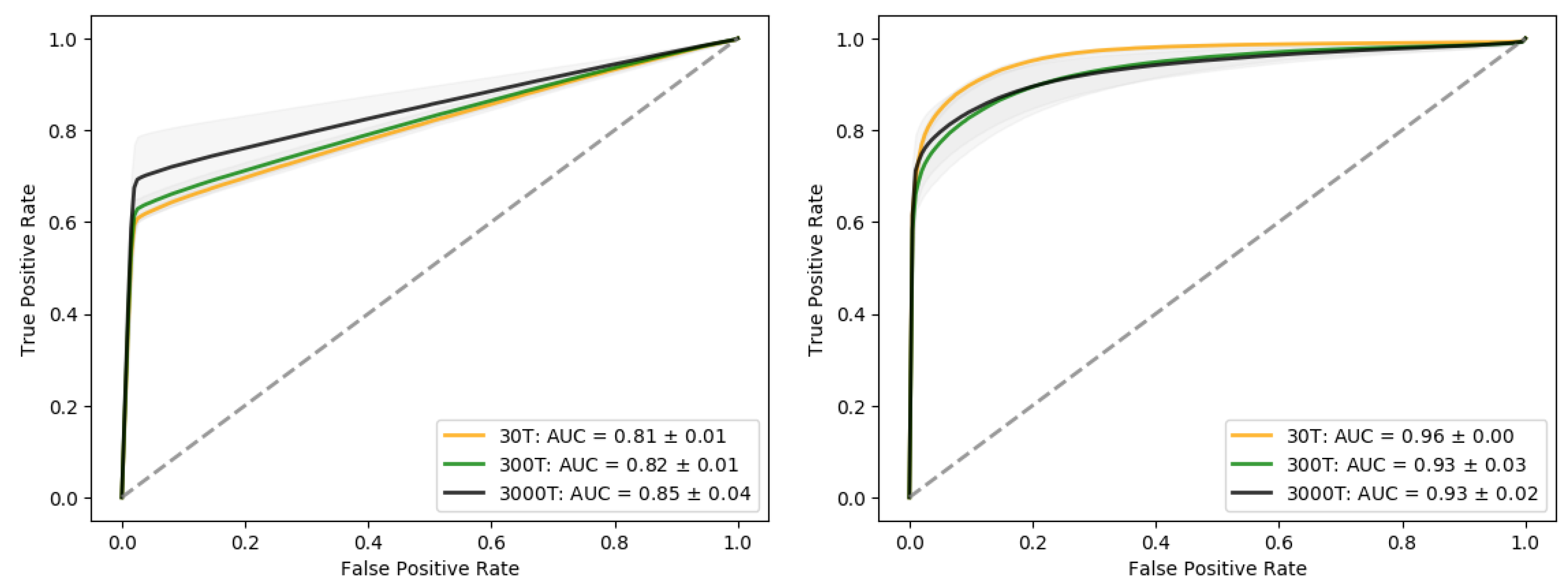
3.3. Performance of the Classifier

Figure 4 shows the proportion of true positive vs. true negatives and the Area Under the Curve (AUC). Higher the AUC indicates that the model is better at distinguishing between leak and no leak. Given the costs associated with true positives/negatives and false negatives/positives these characteristics will be useful for designing monitoring program and decision-making in mobilizing the leak confirmation phase.

In Figure 5, we show two histograms of the prediction probability and standard deviation split by the different scenarios. If we concentrate on the edges on the prediction probability histogram we see that the majority of the time series is classified as no-leak or leak and falls within the first and last bins, indicating good classification capabilities. The 0T scenario is not represented on the right-hand side of the histogram which is in line with our expectations as the classifier should not predict leaks when there is none. Smaller leaks have also fewer time series that are classified as leaks, which is intuitively since leaks with larger flux have a more distinct footprint that can be transported further. Assessing the histogram of the standard deviation, it is observed that smaller leaks scenarios have more spread than larger ones. A larger leak has a stronger signal and thus is easier to classify.

In Figure 6 the rolling mean and standard deviations with respect to the different scenarios is plotted against the distance from the leak location. We have used a quite high window size of 50 to catch and visualize trends in the data. 30T, 300T and 3000T scenario have a high confident in its prediction to about $0.1,0.3$ and 1–2 km, respectively. After this the classifier becomes less confident that there is a leakage present. For the 0T scenario a corresponding decrease in confident is observed, until it reaches its peak around 4 km. The most uncertain area of the 0T scenario coincides with the most uncertain area of the leak scenarios. That is the region from approximately 1 to 10 km from the leakage.

Calculating the area under the graph for each of the scenarios in Figure 6 gives us information on the detectability of each scenario and what scenario that are associated with highest uncertainty. The 0T scenario have the lowest area under the graph for both the prediction probability and the standard deviation, meaning that on average this is the scenario associated with highest predictive power but also the lowest uncertainty (For the 0T scenario the target is a prediction probability of 0 and not 1 as for the other scenarios). With increasing flux we observe increased area under the graph, indicating that larger flux is related to detection further away from the source. It is also observed a decrease in area under the graph for the standard deviation, indicating that smaller leaks are associated with higher degree of uncertainty. We refer to both

Table 2. Approximation of area under the graph for the different scenarios for both prediction and standard deviation.

Scenario	Prediction Probability	Standard Deviation
0T	90.15	115.48
30T	624.25	183.54
300T	633.58	161.82
3000T	773.77	153.94

and Figure 6.

Figure 7 shows a 2D histogram of the entire test data set, i.e., all scenarios combined, where the prediction probability is plotted against the standard deviation. Due to high density around 0 and 1 the color that represent the density has log-scale. As in showed in Figure 5 it is observed that the majority of the time series are close to 0 and 1, i.e., the model classifies with high confident either leak or no-leak. There are however time series that are difficult to distinguish, which have both high standard deviation and indefinite prediction probability. Making a decision under such conditions is difficult. The framework for how to decide what action to take under some cost is discussed and presented in Section 3.7.

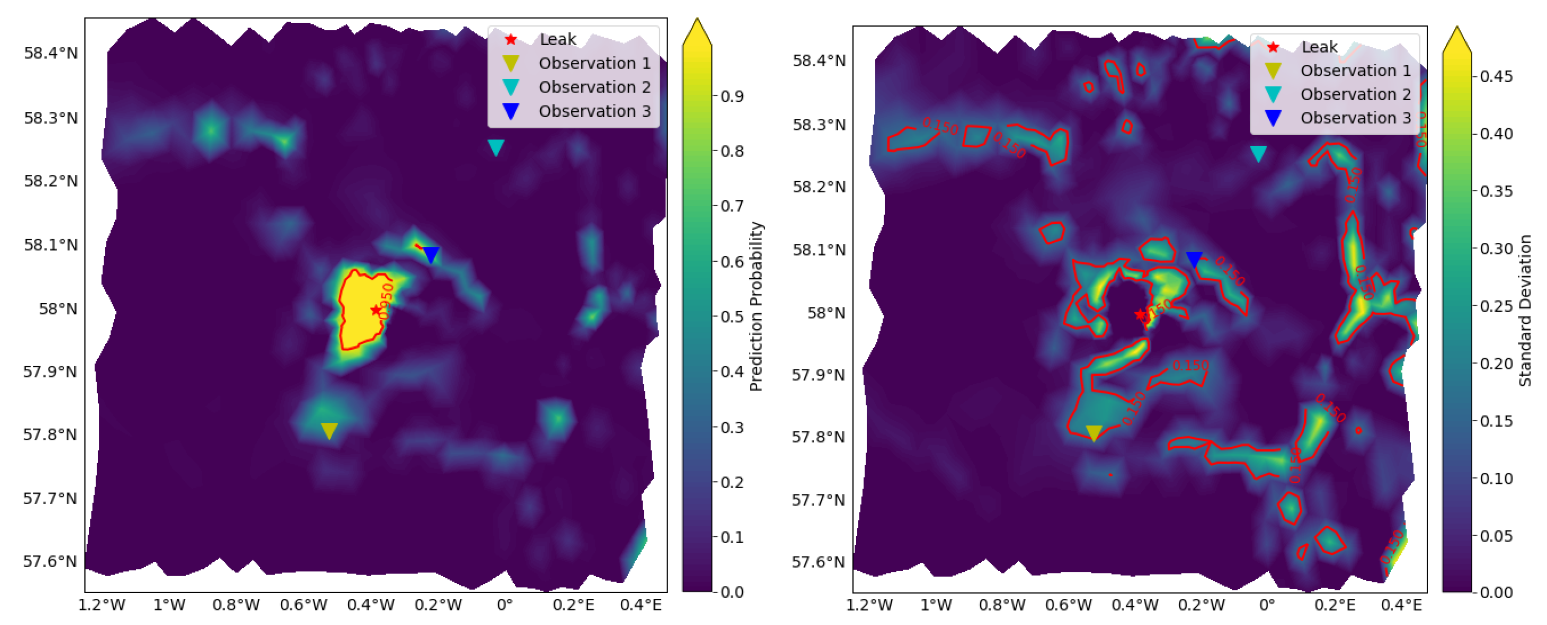
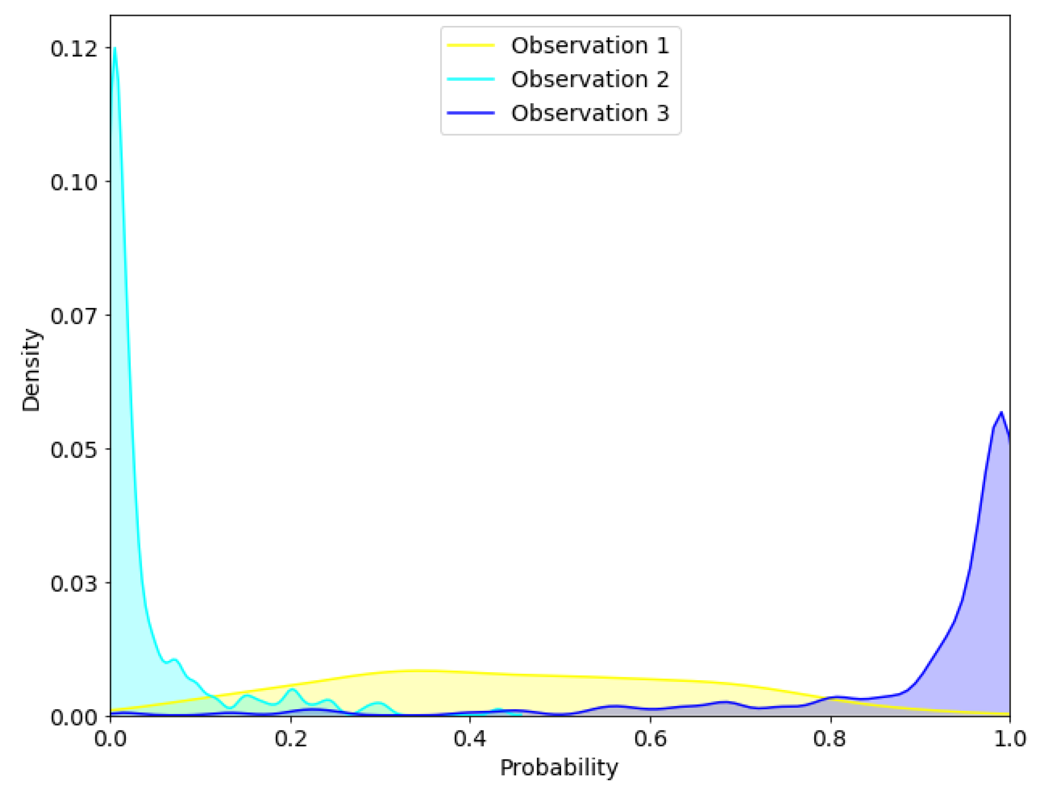
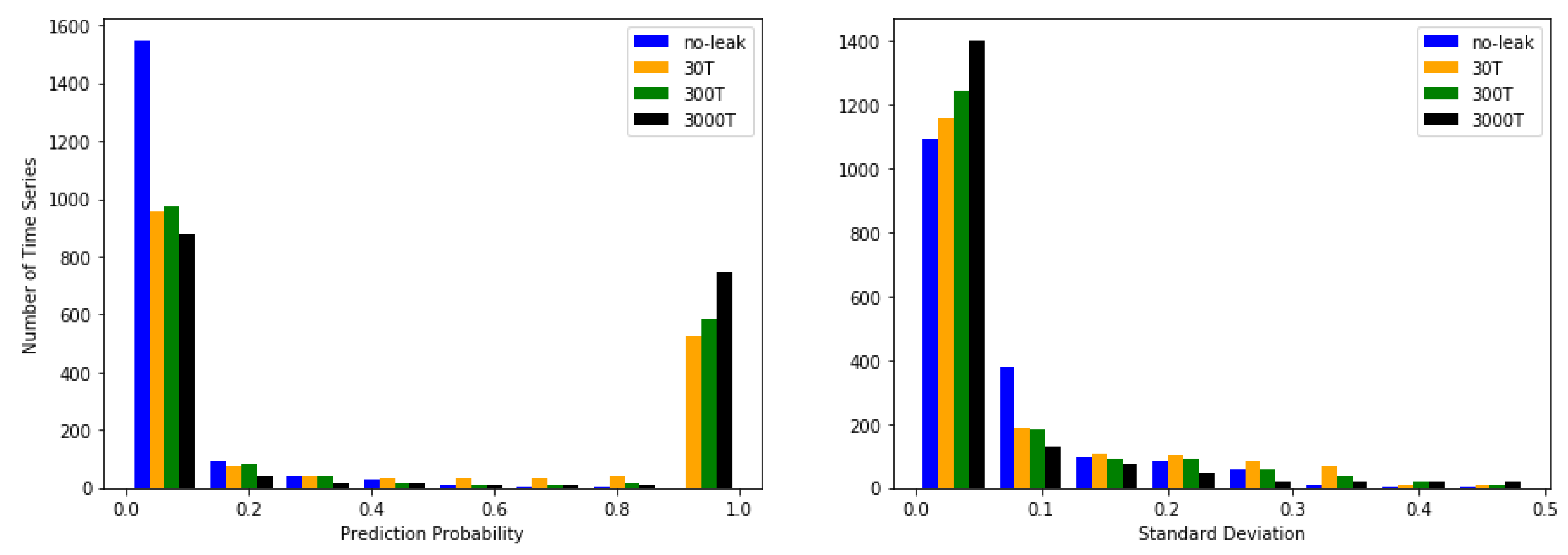
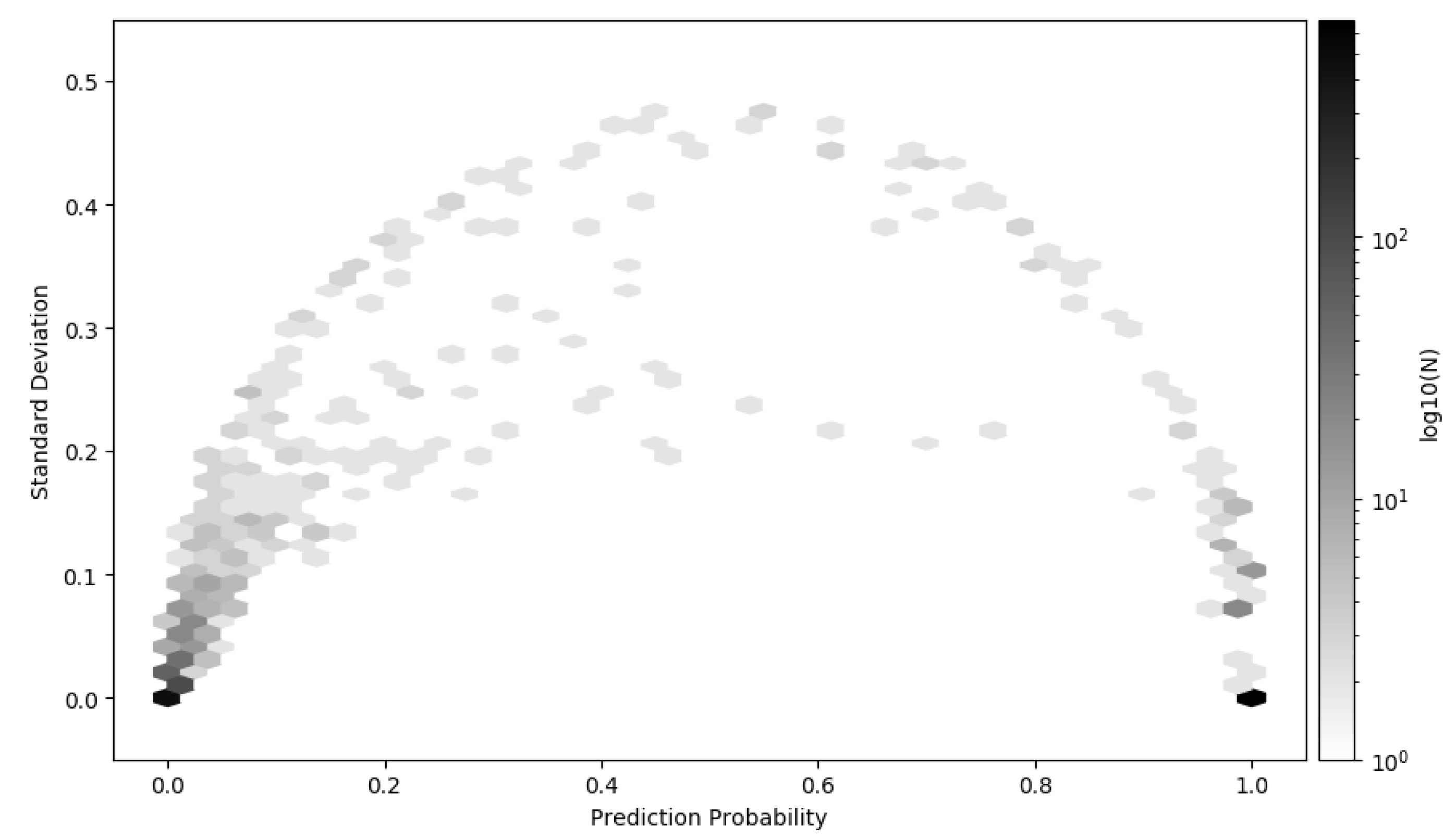
3.4. Approximated Predictive Mean and Uncertainty

In Figure 8 we see that the accuracy around the leakage is high. We also observe areas with quite high uncertainty. Due to the nature of the deep-learning methods, it is difficult to get insight in why some regions are more uncertain than other. We can only expect the classifier to detect leaks if traces of the leak have reached that particular point. There may be several reasons why we see this behavior: The training and validation data may be too different from the test data. Time series data from the two classes may be too alike, making it very difficult to distinguish the classes, or the natural variability and a leak behave in some regions similar. The classifier will in these cases have a hard task, and in some cases misclassify or be uncertain about the prediction.

Figure 9 shows kernel density estimates (KDE) of the 200 forward MC realizations for the three different locations in Figure 8. The yellow KDE is from the area south, in a region with high uncertainty. The distribution is almost uniform, making it very difficult to say if the time series arise from a leak situation. The blue KDE predicts that the time series arise from a leakage situation, with quite high confidence. This is reasonable, as the measurement is quite close to the leak locations. The cyan KDE shows relatively little spread, with a clear indication that this arise from a no-leak situation. Because of the distance from the leak location, this is reasonable, as traces from the leak might not reached this region of the area. One of the key concepts here has been to show how to model uncertainty in time series with modern deep-learning techniques. We therefore did not put a tremendous effort into optimization of hyper-parameters of the BCNN to improve the accuracy and decrease the uncertainty.

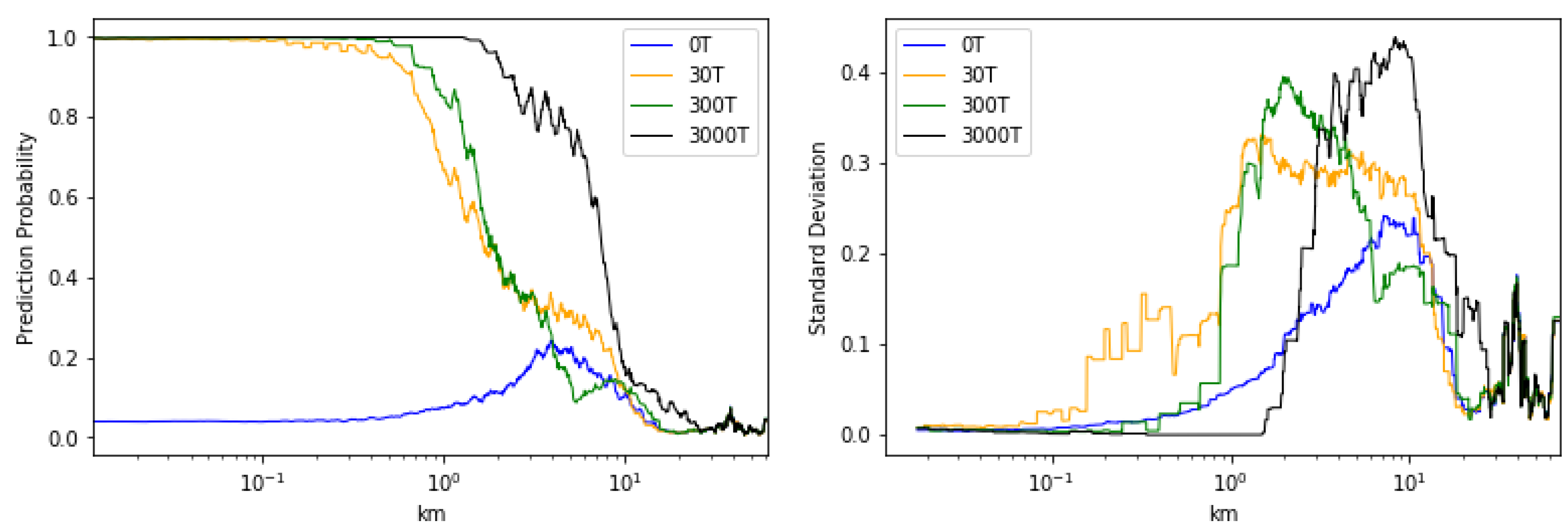
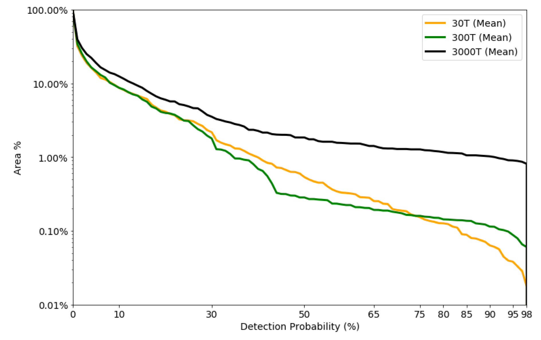
3.5. Detectable Area vs. Detection Probability

In Figure 10, we have plotted the area covered against the detection probability. First we observe that the detected area is greater with larger leakages. Secondly, the 30T and 300T scenario have small difference in percentage of area detected up to approximately $80\%$ detection probability. Thirdly, if we demand high prediction probability the different leak scenarios can detect an area around 1–10%, 0.1–1% and 0.1–0.01% for the 3000T, 300T, and 30T leak scenario, respectively. This gives us insight on the size of the footprint we can detect and thus some insight in how to optimize sensor layout. Simulated leaks have been used to predict footprints subsequently being used to optimize sensor layout [61,62,63,64,65]. They used a threshold that was based on the Cseep method [66] that is dependent on measurements of different biochemical tracers. We argue that using deep-learning methods and BCNN can lower this threshold, increasing the detectable footprints and thus the decreasing the number of sensors needed to monitor a specific area.

3.6. Sensitivity Analysis

We have validated the model in the bottom layer only, because this is where the sensors can be placed. We have additionally made two sanity checks on the generalization properties of the approach. The first is related to how sensitive the method is if we train only on the simulations with 0T, 30T and 3000T and test this new trained model on the test data set. The second address the sensitivity if we add some stochastic Gaussian noise to the test data.

3.6.1. Reducing the Training Data Set

The model was optimized similar to as described in Section 3.2, the only difference is that the 300T simulation scenario is removed from the training data set. The ROC for the case where the 300T scenario is removed from the training data set is presented in the right panel of Figure 11, with associated AUC values. We observe that the AUC value is relatively high in the case with 300T, despite no training on leaks with such size. The overall AUC is high in all cases, but with an increased uncertainty compared to AUC values in Figure 4. In general the AUC values are relatively large compared to training with all simulated scenarios. This suggest that the model generalizes well.

3.6.2. Adding Gaussian Noise the Test Data Set

We briefly assess the classifiers sensitivity by adding Gaussian Noise, $\mathcal{N}(0,\sigma ),$ to the test data set, before we predict by using the same trained model as above. The noise was added to the pre-processed time series of the test data set. We tested two cases, where we chose $\sigma =0.01$ and $\sigma =0.1$.

The general observation for a relatively low level of noise ($\sigma =0.01$), is that time series with true label no-leak had a higher uncertainty related to its prediction and the predicted value of it being labeled as leak increased. That is the AUC has dropped from values near 1, see Figure 4, to values around $0.8$, see Figure 11. The prediction of true leaks were improved, however at the cost of more false positives. With a noise level of $0.1$, the majority of the time series were classified as leaks. This tells us that this classifier is sensitive to small and rapid changes in the data, for data where the true label is no-leak, which can lead us to two potential conclusions. Either rapid and relatively small changes is a potential indicator of a leakage, or the classification is just comprised due to the additional noise. There are studies using rapid changes as indicators of leaks, as described by Blackford et al. in [39]. This also highlights major drawbacks of deep-learning methods, i.e., it is difficult to interpret the model and to explain classification criteria. It is worth mentioning that if the noise also were added to the training data, the classifier might cater for this and be more robust against such changes.

3.7. Making Decisions Based on BCNN Output with Varying Cost

In Section 2.7 we presented Algorithm 1 that can assist in taking difficult decisions during environmental monitoring. The reminder of this Section exemplifies the use of Algorithm 1, given a specific cost function. We have created $T=200$ realizations as an approximation of the two posterior distributions $P_t\left(c_1\right|{\mathbf{x}}^{*})$ and $P_t\left(c_2\right|{\mathbf{x}}^{*})$. Since we use binary classification, we have that $P_t\left(c_2\right|{\mathbf{x}}^{*})=1-P_t\left(c_1\right|{\mathbf{x}}^{*})$. The 200 realization can be viewed as distinct expert opinions of what class the time series belongs. By applying the two summary function Equations (5) and (6) to the posterior predictive distribution we get the following decision rule in the binary classification setting, that is, we decide action ${\alpha }_1$ if

$$({\lambda }_{21}-{\lambda }_{11})P\left(c_1\right|{\mathbf{x}}^{*})>({\lambda }_{12}-{\lambda }_{22})P\left(c_2\right|{\mathbf{x}}^{*}).$$

Since it is difficult to estimate the real cost associated with confirming a leakage, we use a simple cost function and vary some parameters to determine the impact of the cost function on the optimal decision. The cost associated with confirming a no-leak situation is the baseline cost, i.e., we assign a value of 1 for this purpose. This cost can be interpreted as the operational cost with sending a cruise or initiate a unmanned operation to check for a leakage. We assume that the cost with confirming a leakage is dependent on the operational cost. Furthermore, the cost of not confirming a leakage is $\kappa$ times more expensive than the operational cost. The parameter $\gamma$ is the factor that describes the cost of not confirming a leakage compared to the cost of confirming a leakage. The cost associated with not confirming if there is no leakage is assumed to be 0. Based on these assumptions we can set up a decision rule dependent on the summary function over the posterior distribution; confirm a leak if

$$(\gamma -1)\kappa >\frac{P\left(c_1\right|{\mathbf{x}}^{*})}{P\left(c_2\right|{\mathbf{x}}^{*})}.$$

(7)

Table 3. Overview of the cost functions applied in this example. The cost function can be interpreted as having no cost to doing the correct decision. Confirming a no-leak has some operational cost, e.g., a ship must mobilize and search/confirm that there is no leakage. Confirm a leakage has a cost of $\kappa$ times the operational cost. The cost of not confirming a true leakage is gamma times the cost of confirming a leakage. We assume there is no cost with not looking for a leak when there is no leakage.

	Leak	No-Leak
Confirm (${\alpha }_1$)	${\lambda }_{11}=\kappa$	${\lambda }_{12}=1$
Not Confirm (${\alpha }_2$)	${\lambda }_{21}=\gamma {\lambda }_{11}$	${\lambda }_{22}=$ 0

shows the cost function in terms of true and false positives and true and false negatives.

In Figure 12 we show the percentage of the total area to be monitored for $\kappa \in \{10,100,1000\}$ and $1\le \gamma \le 100.$

This cost function shows the trade-off between confirming a leak and not confirming a leak. By using the MAP, the predictive distribution becomes more distinct on which class it belongs. We see this in Figure 12, where the percentage area needed to be monitored under the same cost function is significantly lower.

4. Discussion

We have presented a three-step algorithm that combines BCNNs with Bayesian decision theory, for support in environmental monitoring. In the first step a BCNN is optimize on labeled simulated data. In the next step, the BCNN is used to generate a posterior predictive distribution of class labels. In the final step, the optimal monitoring strategy is calculated based on the posterior predictive distribution and given operational costs.

Our case study indicates that MC dropout and BCNN are effective tools for detecting CO${}_2$ seeps in marine waters. The overall predictive power is large, as seen through the ROC curve in Figure 4. While the majority of the time series are either classified as leak or no-leak with little uncertainty, a small proportion will be inconclusive; see Figure 5. As expected, the classification uncertainties increase with the distance to the leak source location. This distance depends on the seep flux rates and can be modeled from the outcome of the BCNN; see Figure 6.

Demanding high detection probability reduces the detectable area of a monitoring location, i.e., you will need to measure closer to a leak in order to achieve the desired accuracy; see Figure 10. This motivates the use of optimal decision strategies, that is finding appropriate action that should be initiated based on the prediction, its uncertainty, and costs associated with taking wrong and right decisions. We gave an example of an optimal strategy choice in a binary classification setting in Section 3.7 for different costs, showcasing the algorithm.

There is extensive literature, including several deep-learning approaches, on monitoring and forecasting of air quality time series. For example Biancofiore et al. [35] used a recursive and feed forward neural network and Freeman et al. [36] a RNN to forecast and monitor air quality from time series data. In context of oceanography monitoring, Bezdek et al. [67] used hyper-ellipsoidal models for detecting anomalies in a wireless sensor network and validated their approach on data from Great Barrier Reef. None of these approaches take uncertainty into account. Ahmad [68] recently published a literature review of machine-learning applications in oceanography.

As CO${}_2$ is naturally present in the ocean and is highly variable, it is difficult to attribute measured CO${}_2$ to an unplanned release. Blackford et al. [39] developed pH anomaly criterion for determination of marine CO${}_2$ leaks. This criterion is however location dependent and cannot be generalized. In contrast to Blackford et al., our method automatically extracts features and characteristics that could be hidden within the natural variability, potentially increasing the detection probability. Due to the costly survey in case of confirmation of leakages, it will be of importance with information about the model’s uncertainty, our approach provides that.

The most important strength of our approach is that it is principled and consistently uses a probabilistic Bayesian framework for effective decision-making in the context of environmental monitoring. A potential weakness of our case study is that we did not systematically optimize hyper-parameters, which could potentially improve the results. Examples are increasing or decrease the number of CNN layers, changing activation functions, loss functions, optimization procedures, and size of filters, strides and kernel size of the convolutional layers. With respect to loss function and activation function, we have chosen the standard techniques used in the machine-learning community today and have not addressed these norms. With respect to size of filters, strides and kernel size of the convolutional layers, we have only performed a small trial and error search of the possible hyper-parameters. Looking into the model’s weights shows that quite a large part of the network is active, suggesting that the model structure and size is relatively well-balanced. We have not found it feasible to use a lot of time to tune the model further, as we have achieved good results with the current hyper-parameter configuration.

Another more serious limitation is the fact that the BCNN is optimized with data based on a limited number of simulations for a limited time period. This biases the BCNN model towards the simulated conditions. The model can still be used in a general scenario, but its predictive power will decrease. That is why more simulations with different forcing, leak locations and fluxes are necessary to generate a predictive model that is more robust.

To test how well our BCNN model generalizes, we have carried out some sensitivity analyses in Section 3.6. The general observation was that adding noise to the test data increased uncertainty and decreased predictive accuracy. With low level of noise the prediction deteriorates, mainly because no-leak time series is miss-classified as leaks, false positives. However, it is still able to distinguish the two classes with relatively good success. Corruption of deep-learning models is a well know problem, even with small alterations in the input data. This problem might have been solved by training the model on noisy data.

A second sensitivity analysis showed that removal of the 300T data set reduced the overall predictive power in all cases; however, the method was still able with high confident and accuracy to predict the 300T test data set. This indicates at least good generalization properties to different leakage fluxes, and potentially to different leakage locations.

In this study, univariate time series was used; however, if more information were available in terms of different sensors, measuring different geochemical markers, this framework could be extended to a multi-variate TSC setting. Another extension could be to increase the number of classes and treat them as a multi-label classification tasks, with the purpose to classify time series as be either of the following classes; 0T, 30T, 300T or 3000T.

Another question we would like to study is how well our model generalizes to different locations. One of the key concepts of CNNs is the ability to extract important features from the data. Here the concept capability to capture key characteristics of time series that contain a leak signal or not. In this sense, the model should generalize well to other locations. Testing this hypothesis would be an important step towards wide-spread use of our method.

However, in our view, the most interesting extension would be to extend the framework to a transfer learning setting. The concept of transfer learning is to use a pre-trained model and fix the weights of the first few layers and re-train with an entirely new data set. Transfer learning has been used with success in computer vision and other tasks, and the key benefit is that the need for data is reduced drastically. Translation of this concept to binary TSC, where the pre-trained model would be trained on simulation data, should be investigated closer.

References

1. Halpern, B.S.; Longo, C.; Hardy, D.; McLeod, K.L.; Samhouri, J.F.; Katona, S.K.; Kleisner, K.; Lester, S.E.; O’Leary, J.; Ranelletti, M.; et al. An index to assess the health and benefits of the global ocean. Nature 2012, 488, 615–620. [Google Scholar] [CrossRef] [PubMed] [Green Version]
2. Domínguez-Tejo, E.; Metternicht, G.; Johnston, E.; Hedge, L. Marine Spatial Planning advancing the Ecosystem-Based Approach to coastal zone management: A review. Mar. Policy 2016, 72, 115–130. [Google Scholar] [CrossRef]
3. Ali, A.; Thiem, Ø.; Berntsen, J. Numerical modelling of organic waste dispersion from fjord located fish farms. Ocean Dyn. 2011, 61, 977–989. [Google Scholar] [CrossRef] [Green Version]
4. Hylland, K.; Burgeot, T.; Martínez-Gómez, C.; Lang, T.; Robinson, C.D.; Svavarsson, J.; Thain, J.E.; Vethaak, A.D.; Gubbins, M.J. How can we quantify impacts of contaminants in marine ecosystems? The ICON project. Mar. Environ. Res. 2017, 24, 2–10. [Google Scholar] [CrossRef] [PubMed] [Green Version]
5. First, P.J. Global Warming of 1.5 C an IPCC Special Report on the Impacts of Global Warming of 1.5 C above Pre-Industrial Levels and Related Global Greenhouse Gas Emission Pathways, in the Context of Strengthening the Global Response to the Threat of Climate Change. Sustain. Dev. Efforts Eradicate Poverty 2019, 1, 1–22. [Google Scholar]
6. Agency, I.E. Global Energy & CO2 Status Report; Technical Report; IEA: Paris, France, 2018. [Google Scholar]
7. Bauer, S.; Beyer, C.; Dethlefsen, F.; Dietrich, P.; Duttmann, R.; Ebert, M.; Feeser, V.; Görke, U.; Köber, R.; Kolditz, O.; et al. Impacts of the use of the geological subsurface for energy storage: An investigation concept. Environ. Earth Sci. 2013, 70, 3935–3943. [Google Scholar] [CrossRef]
8. Blackford, J.; Bull, J.M.; Cevatoglu, M.; Connelly, D.; Hauton, C.; James, R.H.; Lichtschlag, A.; Stahl, H.; Widdicombe, S.; Wright, I.C. Marine baseline and monitoring strategies for carbon dioxide capture and storage (CCS). Int. J. Greenh. Gas Control 2015, 38, 221–229. [Google Scholar] [CrossRef] [Green Version]
9. Jones, D.; Beaubien, S.; Blackford, J.; Foekema, E.; Lions, J.; Vittor, C.D.; West, J.; Widdicombe, S.; Hauton, C.; Queirós, A. Developments since 2005 in understanding potential environmental impacts of {CO2} leakage from geological storage. Int. J. Greenh. Gas Control 2015, 40, 350–377. [Google Scholar] [CrossRef] [Green Version]
10. Yang, Q.; Wu, X. 10 challenging problems in data mining research. Int. J. Inf. Technol. Decis. Mak. 2006, 5, 597–604. [Google Scholar] [CrossRef] [Green Version]
11. Esling, P.; Agon, C. Time-series data mining. ACM Comput. Surv. (CSUR) 2012, 45, 12. [Google Scholar] [CrossRef] [Green Version]
12. Bagnall, A.; Lines, J.; Bostrom, A.; Large, J.; Keogh, E. The great time series classification bake off: A review and experimental evaluation of recent algorithmic advances. Data Min. Knowl. Discov. 2017, 31, 606–660. [Google Scholar] [CrossRef] [PubMed] [Green Version]
13. Berndt, D.J.; Clifford, J. Using Dynamic Time Warping to Find Patterns in Time Series; KDD Workshop: Seattle, WA, USA, 1994; Volume 10, pp. 359–370. [Google Scholar]
14. Ratanamahatana, C.A.; Keogh, E. Three myths about dynamic time warping data mining. In Proceedings of the 2005 SIAM International Conference on Data Mining, SIAM, Newport Beach, CA, USA, 21–23 April 2005; pp. 506–510. [Google Scholar]
15. Bagnall, A.; Janacek, G. A run length transformation for discriminating between auto regressive time series. J. Classif. 2014, 31, 154–178. [Google Scholar] [CrossRef] [Green Version]
16. Smyth, P. Clustering Sequences with Hidden Markov Models. Available online: http://papers.nips.cc/paper/1217-clustering-sequences-with-hidden-markov-models.pdf (accessed on 1 June 2020).
17. Williams, C.K.; Barber, D. Bayesian classification with Gaussian processes. IEEE Trans. Pattern Anal. Mach. Intell. 1998, 20, 1342–1351. [Google Scholar] [CrossRef] [Green Version]
18. James, G.M.; Hastie, T.J. Functional linear discriminant analysis for irregularly sampled curves. J. R. Stat. Soc. Ser. B 2001, 63, 533–550. [Google Scholar] [CrossRef]
19. Hall, P.; Poskitt, D.S.; Presnell, B. A functional data—Analytic approach to signal discrimination. Technometrics 2001, 43, 1–9. [Google Scholar] [CrossRef]
20. Bagnall, A.; Lines, J.; Hills, J.; Bostrom, A. Time-series classification with COTE: The collective of transformation-based ensembles. IEEE Trans. Knowl. Data Eng. 2015, 27, 2522–2535. [Google Scholar] [CrossRef]
21. Lines, J.; Taylor, S.; Bagnall, A. Time Series Classification with HIVE-COTE: The Hierarchical Vote Collective of Transformation-Based Ensembles. ACM Trans. Knowl. Discov. Data 2018, 12. [Google Scholar] [CrossRef] [Green Version]
22. Fawaz, H.I.; Forestier, G.; Weber, J.; Idoumghar, L.; Muller, P.A. Deep learning for time series classification: A review. Data Min. Knowl. Discov. 2019, 33, 1–47. [Google Scholar]
23. Zheng, Y.; Liu, Q.; Chen, E.; Ge, Y.; Zhao, J.L. Time series classification using multi-channels deep convolutional neural networks. In Proceedings of the International Conference on Web-Age Information Management, Macau, China, 16–18 June 2014; pp. 298–310. [Google Scholar]
24. Wang, Z.; Yan, W.; Oates, T. Time series classification from scratch with deep neural networks: A strong baseline. In Proceedings of the 2017 International Joint Conference on Neural Networks (IJCNN), Anchorage, AK, USA, 14–19 May 2017; pp. 1578–1585. [Google Scholar]
25. Hüsken, M.; Stagge, P. Recurrent neural networks for time series classification. Neurocomputing 2003, 50, 223–235. [Google Scholar] [CrossRef]
26. MacKay, D.J.C. A Practical Bayesian Framework for Backpropagation Networks. Neural Comput. 1992, 4, 448–472. [Google Scholar] [CrossRef]
27. Alendal, G.; Blackford, J.; Chen, B.; Avlesen, H.; Omar, A. Using Bayes Theorem to Quantify and Reduce Uncertainties when Monitoring Varying Marine Environments for Indications of a Leak. Energy Procedia 2017, 114, 3607–3612. [Google Scholar] [CrossRef]
28. Gal, Y.; Ghahramani, Z. Dropout as a Bayesian approximation: Representing model uncertainty in deep learning. In Proceedings of the International Conference on Machine Learning, New York, NY, USA, 19–24 June 2016; pp. 1050–1059. [Google Scholar]
29. Blundell, C.; Cornebise, J.; Kavukcuoglu, K.; Wierstra, D. Weight uncertainty in neural networks. arXiv 2015, arXiv:1505.05424. [Google Scholar]
30. Shridhar, K.; Laumann, F.; Liwicki, M. A comprehensive guide to bayesian convolutional neural network with variational inference. arXiv 2019, arXiv:1901.02731. [Google Scholar]
31. Leibig, C.; Allken, V.; Ayhan, M.S.; Berens, P.; Wahl, S. Leveraging uncertainty information from deep neural networks for disease detection. Sci. Rep. 2017, 7, 17816. [Google Scholar] [CrossRef] [PubMed] [Green Version]
32. Abideen, Z.U.; Ghafoor, M.; Munir, K.; Saqib, M.; Ullah, A.; Zia, T.; Tariq, S.A.; Ahmed, G.; Zahra, A. Uncertainty Assisted Robust Tuberculosis Identification With Bayesian Convolutional Neural Networks. IEEE Access 2020, 8, 22812–22825. [Google Scholar] [CrossRef]
33. Kendall, A.; Cipolla, R. Modelling uncertainty in deep learning for camera relocalization. In Proceedings of the 2016 IEEE International Conference on Robotics and Automation (ICRA), Stockholm, Sweden, 16–21 May 2016; pp. 4762–4769. [Google Scholar]
34. Malde, K.; Handegard, N.O.; Eikvil, L.; Salberg, A.B. Machine intelligence and the data-driven future of marine science. ICES J. Mar. Sci. 2019. [Google Scholar] [CrossRef]
35. Biancofiore, F.; Busilacchio, M.; Verdecchia, M.; Tomassetti, B.; Aruffo, E.; Bianco, S.; Di Tommaso, S.; Colangeli, C.; Rosatelli, G.; Di Carlo, P. Recursive neural network model for analysis and forecast of PM10 and PM2.5. Atmos. Pollut. Res. 2017, 8, 652–659. [Google Scholar] [CrossRef]
36. Freeman, B.S.; Taylor, G.; Gharabaghi, B.; Thé, J. Forecasting air quality time series using deep learning. J. Air Waste Manag. Assoc. 2018, 68, 866–886. [Google Scholar] [CrossRef] [PubMed]
37. Kiiveri, H.; Caccetta, P.; Campbell, N.; Evans, F.; Furby, S.; Wallace, J. Environmental Monitoring Using a Time Series of Satellite Images and Other Spatial Data Sets. In Nonlinear Estimation and Classification; Denison, D.D., Hansen, M.H., Holmes, C.C., Mallick, B., Yu, B., Eds.; Springer: New York, NY, USA, 2003; pp. 49–62. [Google Scholar] [CrossRef]
38. Banskota, A.; Kayastha, N.; Falkowski, M.J.; Wulder, M.A.; Froese, R.E.; White, J.C. Forest Monitoring Using Landsat Time Series Data: A Review. Can. J. Remote Sens. 2014, 40, 362–384. [Google Scholar] [CrossRef]
39. Blackford, J.; Artioli, Y.; Clark, J.; de Mora, L. Monitoring of offshore geological carbon storage integrity: Implications of natural variability in the marine system and the assessment of anomaly detection criteria. Int. J. Greenh. Gas Control 2017, 64, 99–112. [Google Scholar] [CrossRef]
40. Siddorn, J.R.; Allen, J.I.; Blackford, J.C.; Gilbert, F.J.; Holt, J.T.; Holt, M.W.; Osborne, J.P.; Proctor, R.; Mills, D.K. Modelling the hydrodynamics and ecosystem of the North-West European continental shelf for operational oceanography. J. Mar. Syst. 2007, 65, 417–429. [Google Scholar] [CrossRef]
41. Alendal, G.; Drange, H. Two-phase, near-field modeling of purposefully released CO2 in the ocean. J. Geophys. Res. Ocean. 2001, 106, 1085–1096. [Google Scholar] [CrossRef]
42. Dewar, M.; Sellami, N.; Chen, B. Dynamics of rising CO2 bubble plumes in the QICS field experiment. Int. J. Greenh. Gas Control 2014. [Google Scholar] [CrossRef] [Green Version]
43. Ali, A.; Frøysa, H.G.; Avlesen, H.; Alendal, G. Simulating spatial and temporal varying CO2 signals from sources at the seafloor to help designing risk-based monitoring programs. J. Geophys. Res. Ocean. 2016, 121, 745–757. [Google Scholar] [CrossRef] [Green Version]
44. Blackford, J.; Alendal, G.; Avlesen, H.; Brereton, A.; Cazenave, P.W.; Chen, B.; Dewar, M.; Holt, J.; Phelps, J. Impact and detectability of hypothetical CCS offshore seep scenarios as an aid to storage assurance and risk assessment. Int. J. Greenh. Gas Control 2020, 95, 102949. [Google Scholar] [CrossRef]
45. Vielstädte, L.; Karstens, J.; Haeckel, M.; Schmidt, M.; Linke, P.; Reimann, S.; Liebetrau, V.; McGinnis, D.F.; Wallmann, K. Quantification of methane emissions at abandoned gas wells in the Central North Sea. Mar. Pet. Geol. 2015, 68, 848–860. [Google Scholar] [CrossRef]
46. Pan, S.J.; Yang, Q. A survey on transfer learning. IEEE Trans. Knowl. Data Eng. 2009, 22, 1345–1359. [Google Scholar] [CrossRef]
47. Chen, C. An Unstructured-Grid, Finite-Volume Community Ocean Model: FVCOM User Manual; Sea Grant College Program, Massachusetts Institute of Technology: Cambridge, MA, USA, 2012. [Google Scholar]
48. Butenschön, M.; Clark, J.; Aldridge, J.N.; Allen, J.I.; Artioli, Y.; Blackford, J.; Bruggeman, J.; Cazenave, P.; Ciavatta, S.; Kay, S.; et al. ERSEM 15.06: A generic model for marine biogeochemistry and the ecosystem dynamics of the lower trophic levels. Geosci. Model Dev. 2016, 9, 1293–1339. [Google Scholar]
49. Hähnel, P.; Mareček, J.; Monteil, J.; O’Donncha, F. Using deep learning to extend the range of air pollution monitoring and forecasting. J. Comput. Phys. 2020, 408, 109278. [Google Scholar] [CrossRef] [Green Version]
50. Ruthotto, L.; Haber, E. Deep neural networks motivated by partial differential equations. J. Math. Imaging Vis. 2019, 62, 1–13. [Google Scholar] [CrossRef] [Green Version]
51. Gal, Y. Uncertainty in Deep Learning. Ph.D. Thesis, University of Cambridge, Cambridge, UK, 2016. [Google Scholar]
52. Gal, Y.; Ghahramani, Z. Bayesian convolutional neural networks with Bernoulli approximate variational inference. arXiv 2015, arXiv:1506.02158. [Google Scholar]
53. Srivastava, N.; Hinton, G.; Krizhevsky, A.; Sutskever, I.; Salakhutdinov, R. Dropout: A simple way to prevent neural networks from overfitting. J. Mach. Learn. Res. 2014, 15, 1929–1958. [Google Scholar]
54. Tibshirani, R.J.; Efron, B. An introduction to the bootstrap. Monogr. Stat. Appl. Probab. 1993, 57, 1–436. [Google Scholar]
55. Berger, J.O. Statistical Decision Theory and Bayesian Analysis; Springer Science & Business Media: Berlin/Heidelberg, Germany, 2013. [Google Scholar]
56. Cazenave, P.; Blackford, J.; Artioli, Y. Regional Modelling to Inform the Design of Sub-Sea CO2 Storage Monitoring Networks. In Proceedings of the 14th Greenhouse Gas Control Technologies Conference Melbourne, Melbourne, Australia, 21–26 October 2018; pp. 21–26. [Google Scholar]
57. Riebesell, U.; Fabry, V.J.; Hansson, L.; Gattuso, J.P. Guide to Best Practices for Ocean Acidification Research and Data Reporting; Office for Official Publications of the European Communities: Brussels, Belgium, 2011.
58. Nair, V.; Hinton, G.E. Rectified linear units improve restricted boltzmann machines. In Proceedings of the 27th International Conference on Machine Learning (ICML-10), Haifa, Israel, 21–24 June 2010; pp. 807–814. [Google Scholar]
59. Baldi, P.; Sadowski, P. The dropout learning algorithm. Artif. Intell. 2014, 210, 78–122. [Google Scholar] [CrossRef] [Green Version]
60. Kingma, D.P.; Ba, J. Adam: A method for stochastic optimization. arXiv 2014, arXiv:1412.6980. [Google Scholar]
61. Hvidevold, H.K.; Alendal, G.; Johannessen, T.; Ali, A.; Mannseth, T.; Avlesen, H. Layout of CCS monitoring infrastructure with highest probability of detecting a footprint of a CO2 leak in a varying marine environment. Int. J. Greenh. Gas Control 2015, 37, 274–279. [Google Scholar] [CrossRef] [Green Version]
62. Greenwood, J.; Craig, P.; Hardman-Mountford, N. Coastal monitoring strategy for geochemical detection of fugitive CO2 seeps from the seabed. Int. J. Greenh. Gas Control 2015, 39, 74–78. [Google Scholar] [CrossRef]
63. Hvidevold, H.K.; Alendal, G.; Johannessen, T.; Ali, A. Survey strategies to quantify and optimize detecting probability of a CO2 seep in a varying marine environment. Environ. Model. Softw. 2016, 83, 303–309. [Google Scholar] [CrossRef] [Green Version]
64. Alendal, G. Cost efficient environmental survey paths for detecting continuous tracer discharges. J. Geophys. Res. Ocean. 2017, 122, 5458–5467. [Google Scholar] [CrossRef] [Green Version]
65. Oleynik, A.; García-Ibáñez, M.I.; Blaser, N.; Omar, A.; Alendal, G. Optimal sensors placement for detecting CO2 discharges from unknown locations on the seafloor. Int. J. Greenh. Gas Control 2020, 95, 102951. [Google Scholar] [CrossRef]
66. Botnen, H.; Omar, A.; Thorseth, I.; Johannessen, T.; Alendal, G. The effect of submarine CO2 vents on seawater: Implications for detection of subsea Carbon sequestration leakage. Limnol. Oceanogr. 2015, 60, 402–410. [Google Scholar] [CrossRef]
67. Bezdek, J.C.; Rajasegarar, S.; Moshtaghi, M.; Leckie, C.; Palaniswami, M.; Havens, T.C. Anomaly detection in environmental monitoring networks [application notes]. IEEE Comput. Intell. Mag. 2011, 6, 52–58. [Google Scholar] [CrossRef]
68. Ahmad, H. Machine learning applications in oceanography. Aquat. Res. 2019, 2, 161–169. [Google Scholar] [CrossRef]
Figure 1. (a) FVCOM domain used in which resolution varies from 15 km at the open boundaries to 0.5 km at the release site. The black box indicates the extents of the grid shown in (b). (b) The nested domain with resolution from 0.5 km at the boundary to 3 m at the release site (red star). The black box in (b) indicates the extent of the Goldeneye complex [56].
Algorithms 13 00145 g001
Figure 2. Illustration of the Bayesian Convolutional Neural Network Model used.
Algorithms 13 00145 g002
Figure 3. Convergence of the BCNN. In total it ran for 334 epochs, approximately two hours of train/validation time with a NVIDIA Titan V GPU.
Algorithms 13 00145 g003
Figure 4. ROC-curves for the three leak scenarios. The 0T scenario is not included since it in all cases will be classified as no-leak, i.e., there are no false positives.
Algorithms 13 00145 g004
Figure 5. (Left Panel) Prediction probability for each scenario plotted as a histogram. (Right Panel) Standard deviation for each scenario plotted as a histogram. The central observation is that most of the time series is classified as either leak = 0 or No - leak = 1 . Minor leaks have a smaller proportion of the time series that are classified as leaks than larger ones and smaller leaks are associated with a higher degree of uncertainty than the larger ones.
Algorithms 13 00145 g005
Figure 6. (Right panel) A moving mean of the prediction probability vs. the distance from the leakage. (Left panel) A moving standard deviation vs. the distance from the leakage. For the moving statistics, all points are evenly weighted.
Algorithms 13 00145 g006
Figure 7. 2D histogram of the mean prediction and standard deviation of all the time series in the test data set. The majority of the time series are predicted near 0 or 1 with low standard deviation. The color pallet have log-scale to visualize the time series that are classified with high standard deviation and low distinction in the prediction probability.
Algorithms 13 00145 g007
Figure 8. Prediction from the BCNN on the 3000T test data. (Left panel) The plot shows the predictive mean leak probability of the 1736 nodes with 200 forward MC realization on each instance. The red line shows where the predictive mean leak probability is above a value of 0.95. (Right panel) The plot shows the uncertainty in the prediction. Red line shows where the standard deviation is above 0.15 indicating areas where the prediction is uncertain. See Figure 9 for more details about the uncertainty in observation locations 1, 2, and 3.
Algorithms 13 00145 g008
Figure 9. Kernel density estimation (KDE) of the three observations in Figure 8. We have used the seaborn visualization library, i.e., Gaussian kernel with Scott method for estimation the kernel bandwidth. The KDE smoothens the empirical distribution, thus exceeding the estimate beyond the possible range of [ 0 , 1 ] . We thus limit the plot to be within the bounds, which means that this KDE does not summarize to 1.
Algorithms 13 00145 g009
Figure 10. Mean detection probability plotted vs. the total area covered at specific threshold.
Algorithms 13 00145 g010
Figure 11. (Left panel) ROC curve with Gaussian noise is simulated with a standard deviation of 0.01 is added to the test data set. The drop of in accuracy is quite large, even with relatively low level of noise added to the test data. (Right Panel) ROC curve for the case where we have excluded the 300T scenario.
Algorithms 13 00145 g011
Figure 12. The figure shows the percentage of the total area to be monitored where the optimal decision would be confirming a leak. The cost function is altered by varying the parameter κ and γ in Equation (7) and Table 3. The three different lines represents varying κ , and the the x-axis shows varying γ for each scenario. Increased cost difference between the operational cost and the cost of confirming a leak, result in a higher degree of confirmation, faster. (Left Panel) The MAP of the predictive posterior distribution. (Right Panel) The expectation of the predictive posterior distribution. Using the mode instead of the expectation results in less confirmation/mobilization.
Algorithms 13 00145 g012