DS Evidence Theory-Based Energy Balanced Routing Algorithm for Network Lifetime Enhancement in WSN-Assisted IOT


State Key Laboratory of Alternate Electrical Power System with Renewable Energy Sources, North China, Electric Power University, Beijing 102206, China
*
Author to whom correspondence should be addressed.
Algorithms 2020, 13(6), 152; https://0-doi-org.brum.beds.ac.uk/10.3390/a13060152
Submission received: 25 May 2020
/
Revised: 16 June 2020
/
Accepted: 22 June 2020
/
Published: 24 June 2020
(This article belongs to the Section Combinatorial Optimization, Graph, and Network Algorithms)
Abstract
:Wireless sensor networks (WSNs) can provide data acquisition for long-term environment monitoring, which are important parts of Internet of Things (IoT). In the WSN-assisted IoT, energy efficient routing algorithms are required to maintain a long network lifetime. In this paper, a DS evidence theory-based energy balanced routing algorithm for network lifetime enhancement (EBRA-NLE) in WSN-assisted IOT is proposed. From the perspective of energy balance and minimization of routing path energy consumption, three attribute indexes are established to evaluate the forward neighboring nodes. Then a route selection method based on DS evidence theory is developed to comprehensively evaluate the nodes and select the optimal next hop. In order to avoid missing the ideal solution because of the excessive difference between the index values, the sine function is used to adjust this difference. The simulation results show that the proposed EBRA-NLE has certain advantages in prolonging network lifetime and balancing energy between nodes.
1. Introduction
WSN-assisted IOT is used for data collection in the environment and detect the certain events of significance in the physical world. It can bring great convenience to people’s life [1,2,3,4], such as environmental monitoring, military tracking, and health observations. Sensor nodes send the sensed information to the base station (BS) by single hop or multi-hops. Therefore, the energy consumption and location deployment of the nodes can affect the network lifetime. The sensor nodes are generally powered by battery, which can only maintain a limited lifetime because of the limited energy, and the cost of replacing the battery is relatively expensive and hard to achieve. Numerous researches have shown that the energy consumption of nodes in WSNs is mainly in data transmission during routing [5]. Therefore, how to design energy balanced and efficient routing algorithms to prolong network lifetime is the key to the development of WSN-assisted IOT.
There are a lot of existing routing protocols to extend the network lifetime, which are mainly divided into three aspects: (1) minimize the path energy consumption. Minimizing the path energy consumption is to save the energy of the entire network by adopting the shortest routing path or reducing path relay hops [6]. (2) Balance the energy between nodes. This method tries to consume the energy of the nodes in the network as evenly as possible, thereby delaying the death of the first node and extending the network lifetime. (3) Transmission power control. To reduce energy consumption of data transmission, the methods of transmission power control measure and model RSS (received signal strength) to obtain optimal data transmission power, which is used to decrease channel interference among sensor nodes [7,8,9]. However, once the path failure happens, the related nodes need to re-establish the network topology [10].
Based on the above observations, in order to balance and efficiently utilize energy to extend the network lifetime, we propose an energy-balanced routing algorithm for network lifetime enhancement (EBRA-NLE) based on DS evidence theory [11]. DS evidence theory can fuse multiple attributes according to DS fusion rules and make the optimal choice, so it is applied to our routing selection for WSNs. Our main contributions are summarized as follows:
- In WSN, many previous researches on DS evidence theory mainly focus on data fusion to enhance the reliability and security of information acquisition, but the application of indexes fusion in sensor nodes as a routing decision-making method is very few. In this paper, we adopt DS fusion rules to fuse three attribute indexes that affecting energy balance and energy efficiency of each node.
- First, the node’s forward neighboring nodes are taken as the evaluation object, and three indexes are established as evaluation objects from the perspective of energy balance, minimization of path energy consumption, and buffer proportion. It should be noted that, in order to reflect the importance of each index according to the difference in attributes between nodes, a sine function is adopted to map the belief function corresponding to each index. Then DS fusion rule is utilized to comprehensively evaluate the indexes of each node to obtain the optimal path selection.
- Simulation results show that the proposed EBRA-NLE has certain advantages in prolonging network lifetime and balancing energy between nodes. In addition, the network lifetime obtained by EBRA-NLE is improved about 313% and 72% more than that of MCRP and DS-EERA algorithm respectively.
The rest of the paper is organized as follows: Section 2 reviews the related research works. The system model is introduced in Section 3. The EBRA-NLE algorithm is presented in detail in Section 4. The relevant simulation results are analyzed and discussed in Section 5. Finally, the conclusion is summarized in Section 6.
2. Related Works
For these energy saving algorithms of minimizing the energy consumption [12,13,14], some routing strategies establish the shortest path from the source node to the destination, so that the path energy consumption in data transmission is the lowest. Among them, a ladder diffusion algorithm based on ACO (ant colony optimization) is proposed to solve the problem of energy consumption in routing [12], which mainly employed ACO mechanism to effectively reduce path energy consumption. Although the shortest path can reduce the energy consumption of data transmission, it is easy to cause the energy imbalance between nodes because of the lack of consideration of residual energy, which leads to the death of some key nodes because of the premature depletion of energy. In addition, a routing algorithm named dynamic optimal progress routing (DOPR) uses a hybrid routing-mobility strategy to guarantee message delivery [13], it moves the intermediate nodes on the selected path to proper positions to reduce the energy consumption of nodes. Bouabdallah et al. [14] put forward SCMR routing algorithm. The SCMR adopts active reporting node selection mechanism of correlation radius, which can inhibit the data transmission of redundant nodes, thus reducing network energy consumption.
In terms of extending the network lifetime by balancing the residual energy between nodes [15,16,17,18,19,20,21], Behzadan et al. in [15] proposed a distributed ED balanced based on a theoretic heterogeneous balanced data routing (HBDR) algorithm for routing, while the inter-node interference was not be considered. Petrioli et al. [16] presented distributed GRP and localized ALBA-R for balancing traffic load of nodes that are located around connectivity holes so that the nodes do not run out of energy too fast. Mehmmood et al. [17] developed an algorithm that the nodes consume their energy balanced by both region and node level. In this protocol, the evolutionary game theory (EGT) and classical game theory (CGT) are used to balance the traffic load. Gupta and Jha proposed an improved energy balance clustering protocol based on cuckoo search [18], which adopts an objective function to evenly distribute cluster heads. Then use the cuckoo search algorithm to optimize the data transmission of the cluster head and the destination node, and finally get the purpose of energy saving to improve energy efficiency. However, these algorithms do not fully consider some important attributes of the node when selecting the next hop, such as traffic. As a result, some performance of the nodes is poor.
Therefore, some algorithms consider multiple attributes of nodes to make a comprehensive route selection [19,20,21,22]. Among them, MCRP [19] sort multiple network attribute matrices to obtain the optimal solution by TOPSIS method. Nevertheless, adopting the TOPSIS can only reflect the relative closeness of each attribute to its own ideal solution, which does not reflect the closeness to the overall ideal solution. Tang et al. [22] proposed a routing algorithm based on DS evidence theory, which uses DS evidence fusion rules to fuse the attribute indexes of nodes, and selects the best next hop according to the fusion results. Although this method can balance the energy between nodes to a certain extent, the triangular membership function is adopted in the establishment of the belief function, which may lead to too much pursuit of the ideal solution of each index so as to miss the optimal fusion result.
In addition, some methods can solve the energy hole problem by adjusting the data transmission power [7,8,9], so that the energy consumption of the whole network can be minimized and balanced. Fei et al. [7] proposed a coordinated transmission strategy, which solves the problem of network lifetime maximization and energy minimization through two different simultaneous interpreting strategies. Zeng et al. [9] presented an algorithm to avoid the “energy hole” problem with adjustable transmit power based on the distribution of network energy consumption, the lifetime of regional nodes, and the real-time data. Thus in order to prolong the network lifetime, the algorithm sends the corresponding proportion of data to the area with low energy consumption in a short communication radius. The energy hole can be alleviated by changing the transmission power to some extent, but it is difficult to determine the value of the adjustable transmission power, so it is difficult to apply it to the actual sensor networks.
3. System Model
3.1. Network Model
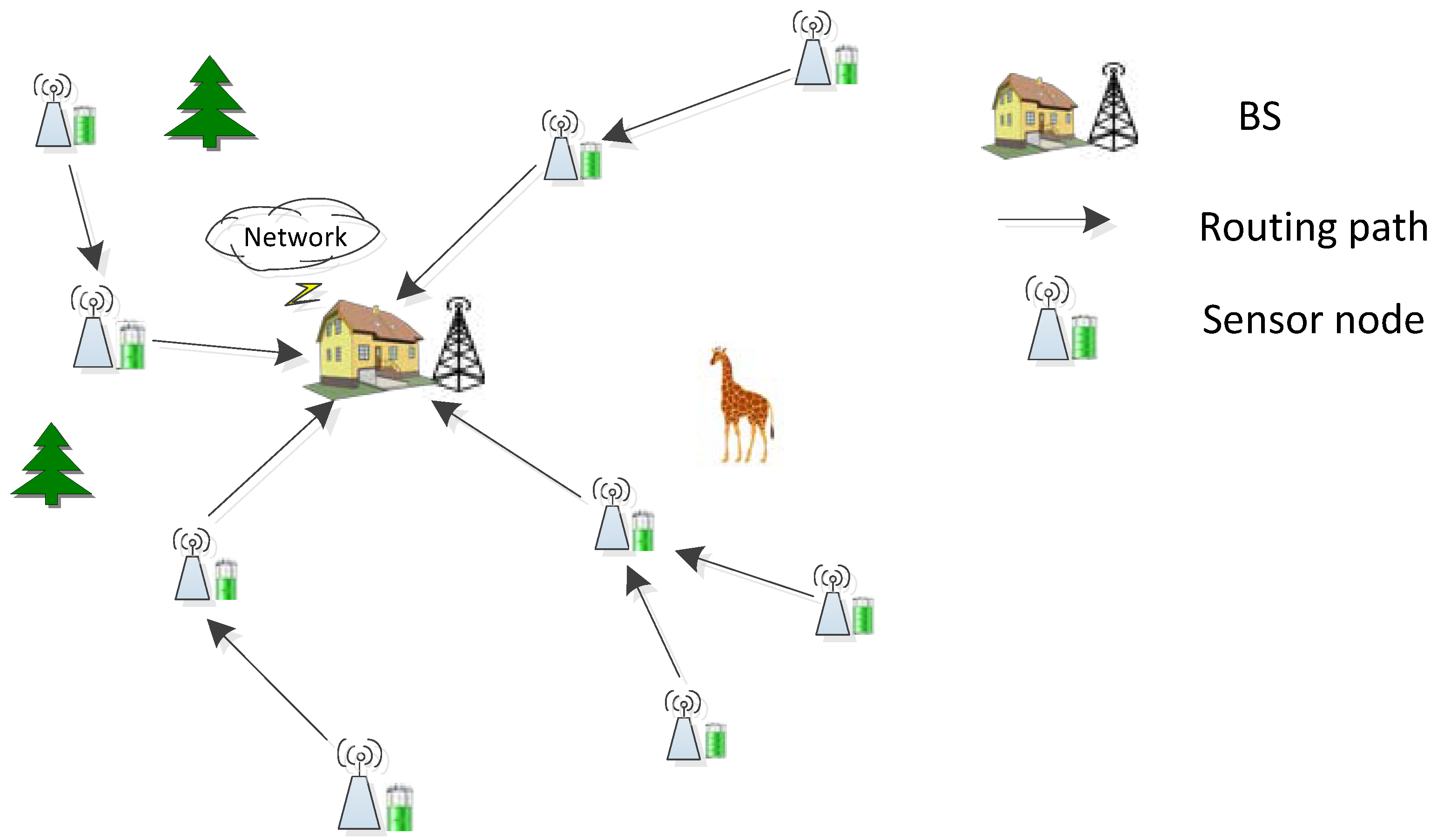
As shown in Figure 1, the sensor nodes periodically sense the data and transmit them to BS in a multi-hop manner. The network model includes a fixed BS in the center, which is used to manage nodes information. sensor nodes are randomly distributed in a square area , and the communication radius of each sensor node is set to . Meanwhile, the energy of the battery carried by each node is limited and all initial energy is . The topology of the whole network is composed of an undirected graph , where denotes all sensor nodes and is a set of directed path links between nodes. The set of forwarding neighboring nodes of node is given by:
where , denote the distance from node , node to BS respectively.
To facilitate the description of the network model, the following reasonable assumptions are presented as follows:
- (1)
- Once the network is deployed, the location of the sensor nodes will not move any more. The sensor nodes can estimate the distance to other nodes based on the received signal strength and positioning module [23]. Then the node uploads the location information to BS.
- (2)
- All sensor nodes are isomorphic, with function of routing, sending and receiving packets, and the initial status is the same.
- (3)
- Each node has a unique identifier (ID), which maintains a buffer to store information such as residual energy, next-hop ID, packet ID, sender IDs etc. The information is updated in real time as the forward neighbor changes [22].
- (4)
- It is noted that the buffer length of each node is limited, and data packets are processed in first-in first-out (FIFO) mode.
- (5)
- The time when the first node dies due to energy exhaustion is defined as network lifetime.
3.2. Energy Consumption Model
In this paper, we used a simple energy model as adopted in [22,24]. The required energy for transmitting bits data over distance is as follows:
where is the consumed energy per bit by the transmitting and receiving circuit, and is the free space loss coefficient. It is noted that since the communication range between the receiver and the sender is limited to the radius and [24] ( is the threshold distance), thus the free space ( power loss) channel model is employed in this model.
Meanwhile, the energy consumption for a node receiving bits data over distance is given by:
Thus, the energy consumption of node receiving and forwarding bits data is expressed as:
4. EBRA-NLE: DS Evidence Theory-Based Energy Balanced Routing Algorithm for Network Lifetime Enhancement
DS evidence theory was proposed by Dempster Shafer in 1970s [11], which can fuse multiple information and its fusion results are in line with people’s thinking habits. Therefore, DS evidence theory is widely used in artificial intelligence, detection, and diagnosis etc., [25]. DS evidence theory establishes a one-to-one correspondence between propositions and sets, which can transform the uncertainty of propositions into the uncertainty of sets. In this paper, we apply DS evidence theory to routing selection in WSNs. First of all, we consider the residual energy of nodes, the shortest data transmission path and the buffer proportion, so as to establish “energy balance factor,” “relay coefficient,” and “buffer idleness” as the evidences of DS fusion rules. Then DS fusion rules are applied to fuse the three indexes of corresponding belief function, thus the results of comprehensive evaluation are obtained. It should be noted that the belief function is obtained by sinusoidal mapping of membership function, so as to reflect the importance of each index in the fusion process and make the optimal routing objectively.
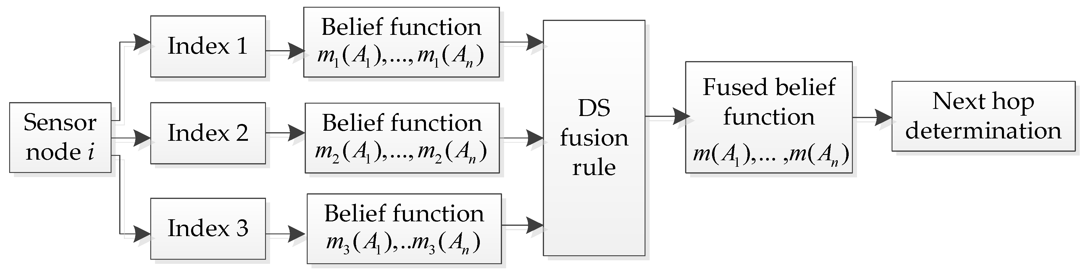
DS evidence theory is an effective method to fuse subjective uncertainty information, and its fusion decision process [26] is shown in Figure 2. Where is the number of forward neighboring nodes of node , that is . is the belief allocation of forward neighbors under different index . is the fused belief allocation of propositions of node . When calculating the probability allocation of each neighbor, it is necessary to establish attribute indexes of evaluation nodes, which will be described in the next section.
4.1. The Establishment of Attribute Indexes
4.1.1. Energy Balance Factor
Since the main energy consumption of sensor nodes is used for data transmission, the key to prolong the network lifetime is to balance the energy consumption of each source node and its next hop. From the perspective of the source node , when its residual energy is small, the energy consumption of single hop transmission is expected to be as small as possible. When the energy of node is large, it is hoped that node can transmit a longer distance, that is, the value of is as large as possible. Therefore, considering the residual energy of the node and the energy consumption of data transmission, the energy balance factor is defined as follows:
where denotes the energy consumption of data transmission from node to node , represents the energy consumption of data transmission at the longest transmission distance .
4.1.2. Relay Coefficient
During data transmission, the closer the forward neighboring node is to the shortest path from the node to the BS, the more energy can be saved in the routing path. Meanwhile, the more residual energy of the node , the more data can be forwarded to it. Thus the relay coefficient is defined as follows:
4.1.3. Buffer Idleness
Because the data transmission in WSNs has the characteristics of “many to one”, it may lead to numerous traffic data converging to some key nodes at the same time. It may run out of energy prematurely because of the overload and reduce the network lifetime. Thus these nodes discard data because of limited buffer, which will affect the reliability of data transmission. Therefore, the buffer idleness is established to measure the ability of nodes to receive data, which is expressed as follows:
where is the current traffic data of node , is the traffic flowing into the node , is the traffic flowing out of the node , and is the maximum buffer length of each node.
4.2. Acquisition of Belief Function
4.2.1. Sine Mapping Based Membership Function
The acquisition of belief function is based on membership function, so this section first introduces the establishment process of the membership function. For each node , the three attribute indexes of its forward neighbor node are presented as , which correspond to the index . All three are benefit indexes, that is, the larger the index value, the more likely it is to be selected as the next hop. The three indexes value of each forward neighbor node can be calculated, and the maximum value of each index is the optimal solution under this index. That is, , and .
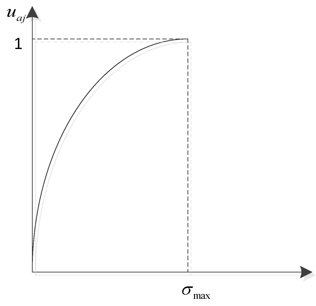
In order to avoid missing the node with the best comprehensive performance due to excessive pursuit of ideal solution, we establish the membership function based on sine function, its expression is as follows:
where .
The mapping relationship is shown in Figure 3.
4.2.2. Belief Function
The domain of evidence theory is called recognition framework , which includes a limited number of propositions and are recorded as . It corresponds to the basic event in probability theory, which is called focal element. In this paper, it corresponds to the forward neighboring nodes of each node. The propositions in are mutually exclusive. The calculation of belief function is referred to [26,27], and this paper also makes the following relevant definitions as follows:
Definition 1.
Supposeis the recognition framework. If the set function:(is the power set of) satisfy:
whereis called the belief function allocation on recognition framework. is the empty set. For,is called the belief function value of. When,is called the focal element on the allocation of belief function, that is, the reliability of a node selected as the next hop.
Definition 2.
whereis the three indexes (),is the number of forward neighbors of node. andare fixed values for the sensor network.is the weighted coefficient of the index. In this paper, . is the correlation coefficient of the attribute indexto each forward neighboring node.,,are denote the maximum correlation coefficient, the correlation allocation value and the reliability coefficient of the index.
In this paper, the membership function in fuzzy theory is used to replace the correlation coefficient [26], both of which can be used to evaluate the trust degree belonging to the next hop based on the value of the indexes of the forward neighboring nodes. Thus, the correlation coefficient of the index is . Bringing into above equations, thus , , of the forward neighboring node at the index can be obtained.
Then, the belief function of the index to the proposition corresponding to the forward neighbor node can be obtained as follows:
The function of uncertainty reliability under index is:
It can be seen from Equations (14) and (15) that weighted coefficient and the correction coefficient have certain subjectivity, which is determined by field experience and sensor characteristics.
4.3. The DS Fusion Rules of Indexes and the Routing Path Section
4.3.1. DS Fusion Rules
According to the fusion rule [26] of DS evidence theory, all forward neighboring nodes in are regarded as the propositions . First, take two indexes (that is ) as an example, let respectively correspond to the belief function assignment of two different indexes. Then, the allocation of the combined belief function is defined as follows:
where is the sum of all belief products including complete conflict hypothesis, is the belief products of non-conflict hypothesis. Conflict hypothesis means that and cannot exist at the same time, that is, they are mutually exclusive in the . The belief function value refers to the sum of all the reliability products of and , which contain the non-conflict hypothesis.
The uncertainty function values of fusion results are calculated as follows:
After the fusion of index 1 and index 2 is assigned to the belief function value of each forward neighboring node, the fusion result is taken as the belief function of the new index. Then the fusion result is obtained by the fusion with index 3 according to the Equations (16) and (18).
4.3.2. Path Selection Principle
In order to avoid the counter-intuitive and conflict results in the next hop selection, the routing decisions generally follow the following principles:
- The next hop selected should have the largest belief function value and be greater than a certain threshold.
- The difference of the belief function between the next hop and other forward neighbors is greater than a certain threshold value.
- The belief function value of the selected next hop is greater than its uncertainty function value.
The determination of the corresponding threshold is adjusted according to specific experimental scenarios. Then find with that satisfy the path selection principle and regard the node (denoted by proposition ) as the optimal next hop of node . Finally, according to this routing selection rules, all nodes in the network can get an energy balanced data transmission path from the source nodes to BS.
In order to facilitate the reader’s understanding, the routing process is formed into Algorithm 1.
| Algorithm 1. The routing path selection. |
| Input: Node |
| Output: The next hope J |
| 1. for i = 1:N do |
| 2. |
| 3. for j = 1:n do |
| 4. Calculate by Equations (5)–(7) |
| 5. end for |
| 6. , Calculate by Equation (8) |
| 7. , Calculate by Equation (8) |
| 8. , Calculate by Equation (8) |
| 9. |
| 10. Obtain by Equation (14),(15) |
| 11. by Equation (16) and calculate by Equation (18) |
| 12. by Equation (16) and calculate by Equation (18) |
| 13. Find J with that satisfy the path aelection principle |
| 14. Regard J as next hop of node i |
| 15. end for |
| 16. Return J |
4.4. The Time Complexity of EBRA-NLE
In our proposed EBRA-NLE, is the number of sensor nodes in the network, is the set of forward neighboring node of node . is the number of , that is, . In addition, the number of forward neighbors of each node is different, so is usually an indefinite value much less than . In order to avoid confusion between and , here set .
At first, calculate the three indexes values of nodes’ forward neighbors and convert them into corresponding membership function through the sine mapping function, which generally requires calculation complexity of (). Therefore, the time complexity required to calculate the belief function of three indexes by the membership function is also . In the stage of data fusion by adopting DS rules, three attribute indexes need to be fused twice. For proposition in each fusion, the complexity of conflict hypothesis is () and the complexity of the allocation for the fused belief function is (). For example, the belief function of in one fusion process is:. Therefore, the time complexity of DS data fusion is .
To sum up, the time complexity of our proposed algorithm is usually . In the worst case, the number of forward neighbors of each node is nearly , and then the worst time complexity is .
5. Performance Evaluation
In this section, the proposed algorithm EBRA-NLE is verified by numerous simulation experiments in MATLAB 2019, and compared with DS-EERA [22] and MCRP [19]. In order to avoid the contingency of the experimental results, all sensor nodes are randomly distributed in the monitoring area, and the average of the experimental results are adopted. The simulation parameters are shown in Table 1.
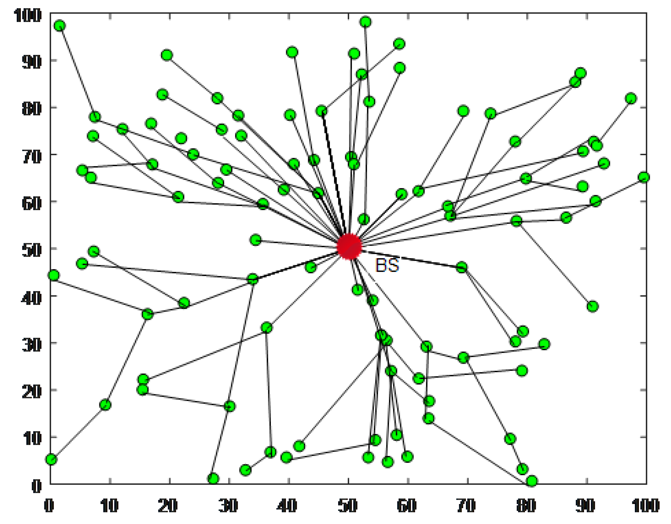
Figure 4 shows an example of data transmission path established by EBRA-NLE algorithm, where 100 nodes (i.e., network size N = 100) randomly distributed in 100 × 100 m2 monitoring area.
5.1. The Utilization of Energy
- (1)
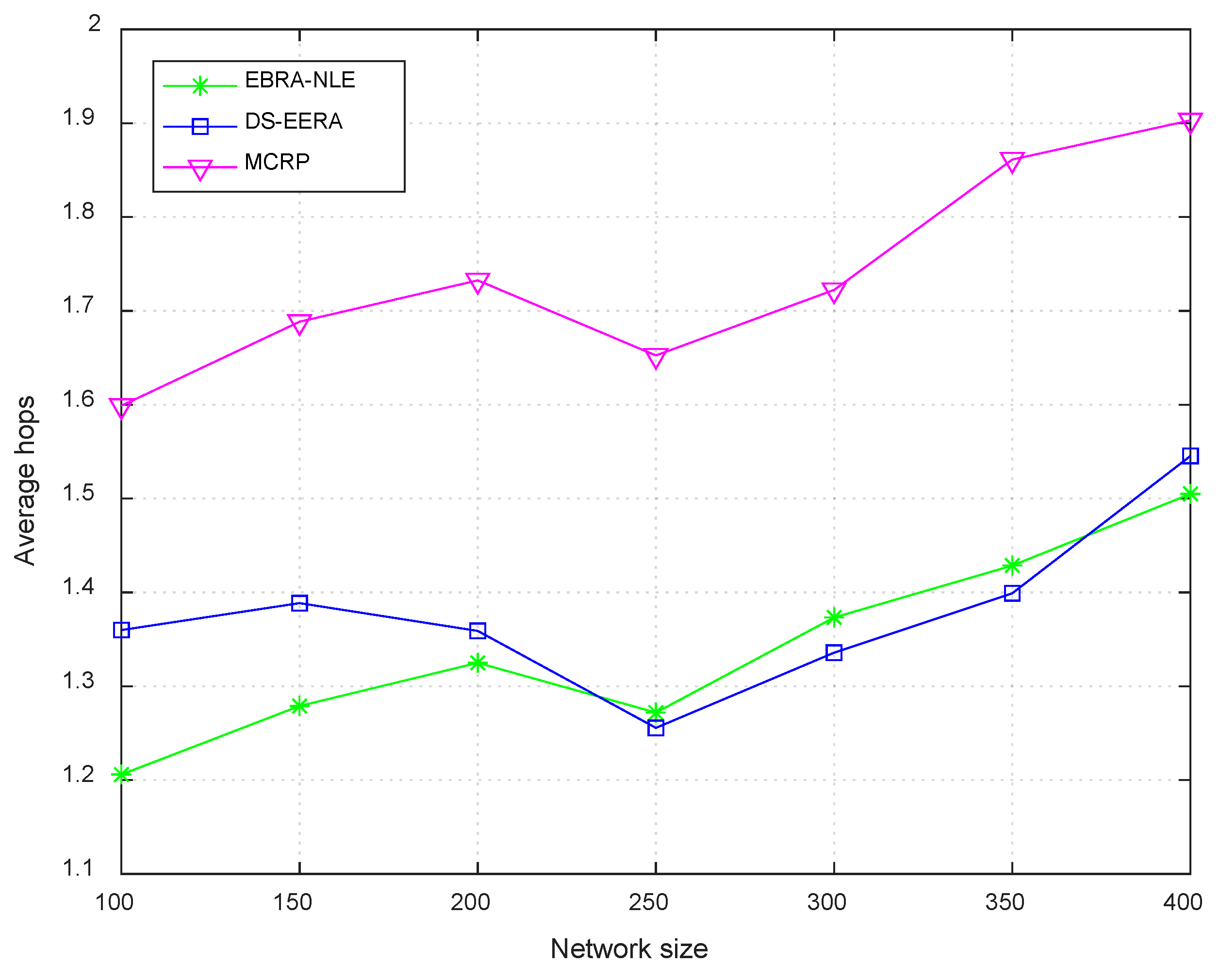
- The average hops
Figure 5 shows average hops with varying network size. It is shown that with the increase of network size, the average hops increases in the fluctuation. Obviously, the average hops of MCRP algorithm is the highest, DS-EERA and EBRA-NLE proposed in this paper are lower. This is because when choosing the next hop, EBRA-NLE and DS-EERA both consider the distance between the forward neighboring nodes and BS, and the closeness to the shortest path. In this paper, EBRA-NLE maps the indexes of nodes with sine function when establishing the belief function, which makes the belief function weighted according to the difference of index dimension, so that the advantage is more promising.
- (2)
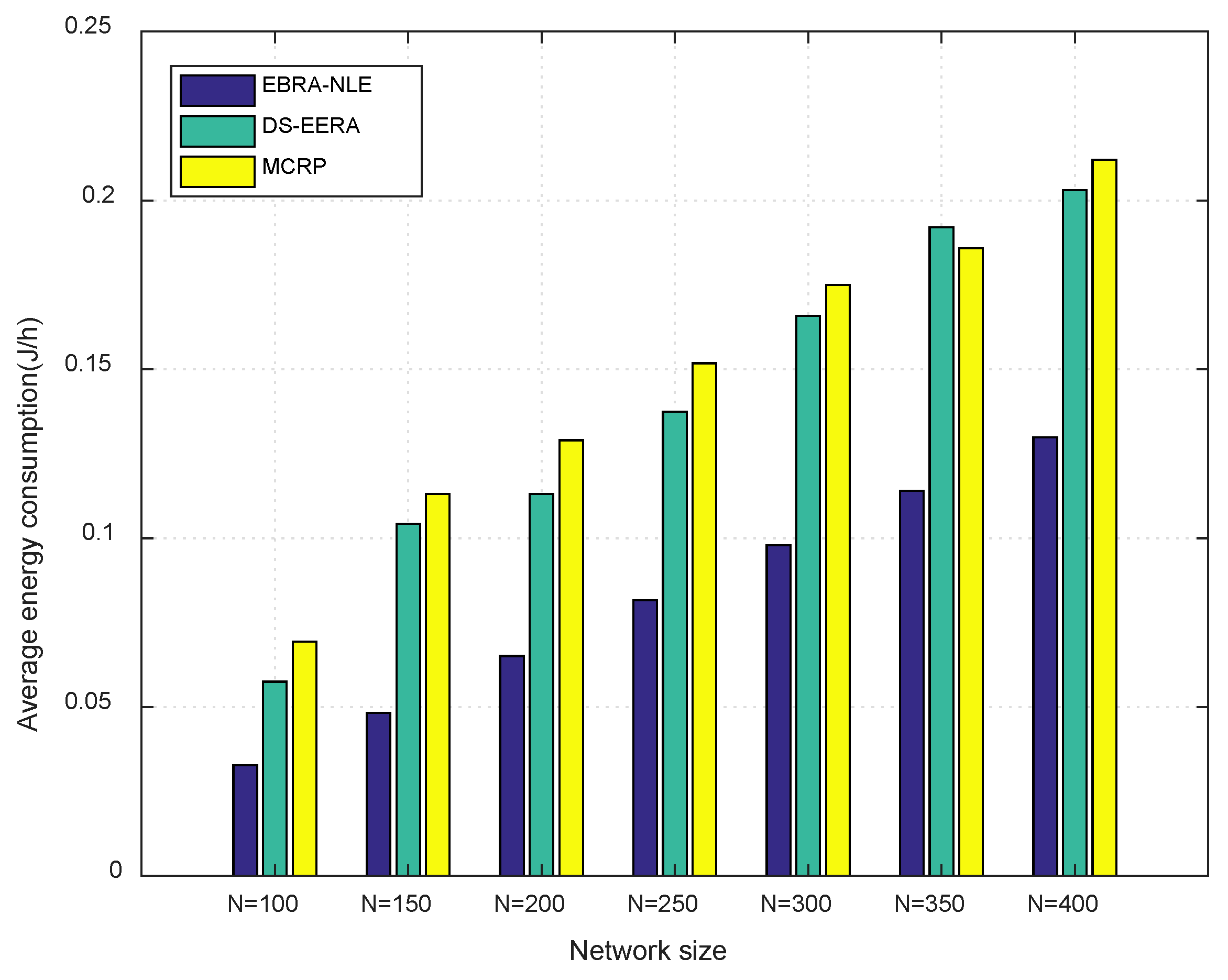
- Average energy consumption
Figure 6 shows the average energy consumption per hour in the whole network of the three algorithms under different network size. As can be seen from Figure 6, the average energy consumption of the three algorithms increases with the increase of the number of nodes in the network, and the EBRA-NLE proposed in this paper is always kept at the lowest level. First of all, the average energy consumption in the network will increase with the increase of the number of nodes, the average number of hops of EBRA-NLE is low, and the data transmission path is as close to the shortest path as possible, so it can effectively reduce the overall energy consumption of the network. Nevertheless, MCRP ignores the distance factor in route planning, which may lead to energy waste due to detours.
5.2. The Balance of Energy
- (1)
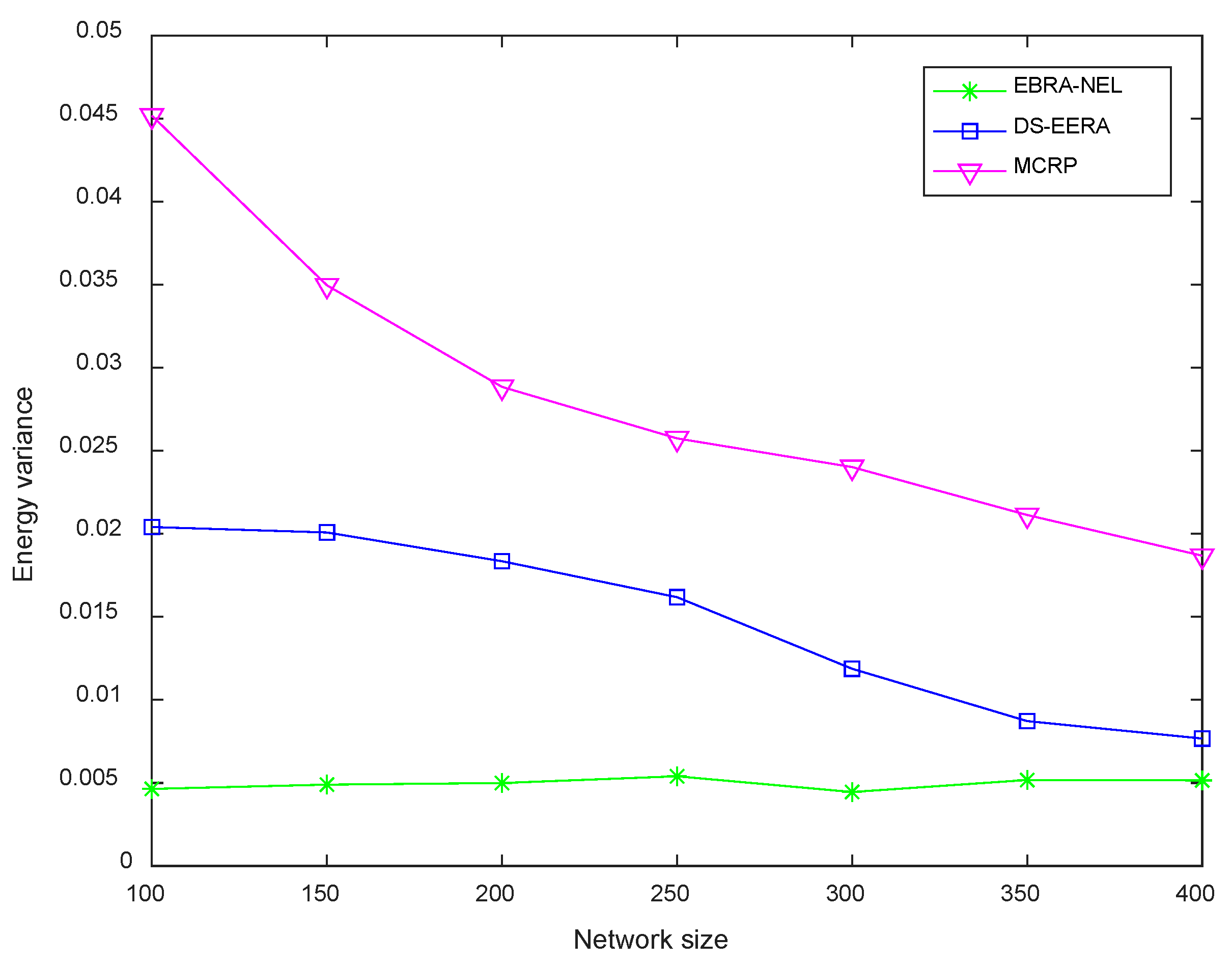
- Energy variance
Figure 7 shows the variance of residual energy of nodes in the network as the network size changes at the end of network operation of three algorithms. It can be seen that the energy balance of MCRP is poor, followed by DS-EERA. The energy balance of EBRA-NLE proposed in this paper is the proposing, and its energy variance is always kept at a low level under different network size. This is because in the decision-making indexes, “energy balance factor” and “buffer idleness” of EBRA-NLE consider the current energy and traffic of the forward neighbors, and send the data to the forward neighbor node with high energy and light load as the next hop. Therefore, the energy consumption between nodes is relatively balanced, and the network can work for a longer time.
- (2)
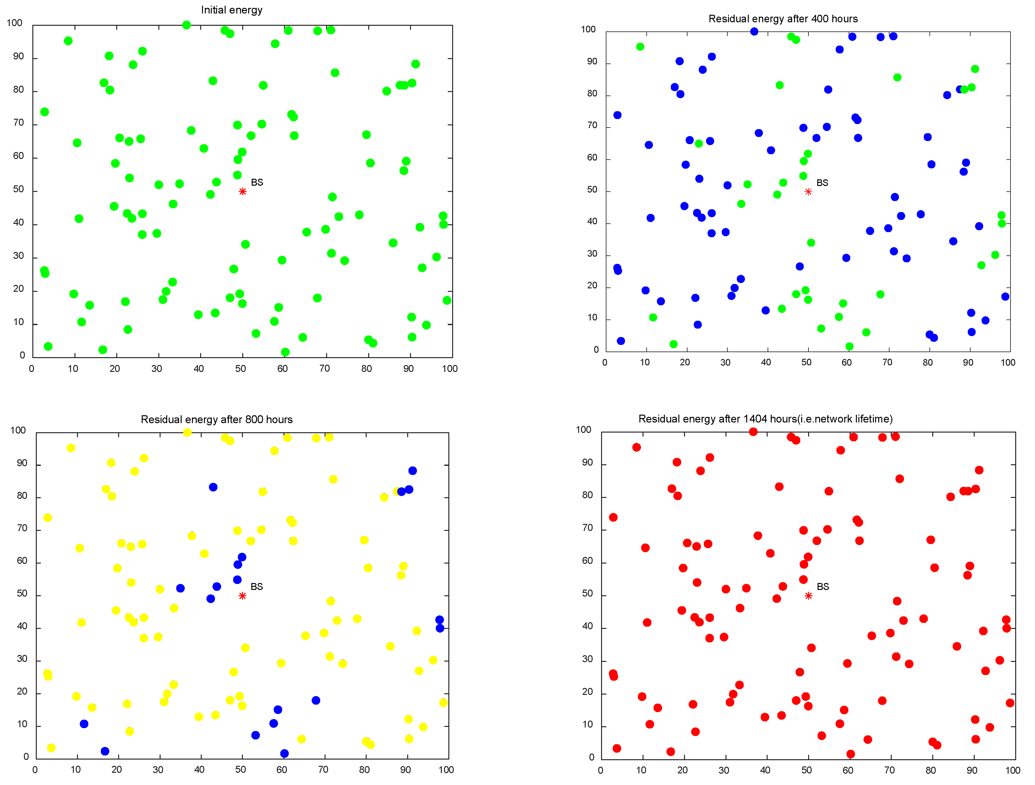
- Energy distribution
Figure 8 shows the distribution of the residual energy of nodes over time with 100 nodes randomly distributed in the monitoring area of 100 × 100 m2. The figure in the upper left shows the energy distribution at the initial moment of network operation, the energy of all nodes is full and equal. In the lower left, the network reaches its lifetime after 1404 h of network operation. It can be seen from the Figure 8 that the energy of the nodes in the network is consumed evenly over time, the residual energy between the nodes is balanced, and there is no energy hole problems.
- (3)
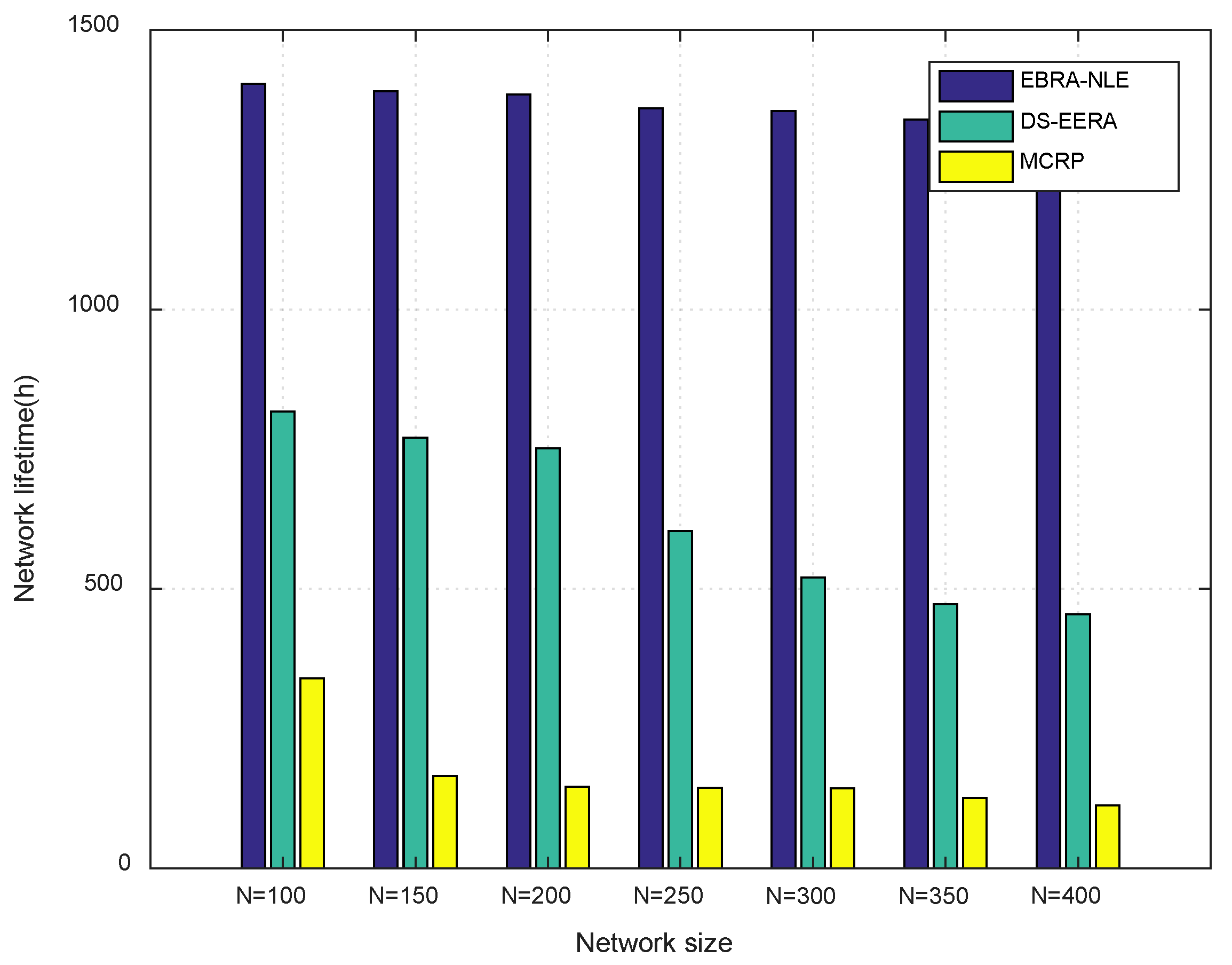
- Network lifetime
Figure 9 shows the comparison of the network lifetime of the three algorithms with the change of network size. It can be seen that the network lifetime of the EBRA-NLE proposed in this paper is always the highest, and is more than 50% higher than that of DS-EERA and MCRP in most cases. For example, when N = 100, the network lifetime of MCRP, DS-EERA, and EBRA-NLE is 340 h, 817 h, and 1404 h, which means that EBRA-NLE is improved about 313% and 72% more than that of MCRP and DS-EERA respectively. This is because according to Figure 7 and Figure 8, the energy of nodes in the data transmission path established by EBRA-NLE can be utilized in a balanced way. Meanwhile, according to Figure 6, the average energy consumption of EBRA-NLE is also low, and the energy consumption on the path during data transmission is less. So its energy efficiency is higher, and it can achieve a longer network operation time.
- (4)
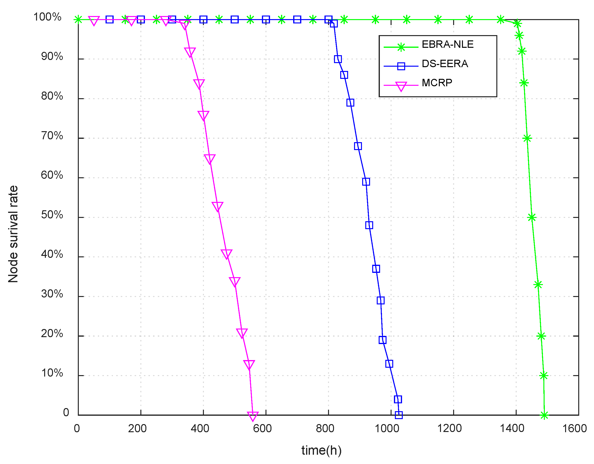
- Node survival rate
The survival rate of nodes in the network can also reflect the effectiveness and balance of energy utilization in a certain extent. Figure 10 shows the curve of node survival rate of three algorithms with varying time when the number of nodes in the network is 100. It can be seen that the first node death time of MCRP, DS-EERA, and EBRA-NLE is 340 h, 817 h, and 1404 h respectively. When all nodes in the MCRP and DS-EERA are dead, EBRA has not yet seen the first node death. Obviously, the curve of EBRA-NLE is the steepest, and that of MCRP is more smoothly after they reach their first node death. This is because the difference of residual energy between nodes in MCRP is large. When the first node in the network dies, the residual energy of other nodes is still sufficient, thus reaching the network lifetime prematurely. It is evident that the energy balance between the EBRA-NLE proposed in this paper is promising, which can effectively extend the network lifetime.
6. Conclusions
In this paper, in order to efficiently manage the energy of WSN-assisted IoT by considering energy balance and energy consumption minimization, a routing algorithm called energy balanced routing algorithm for network lifetime enhancement (EBRA-NLE) is proposed. Three attribute indexes are established as criterion to evaluate the forward neighboring nodes. Then we innovatively introduced a DS evidence theory-based routing algorithm to select the optimal routing path for each node. Simulation results assert the effectiveness of the proposed EBRA-NLE on enhancing the energy balance and network lifetime. The network lifetime obtained by EBRA-NLE is improved about 313% and 72% more than that of MCRP and DS-EERA algorithm respectively.
In future works, we aim to evaluate our proposed approach in the rechargeable sensor networks and combined with some energy harvest methods to further extend the network lifetime of WSN-assisted IOT.
Author Contributions
Conceptualization, L.T. and Z.L.; methodology, L.T. and Z.L.; software, Z.L.; validation, Z.L.; formal analysis, Z.L.; investigation, Z.L.; resources, L.T.; data curation, Z.L.; writing original draft preparation, Z.L.; writing—review and editing L.T.; visualization, Z.L.; L.T.; All authors have read and agreed to the published version of the manuscript.
Funding
This research was funded by the National Natural Science Foundation of China (No. 51677065).
Conflicts of Interest
The authors declare no conflict of interest.
References
- Floerkemeier, C.; Langheinrich, M.; Fleisch, E.; Mattern, F.; Sarma, S.E. The Internet of Things. Electron World 2017, 297, 949–955. [Google Scholar]
- Alhmiedat, T.; Taleb, A.A.; Bsoul, M. A study on threads detection and tracking systems for military applications using wsns. Int. J. Comput. Appl. 2012, 40, 12–18. [Google Scholar] [CrossRef]
- Aslan, Y.E.; Korpeoglu, I.; Ulusoy, O. A framework for use of wireless sensor networks in forest fire detection and monitoring. Comput. Environ. Urban Syst. 2012, 36, 614–625. [Google Scholar] [CrossRef]
- Nandurkar, S.; Thool, V.; Thool, R. Design and development of precision agriculture system using wireless sensor network. In Proceedings of the Automation Control Energy and Systems (ACES), Proceedings of First International Conference, Hooghly, West Bengal, India, 1–2 February 2014; pp. 1–6. [Google Scholar]
- Yan, J.; Zhou, M.; Ding, Z. Recent advances in energy-efficient routing protocols for wireless sensor networks: A review. IEEE Access 2016, 4, 5673–5686. [Google Scholar] [CrossRef]
- Chiang, S.; Huang, C.; Chang, K. A Minimum Hop Routing Protocol for Home Security Systems Using Wireless Sensor Networks; IEEE Press: New York, NY, USA, 2007; Volume 53, pp. 1483–1489. ISBN 1558-4127. [Google Scholar]
- Fei, L.; Chen, Y.; Gao, Q.; Peng, X.H. Energy hole Mitigation Through Cooperative Transmission in Wireless Sensor Networks. Int. J. Distrib. Sens. Netw. 2015, 2015, 1–14. [Google Scholar] [CrossRef] [Green Version]
- Xu, X.L. A Novel Transmission Range Adjustment Strategy for Energy Hole Avoiding in Wireless Sensor Network. J. Net. Compt. Appl. 2016, 67, 43–52. [Google Scholar]
- Zeng, Z.W.; Chen, Z.G.; Liu, A.F. Energy Hole Avoidance Based on Adjustable Transmission Power in Wireless Sensor Networks. Chin. J. Comput. 2010, 33, 12–22. [Google Scholar] [CrossRef]
- Xu, C.; Xiong, Z.Y.; Zhao, G.F.; Yu, S. An Energy-Efficient Region Source Routing Protocol for Lifetime Maximization in WSN; IEEE Access: New York, NY, USA, 2019; Volume 7, pp. 135277–135289. [Google Scholar]
- Shafer, G.A. A Mathematical Theory of Evidence; Princeton University Press: Princeton, NJ, USA, 1976. [Google Scholar]
- Ho, J.; Shih, H.; Liao, B.; Chu, S. A ladder diffusion algorithm using ant colony optimization for wireless sensor networks. Inf. Sci. 2012, 192, 204–212. [Google Scholar] [CrossRef]
- Falcon, R.; Hai, L.; Nayak, A.; Stojmenovic, I. Controlled straight mobility and energy-aware routing in robotic wireless sensor networks. In Proceedings of the IEEE Distributed Computing in Sensor Systems (DCOSS), Hangzhou, China, 16–18 May 2012; pp. 150–157. [Google Scholar]
- Bouabdallah, F.; Bouabdallah, N.; Boutaba, R. Efficient reporting node selection-based MAC protocol for wireless sensor networks. Wirel. Netw. 2013, 19, 373–391. [Google Scholar] [CrossRef]
- Behzadan, A.; Anpalagan, A.; Ma, B. Prolonging network lifetime via nodal energy balancing in heterogeneous wireless sensor networks. In Proceedings of the IEEE International Conference on Communications (ICC), Kyoto, Japan, 5 June 2011; pp. 1–5. [Google Scholar]
- Petrioli, C.; Nati, M.; Casari, P.; Zorzi, M.; Basagni, S. ALBA-R: Load-balancing geographic routing around connectivity holes in wireless sensor networks. IEEE Trans. Parallel Distrib. Syst. 2014, 25, 529–539. [Google Scholar] [CrossRef]
- Mehmmood, A.A.; Sarab, F.; Majed, A.-R.; Brajendra, K.S.; Kemal, E.T.; Rachid, B. Extending Wireless Sensor Network Lifetime With Global Energy Balance. IEEE Sens. J. 2015, 15, 5053–5063. [Google Scholar]
- Gupta, G.P.; Jha, S. Integrated clustering and routing protocol for wireless sensor networks using Cuckoo and Harmony Search based metaheuristic techniques. Eng. Appl. Atif. Intell. 2018, 68, 101–109. [Google Scholar] [CrossRef]
- Hajji, F.E.; Leghris, C.; Douzi, K. Adaptive Routing Protocol for Lifetime Maximization in Multi-Constraint Wireless Sensor Networks. J. Commun Inf. Netw. 2018, 3, 67–83. [Google Scholar] [CrossRef]
- Wang, X.; Li, D.; Zhang, X.; Cao, Y. MCDM-ECP: Multi Criteria Decision Making Method for Emergency Communication Protocol in Disaster Area Wireless Network. Appl. Sci. 2018, 8, 1165. [Google Scholar] [CrossRef] [Green Version]
- Khan, B.M.; Bilal, R.; Young, R. Fuzzy-TOPSIS Based Cluster Head Selection in Mobile Wireless Sensor Networks. J. Electr. Syst. Inf. Technol. 2017, 5, 928–943. [Google Scholar] [CrossRef]
- Tang, L.R.; Lu, Z.L.; Fan, B. Energy Efficient and Reliable Routing Algorithm for Wireless Sensors Networks. Appl. Sci. 2020, 10, 1885. [Google Scholar] [CrossRef] [Green Version]
- Lv, Y.H.; Liu, Y.; Hua, J.F. A Study on the Application of WSN Positioning Technology to Unattended Areas. IEEE Access 2019, 7, 38085–38099. [Google Scholar] [CrossRef]
- Luo, J.; Hu, J.Y.; Wu, D.; Li, R.F. Opportunistic Routing Algorithm for Relay Node Selection in Wireless Sensor Networks. IEEE. Trans. Ind. Inf. 2015, 11, 112–121. [Google Scholar] [CrossRef]
- Wang, Y.; Cheng, S.; Zhou, Y.; Peng, G.; Zhou, D.; Chao, C. Decision of air-to-air operation mode of airborne fire control radar based on DS evidence theory. Mod. Radar 2017, 39, 79–84. [Google Scholar]
- Zhu, D.Q.; Yang, Y.Q.; Yu, S.L. Dempster Shafer information fusion algorithm of electronic equipment fault diagnosis. Control. Theory Appl. 2004, 4, 659–663. [Google Scholar]
- Han, J.; Tao, Y.G. Data Fusion Algorithm of Multi sensor Based on D-S Evidential Theory and Fuzzy Mathematics Chinese Journal of Scientific. Chin. J. Sci. Instrum. 2000, 21, 644–647. [Google Scholar]
Figure 1.
The topology of wireless sensor networks (WSN).

Figure 2.
Distinguish routing process based on DS fusion rules.

Figure 3.
Sinusoidal mapping of membership function.

Figure 4.
Example of network routing path.

Figure 5.
The average hops with varying network size.

Figure 6.
The average energy consumption comparisons with varying network size.

Figure 7.
The energy variance with varying network size.

Figure 8.
The residual energy distribution of EBRA-NLE with different time when network size is N = 100. Where the red nodes denote that the residual energy percentage is [0, 25%], the yellow nodes denote that the residual energy is [25%, 50%], the blue nodes denote that the residual energy is [50%, 75%], and the green nodes denote that the residual energy is [75%, 100%].

Figure 9.
The network lifetime with varying network size.

Figure 10.
The node survival rate with varying time.


Table 1.
Simulation parameters.
| Definition | Value |
|---|---|
| Simulation area (L × L) | 100 × 100 m2 |
| Network size (N) | 100~400 |
| BS | (50,50) |
| Maximum communication radius (R) | 30 m |
| Packets size | 1024 bits |
| Buffer size | 20 packets |
| Initial energy () | 0.5 J |
| Data generation rate | 1024 bits~5120 bits/h |
© 2020 by the authors. Licensee MDPI, Basel, Switzerland. This article is an open access article distributed under the terms and conditions of the Creative Commons Attribution (CC BY) license (http://creativecommons.org/licenses/by/4.0/).
Share and Cite
MDPI and ACS Style
Tang, L.; Lu, Z. DS Evidence Theory-Based Energy Balanced Routing Algorithm for Network Lifetime Enhancement in WSN-Assisted IOT. Algorithms 2020, 13, 152. https://0-doi-org.brum.beds.ac.uk/10.3390/a13060152
AMA Style
Tang L, Lu Z. DS Evidence Theory-Based Energy Balanced Routing Algorithm for Network Lifetime Enhancement in WSN-Assisted IOT. Algorithms. 2020; 13(6):152. https://0-doi-org.brum.beds.ac.uk/10.3390/a13060152
Chicago/Turabian StyleTang, Liangrui, and Zhilin Lu. 2020. "DS Evidence Theory-Based Energy Balanced Routing Algorithm for Network Lifetime Enhancement in WSN-Assisted IOT" Algorithms 13, no. 6: 152. https://0-doi-org.brum.beds.ac.uk/10.3390/a13060152
Note that from the first issue of 2016, this journal uses article numbers instead of page numbers. See further details here.