Novel Graph Model for Solving Collision-Free Multiple-Vehicle Traveling Salesman Problem Using Ant Colony Optimization

Abstract

In this paper, a novel graph model to figure Collision-Free Multiple Traveling Salesman Problem (CFMTSP) is proposed. In this problem, a group of vehicles start from different nodes in an undirected graph and must visit each node in the graph, following the well-known Traveling Salesman Problem (TSP) fashion without any collision. This paper’s main objective is to obtain free-collision routes for each vehicle while minimizing the traveling time of the slowest vehicle. This problem can be approached by applying speed to each vehicle, and a novel augmented graph model can perform it. This approach accommodates not only the position of nodes and inter-node distances, but also the speed of all the vehicles is proposed. The proposed augmented graph should be able to be used to perform optimal trajectories, i.e., routes and speeds, for all vehicles. An ant colony optimization (ACO) algorithm is used on the proposed augmented graph. Simulations show that the algorithm can satisfy the main objective. Considered factors, such as limitation of the mission successfulness, i.e., the inter-vehicle arrival time on a node, the number of vehicles, and the numbers of vehicles and edges of the graph are also discussed.

1. Introduction

Distribution systems involving autonomous vehicles, such as automated guided vehicles (AGV), are an interesting research topic that continuously grows in the operational research area. Routing and scheduling have been dominating issues to explore. Particularly, in applications involving multiple vehicles, vehicle routing problem (VRP) and its variants are well-known approach to solve client services. Such problems are usually generalized by the traveling salesman problem (TSP) [1,2,3,4,5]. Many approaches to solve complexity in TSP are explored, such as min-k-SCCP [6,7,8,9].

In general, many scholars are focused on the minimization of cost, especially with regard to the required processing time [1,10,11,12,13,14,15]. However, in the modern distribution systems, other issues, such as collision, appear [11,14]. Particularly, for instance, in warehouses, cross-sections always exist in their layout. This condition leads to an unsafe situation caused by the high possibility of collision. Numerous researches have been reported, such as conflict-free routing for material handling vehicles [10,11,12,13,14] and distribution system [15,16,17,18]. Thus, this issue emerges in studies on avoiding collision scheduling. Mostly, artificial intelligence (AI)-based methods were proposed to solve the problem [1,14,15,16,17,18].

Based on our investigation, less of the publications address a problem of asymmetric TSP (ATSP). In this problem, an individual (vehicle, human, etc.) is required to travel from node-to-node on a not-fully connected graph, where each node can be visited only once by minimizing a given cost function. This type of problem was initially analyzed by a simple problem such as TSP, which has been explored for decades [15,16,18,19,20,21,22,23,24]. At the first appearance, this problem was overcome by simple computational techniques, such as the ascent method [19] or taboo parallel search method [20]. However, as more variations of TSP appeared, the use of these computational techniques is inadequate, especially because of great computational efforts. A particular complex variant of TSP is Multiple TSP (MTSP), which is proven as NP-hard [10,25,26,27]. In the MTSP, each node is allowed to be visited only once. Furthermore, the order of the routes of each agent is free of constraint. Consequently, this scenario leads to split routes, i.e., there is no intercepted route among agents. Several methods were proposed, i.e., Ant Colony Optimization (ACO) [17,27,28], Bee Colony Optimization (BCO) [18], neural network [21], branch-and-bound algorithm [13], and so forth.

We introduce a variant of MTSP called Collision-Free Multiple Traveling Salesman Problem (CFMTSP). Unlike the typical MTSP, this problem considers a particular case where more than one vehicle can visit the same node to establish some activities. Similar to single TSP, each vehicle has to visit all nodes only once. However, unlike the typical MTSP, each node is allowed to be visited by each vehicle only once, and for a time interval, only a vehicle can occupy the node. In CFMTSP, we consider the mission that all the vehicles must accomplish their own TSP. Our objective is to minimize the completion time of the slowest vehicle. A side-effect problem arises, i.e., collision avoidance at each visited node, especially which has more than one edge. Collision issues have appeared in numerous works [29,30,31,32,33,34,35,36]. The typical definition of collision considers only vehicle-to-vehicle distance [10,11,12,13,14,29]. Here, each vehicle has a “safety area” around its body that cannot be occupied by other vehicles. However, under particular motion directions, the safety area cannot guarantee the safety, since the vehicle moves faster than the minimum allowable speed toward another vehicle. This problem was coined in the work of Fraichard and Asama [30] by introducing an “inevitable collision states”, i.e., a set of configurations (position and direction) of a vehicle that makes the vehicle fail to avoid collision with any object. A successful development of the framework of predicting the collision was introduced in Reference [31], and is called the “reciprocal velocity obstacle”. This work defines “obstacle” in a more precise manner, by considering not only the position of the obstacle but also the velocity of the vehicle and the obstacle. Therefore, the collision time can be predicted [32,33,34,35,36].

The typical MTSP is mostly solved by utilizing a conventional graph model consisting of a set of nodes and a set of edges. However, such a graph model cannot be used to handle the issue of the collision, since the model only describes the information of position. In our work, we propose a novel graph model that contains information on position and speed options. Speed, together with node-to-node distance, is useful to determine the minimum arrival time difference between any two vehicles on a node, which in turn, can be used as a collision indicator. We assume that the safety area on each node corresponds to its minimum allowable arrival time difference. In order to find the optimal solution, we utilize an Ant Colony Optimization (ACO) algorithm on the proposed graph model, such that the solution is not only a sequence of visited nodes but also the speed that is applied for the node-to-node trip. The typical algorithm uses a single species of ant to find the optimal single vehicle’s route search. However, it is inadequate to use that single species to solve CFMTSP. Therefore, we propose multiple species of ants, as each ant represents a specific vehicle. The main feature of such an ACO algorithm is in the assumption that each ant only recognizes pheromone trails from other ants in the same species.

Based on the previous study, the problem that is similar to the CFMTSP has never been explored yet. The closest research was reported in References [13,37,38]. The research in Reference [13] focused on finding the route and speed for the Vehicle Routing Problem (VRP). However, this method uses an assumption of independent speed choice between any two edges, which is mechanically unrealistic because of the existence of acceleration constraints (see [36]). The issue of collision in MTSP appeared in References [37,38,39]. In Reference [37], a fleet of vehicles serves all nodes in an overlapped time-based batch. Accordingly, this problem may contain the possibility of collision, as well, since any two vehicles can visit the same node in an overlapped time. In Reference [38], a variant of TSP, namely Close Enough Traveling Salesmen Problem (CETSP), is presented. This work considers the node more as an area with a predetermined radius rather than the nodes as points. Moreover, the area is allowed to be occupied by only one vehicle at any time. However, similar to Reference [13], the node-to-node travel time in both articles is assumed to be predetermined. This assumption is practically not realistic, because a single (autonomous) vehicle is controlled automatically by a computer-based control system [39]. The control system has to send some speed instructions to the AGV while traveling some paths [35]. Several published algorithms did not consider speed selection, because they was assumed that some constant speeds are applied to the paths [25,26,27].

The organization of this paper is described as follows. Section 2 introduces several terminologies needed to support the analysis and discussions. Section 3 describes the problem statement. Section 4 explains the proposed methods, including the proposed augmented graph and the application of ACO on the graph. Section 5 reveals the simulation results and discussions. Finally, Section 6 concludes the overall work and describes future works.

2. Preliminaries

Let $G\left(V,E\right)$ be an undirected graph, where $V={\left\{v_{\mathrm{i}}\right\}}_{i=1}^{N_{\mathrm{v}}}$ denotes a set of $N_{\mathrm{v}}$ nodes, and $E=\left\{e_{i,j}\right\}$ is a set of edges connecting two nodes $v_i$ and $v_j$, i.e., $e_{i,j}=\left\{\left(v_i,v_j\right)|i, j \in \left\{1, 2,\dots ,N_{\mathrm{v}}\right\}\right\}$. In addition, let $B=\left\{b_{i,j}\right\}\in {\left\{0,1\right\}}^{N_{\mathrm{v}}\times N_{\mathrm{v}}}$ be an adjacency matrix of $G$, i.e., the matrix that describes the connectivity of any pair of nodes in $V$, where $b_{i,j}$ is assigned to one if $v_i$ and $v_j$, $i\ne j$, are connected and zero elsewhere. Let $S=\left\{s_l\right|l\in \left\{1, 2,\dots ,N_{\mathrm{s}}\right\}\}$ be a set of $N_{\mathrm{s}}$ speed options $s_l$ to be applied to all vehicles at any node in $G$. Suppose that there exists a group of $N_{\mathrm{u}}$ vehicles that are assigned to visit each node in $G$.

Definition 1.

Route and sub-route. A sub-route from $v_i$ to $v_j$ is defined as $e_{i,j}$, and a route is defined as a sequence of sub-routes, i.e., $\Xi =\left\{e_{i,j}|i, j \in \left\{1, 2,\dots ,N_v\right\}\right\}$ that begins from the start node $v_{i, start}\in V$ to the end node $v_{i,end}\in V$. The sub-route and route that are traveled by the k-th vehicle, $k\in \left\{1,\dots ,N_u\right\}$, are denoted as $e_{i,j}^k\in E$ and ${\Xi }^k$, respectively.

Definition 2.

Trajectory and sub-trajectory. A sub-trajectory ${\psi }_{i,j,l}$ is defined as a pair of sub-routes and speed option $\left(e_{i,j}, s_l\right)$, or in other words, the sub-route from the i-th node to the j-th node by applying the l-th speed option. A trajectory is a sequence of sub-trajectories, denoted as $\Psi =\left\{{\psi }_{i,j,l}\right\}$ connecting the start node $v_{i,start}\in V$ to the end node $v_{i,end}\in V$. The sub-trajectory and trajectory that are traveled by the k-th vehicle are denoted as ${\psi }_{i,j,l}^k$, and ${\Psi }^k$, respectively.

Definition 3.

Arrival time. Arrival time of the k-th vehicle to the i-th node, denoted as $t_i^k$, is defined as the time when the vehicle starts to enter the node.

Definition 4.

Operational time. The operational time of the k-th vehicle on the i-th node, denoted as $t_{op}$, is defined as the difference between the times the vehicle leaves and enters the node.

Definition 5.

Completion time. A completion time, $t_c^k$, is the time required by the k-th vehicle to visit all nodes in G.

Definition 6.

Collision. Any two vehicles are said to have not collided at the i-th node if, and only if, the arrival time difference $\left|t_i^{k_1}-t_i^{k_2}\right|>t_{op}$, $k_1\ne k_2$, and during the time interval each vehicle is out in the inevitable collision states defined in References [21,22].

3. Problem Statement

In this study, we enhanced the problem of the typical TSP (see [6,12]) to collision-free multiple TSP (CFMTSP). In this problem, each vehicle attempts to establish its individual TSP mission. The CFMTSP is described as follows. First, we need to find a complete trajectory for all vehicles, i.e., $\left\{{\psi }_{\mathrm{i},\mathrm{j},\mathrm{l}}^{\mathrm{k}}\right\}$, such that the following function is minimized:

$$t_{\max }=\max \left(t_c^1,t_c^2,\dots ,t_c^{N_{\mathrm{u}}}\right),$$

(1)

subject to the following:

• There is no collision between any vehicles (see Definition 6) at each node.
• The start times, $t_{\mathrm{start}}^k$, of all vehicles are zero, i.e., $t_{\mathrm{start}}^1=t_{\mathrm{start}}^2=\dots =t_{\mathrm{start}}^{N_{\mathrm{u}}}=0$.
• $s_l>0$.

Note that the second constraint is designated to be a collision indicator. If the constraint is violated, then the vehicles have collided with each other. The third constraint emphasizes that there is no delay among the start times of the vehicles.

Assumption 1.

All vehicles start from different nodes.

Assumption 2.

The operational times, $t_{op}$, for all nodes in Gare assumed to be constant.

Assumption 3.

The number of speed options, i.e., $N_s$, is the same for all vehicles.

Assumption 4.

Collisions are considered only at the nodes. The edges are assumed to be sufficiently broad, so that any vehicles passing through the same edge will not collide with each other.

Assumption 5.

The graph $G\left(V,E\right)$ is not a multi-graph, i.e., the number of edges between any two nodes is exactly one.

4. Proposed Methods

4.1. Augmented Graph

4.1.1. Graph Model

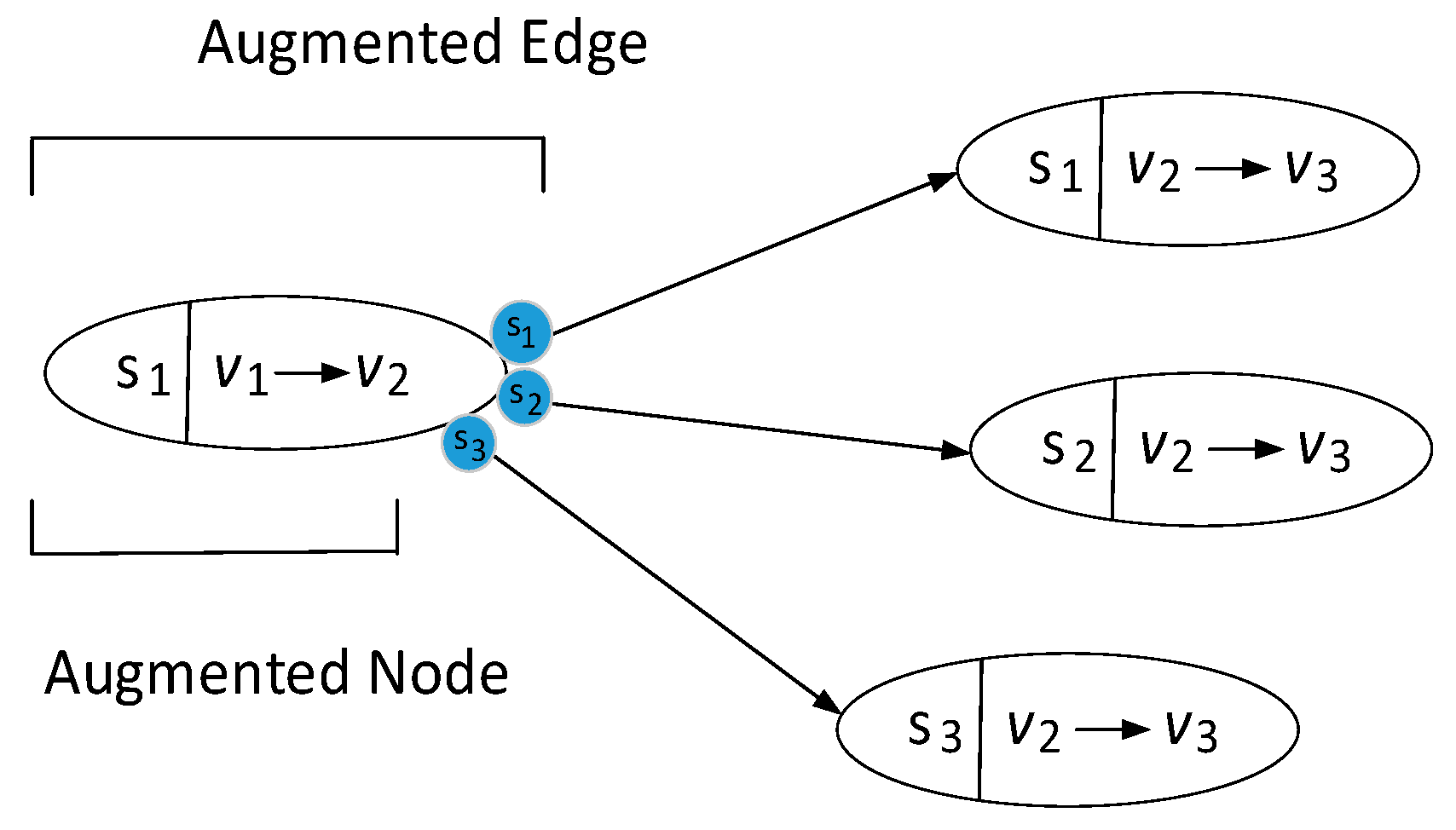
Solving the problem described in (1) is difficult by using typical graph $G$, since there is no information about the arrival time of each vehicle at each node. Consequently, the inter-vehicle collision problem is unable to solve. To address such a problem, instead of using typical graph $G$, we developed a novel structure of the graph, which is called an augmented graph, denoted by $G^{\mathrm{a}}$. The augmented node can be constructed from the typical graph $G$. Let $G^{\mathrm{a}}\left(V^{\mathrm{a}}, E^{\mathrm{a}}\right)$ be an augmented graph, where $V^{\mathrm{a}}=\left\{{\psi }_{i,j,l}\right\}$, as long as $b_{i,j}=1$, $i, j \in \left\{1,\dots ,N_{\mathrm{v}}\right\}$ and $l\in \{1,2,\dots ,N_{\mathrm{s}}$}, is defined as a set of augmented nodes and $E^{\mathrm{a}}=\left\{{\xi }_{i_1,j_1,l_1}^{i_2,j_2,l_2}\right\}$, where ${\xi }_{i_1,j_1,l_1}^{i_2,j_2,l_2}=\left({\psi }_{i_1,j_1,l_1}, {\psi }_{i_2,j_2,l_2}\right)$ is augmented edge, i.e., start and end connected sub-trajectories pairs ${\psi }_{i_1,j_1,l_1}$ and ${\psi }_{i_2,j_2,l_2}$. Note that the notation ${\xi }_{i_1,j_1,l_1}^{i_2,j_2,l_2}$ implies that ${\psi }_{i_2,j_2,l_2}$ must be a successor of ${\psi }_{i_1,j_1,l_1}$. Therefore, it is required that $i_2=j_1$.

Figure 1 visualizes the proposed $G^{\mathrm{a}}$, $V^{\mathrm{a}}$, and $E^{\mathrm{a}}$. $G^{\mathrm{a}}$ expands the typical $G$ from the node-to-node relation into transition-to-transition relation. In the typical graph $G$, the edges are weighted by node-to-node distance $L_{i,j}$ while in the augmented graph $G^{\mathrm{a}}$, the augmented edges are weighted by acceleration, whose formulation is conducted using start and final speeds the node-to-node distance (see Equation (5)).

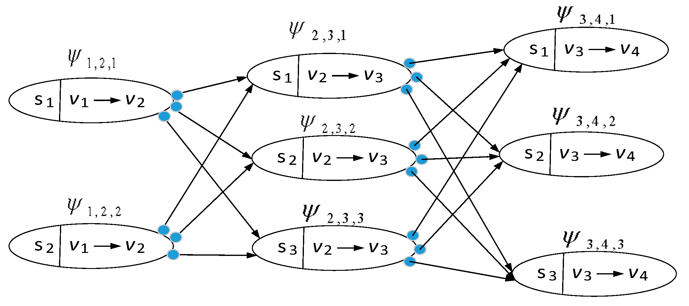
Figure 2 shows that, for a node-to-node trajectory, there are some speed alternatives to apply. Therefore, the augmented edge between any pair of augmented nodes can represent information of acceleration and traveling time, for instance, the transition from ${\psi }_{1,2,1}$ to ${\psi }_{2,3,2}$. The applied initial and target speeds at the endpoint of ${\psi }_{1,2,1}$ are $s_1$ and $s_2$, respectively. Therefore, the uniform acceleration $a_{1,2}$ along the augmented edge is formulated as following:

$$a_{i,j}=\frac{{\left(s_j\right)}^2-{\left(s_i\right)}^2}{2L_{i,j}},$$

(2)

where $L_{i,j}$ is the length of the edge ${\mathrm{e}}_{1,2}$, and it is plotted to the transition from ${\psi }_{1,2,1}$ to ${\psi }_{2,3,2}$.

Furthermore, the traveling time, $t$, related to the acceleration in Equation (2) is formulated as follows:

$$t=\{\begin{array}{c}\frac{L_{i,j}}{s_i}, \mathrm{if} a=0, \\ \frac{-s_i+\sqrt{{\left(s_i\right)}^2+2a{L}_{i,j}}}{a_{i,j}}, \mathrm{otherwise}.\end{array}$$

(3)

4.1.2. Additional Adjacency Matrix

We introduced some supporting matrices to support the proposed algorithm. First of all, we introduced edge matrix, denoted as ${}_{}{}^{\mathrm{e}}B=\left\{{}_{}{}^{\mathrm{e}}b{}_{i,j}|i,j\in \left\{1,2,\dots ,N_{\mathrm{v}}\right\}\right\}$, whose dimension is the same with the adjacency matrix $B$. Let ${}_{}{}^{q}e$, where q is the identifier of an edge whose value can be determined by Algorithm 1, be defined as the edge identifier of each element of $B$, i.e., $b_{i,j}$ that has the value of 1. Therefore, we get the following:

$${}_{}{}^{\mathrm{e}}b{}_{i,j}=\{\begin{array}{c}{}_{}{}^{q}e, \mathrm{if} b_{i,j}>1,\\ 0, \mathrm{otherwise}.\end{array}$$

(4)

where $i,j\in \left\{1,2,\dots ,N_{\mathrm{v}}\right\}$.

Algorithm 1 Determine the index of edge matrix

1: Input: B

2: $q=0$;

3: For $i=1$ to $N_{\mathrm{v}}$

4:  For $j=1$ to $N_{\mathrm{v}}$

5:   If $i\ne j$ and $b_{i,j}=1$, then q = q +1 and ${}_{}{}^{q}e=q$.

6:  End

7: End

8: Output: all $\left\{{}_{}{}^{q}e\right\}$.

For instance, suppose that we have the following adjacency matrix of a graph $G$ whose number of nodes is 5, as follows.

$$B=\left[\begin{array}{ccc}\begin{array}{cc}\begin{array}{cc}\begin{array}{c}\begin{array}{c}\begin{array}{c}0\\ 0\\ 1\end{array}\\ 0\end{array}\\ 0\end{array}& \begin{array}{c}\begin{array}{c}\begin{array}{c}1\\ 0\\ 0\end{array}\\ 1\end{array}\\ 1\end{array}\end{array}& \begin{array}{c}\begin{array}{c}\begin{array}{c}0\\ 1\\ 0\end{array}\\ 1\end{array}\\ 1\end{array}\end{array}& \begin{array}{c}\begin{array}{c}\begin{array}{c}1\\ 0\\ 1\end{array}\\ 0\end{array}\\ 1\end{array}& \begin{array}{c}\begin{array}{c}\begin{array}{c}0\\ 0\\ 0\end{array}\\ 0\end{array}\\ 0\end{array}\end{array}\right]$$

(5)

Therefore, by using (4), we have the following:

$${}_{}{}^{\mathrm{e}}B=\left[\begin{array}{ccc}\begin{array}{cc}\begin{array}{cc}\begin{array}{c}\begin{array}{c}\begin{array}{c}0\\ 0\\ {}_{}{}^{4}e\end{array}\\ 0\end{array}\\ 0\end{array}& \begin{array}{c}\begin{array}{c}\begin{array}{c}{}_{}{}^{1}e\\ 0\\ 0\end{array}\\ {}_{}{}^{6}e\end{array}\\ {}_{}{}^{8}e\end{array}\end{array}& \begin{array}{c}\begin{array}{c}\begin{array}{c}0\\ {}_{}{}^{3}e\\ 0\end{array}\\ {}_{}{}^{7}e\end{array}\\ {}_{}{}^{9}e\end{array}\end{array}& \begin{array}{c}\begin{array}{c}\begin{array}{c}{}_{}{}^{2}e\\ 0\\ {}_{}{}^{5}e\end{array}\\ 0\end{array}\\ {}_{}{}^{10}e\end{array}& \begin{array}{c}\begin{array}{c}\begin{array}{c}0\\ 0\\ 0\end{array}\\ 0\end{array}\\ 0\end{array}\end{array}\right]$$

(6)

.

Furthermore, we use the index of ${}_{}{}^{q}e$, i.e., $q$ as the index of row of another adjacency matrix named trajectory adjacency matrix, denoted as ${}_{}{}^{\psi }B$. Each row and each column of this matrix represent edge ${}_{}{}^{q}e$ and speed $s_l$, respectively. Let ${}_{}{}^p\psi$ be the element of ${}_{}{}^{\psi }B$, where we have the following:

$$p\left(q,l\right)=\left(q-1\right)N_s+l ,$$

(7)

$l\in \left\{1,2,\dots ,N_{\mathrm{s}}\right\}$ and $q$ are defined in (4). Suppose that we apply three-speed options; therefore, $N_{\mathrm{s}}=3$. From the adjacency matrix example in Equation (5) and its respective edge matrix in (6), we have the elements of $T$ as follows: For edge ${}_{}{}^{1}e$, we have three trajectories, i.e., ${}_{}{}^1\psi$, ${}_{}{}^2\psi$, and ${}_{}{}^3\psi$. Since from Equations (5) to (7), ${}_{}{}^{1}e$ represents $e_{1,2}$, then ${}_{}{}^1\psi$, ${}_{}{}^2\psi$, and ${}_{}{}^3\psi$ represent ${\psi }_{1,2,1}$, ${\psi }_{1,2,2}$, and ${\psi }_{1,2,3}$, respectively. Similarly, ${}_{}{}^{5}e$ represents $e_{3,4}$. By using (10), we have trajectories ${}_{}{}^{13}\psi$, ${}_{}{}^{14}\psi$, and ${}_{}{}^{15}\psi$. Therefore, according to Equations (5)–(7), ${}_{}{}^{13}\psi$, ${}_{}{}^{14}\psi$, and ${}_{}{}^{15}\psi$ represent ${\psi }_{3,4,1}$, ${\psi }_{3,4,2}$, and ${\psi }_{3,4,3}$, respectively.

The last adjacency matrix is the augmented-edge adjacency matrix, denoted by ${}_{}{}^{\xi }B$, where the row and column are indexed by the index of ${}_{}{}^p\psi$, i.e., $p$. Let ${}_{}{}^h\xi$ be the element of ${}_{}{}^{\xi }B$, whose value is not zero and be associated to ${\xi }_{i_1,j_1,l_1}^{i_2,j_2,l_2}$ by applying Algorithm 2.

Algorithm 2 Determining the index of $\xi$:

1: Inputs: ${}_{}{}^{\psi }B, p_1,p_2$

2: Output: ${}_{}{}^{\xi }B$, ${}_{}{}^h\xi$

3: h = 0

4: For i = 1,…,$\left|{}_{}{}^{\psi }B\right|$// loop for all rows

5:  For j=1,…,$\left|{}_{}{}^{\psi }B\right|$  // loop for all columns

6:   $c_1$ = $ro{w}_{\psi }\left({}_{}{}^i\psi \right)$; $c_2$=$ro{w}_{\psi }\left({}_{}{}^j\psi \right)$

7:   If $c_1\ne c_2$

8:    If $en{d}_{\mathrm{e}}\left({}_{}{}^{c_1}e\right)$ = $star{t}_{\mathrm{e}}\left({}_{}{}^{c_1}e\right)$

9:     h=h+1

10:     ${}_{}{}^{\xi }b{}_{i,j}=h$

11:     ${}_{}{}^h\xi =h$

12:    Else

13:     ${}_{}{}^{\xi }b{}_{i,j}=0$

14:    End

15:   Else

16:    ${}_{}{}^{\xi }b{}_{i,j}=0$

17:   End if

18:  End for

19: End for

The functions $ro{w}_{\psi }\left(x\right)$, $star{t}_{\mathrm{e}}\left(x\right)$, and $en{d}_{\mathrm{e}}\left(x\right)$ return the row index belonged to the row in ${}_{}{}^{\psi }B$ containing x, the indexes of start and end node in ${}_{}{}^{\mathrm{e}}B$, respectively. In the previous example, there are ten edges and three speed options. The number of trajectories is 30 and the dimension of ${}_{}{}^{\xi }B={\mathbb{Z}}^{30\times 30}$. Until this step, we have the following adjacency matrices:${}_{}{}^{\mathrm{e}}B$, ${}_{}{}^{\psi }B$, and ${}_{}{}^{\xi }B$. Suppose that we are given ${}_{}{}^h\xi$; then, by using the map described in ${}_{}{}^{\xi }B$, we obtain ${}_{}{}^{p_1}\psi$ and ${}_{}{}^{p_2}\psi$, where $p_1$ and $p_2$ are the indexes of the row and column of ${}_{}{}^{\xi }B$ associated to ${}_{}{}^h\xi$. After that, we check the map in ${}_{}{}^{\psi }B$, and we obtain the edge ${}_{}{}^{q}e$ and speed option $s_l$ for each ${}_{}{}^{p_1}\psi$ and ${}_{}{}^{p_2}\psi$.

4.2. Ant Colony Optimization

Ant Colony Optimization (ACO) was first introduced in Reference [28]. This algorithm is powerful for routing problems such as traveling salesman problem (TSP), vehicle routing problem (VRP), and their variants [17,27]. The algorithm mimics the behavior of a colony of ants in foraging activities. Suppose that, at the beginning, the colony has no information about the location of the food source. An ant system (AS) consists of a set of artificial ants which perform foraging activities, from their nest to a food source. Some ants begin to move randomly to any direction and deposit a chemical called “pheromone”, whose trails will be traced by other ants. This process is iterated such that the optimal route is that with the maximum number of pheromone trails.

In this study, we used an ACO algorithm for finding trajectories for a multiple-vehicle system. The algorithm is different from the typical ones. It involves more than one species of ants whose pheromone the others cannot detect trails of. In the cases of CFMTSP, a species represents a vehicle. We develop an algorithm such that each species performs a collision-free trajectory, i.e., all species can prevent collision with each other. In this study, we assume that any two species are not colliding with each other if the difference of their arrival times exceeds a minimum allowable value.

Suppose that there exist $N_{\mathrm{u}}$ ant species. Each species consists of $N_{\mathrm{m}}$ ants. The r-th ant of the k-th species, denoted by ${\theta }^{k,r}$, $k\in \{1,2,\dots ,N_{\mathrm{u}}\}$, $r\in \left\{1,2,\dots ,N_{\mathrm{m}}\right\}$, represents the k-th vehicle. Each ant is assumed to be able to recognize only the trails produced by ants of the same species. Therefore, if there exists a large concentration of pheromone in a sub-route, if it comes from different species, then it is less possible for the ant to choose that sub-route as a choice. As the typical ACO algorithms, as one ant passes a sub-route, it leaves pheromone trails along the sub-routes. From now on, the others will smell the trails, and based on the largest amount of pheromones, it will choose the sub-route. Even though there are pheromones produced by other different ant species, the ant cannot recognize them. This behavior is similar to the behavior of some colonies of ants in the real world, that is, they cannot recognize the trail of other different ant species, as reported in Reference [40]. Researchers in that study have discovered that a species of ants, i.e., Lasius nigers (La. nigers), is unable to recognize the pheromone trails produced by Novomessor cockerelli (N. cockerelli) and Linepithema humilis (Li. humilis). The reason is that their pheromone trails are constructed by different chemicals.

In this model, we applied the amount of pheromone applied to the proposed augmented graph $G^{\mathrm{a}}$ to augmented edges ${}_{}{}^h\xi$. Define $n$, ${}_{}{}^h\tau {}^k$, and $\mathsf{\Delta }{}_{}{}^h\tau {}^{k,r}$ as the iteration, the total amount of pheromone left by the k-th ant species on augmented edges ${}_{}{}^h\xi$, and the increase of pheromone amount left by each r-th ant of the k-th ant species, respectively. We formulate ${}_{}{}^h\tau {}^k$ as follows.

$${}_{}{}^h\tau {}^k\left(n\right)={}_{}{}^h\tau {}^k\left(n-1\right)+{\displaystyle \sum }_{r=1}^{N_{\mathrm{m}}}\mathsf{\Delta }{}_{}{}^h\tau {}^{k,r}\left(n\right),$$

(8)

if a solution is found and the i-th and j-th nodes are the part of the augmented edge passed through by the k-th ant species, and

$${}_{}{}^h\tau {}^k\left(n\right)=\rho {}_{}{}^h\tau {}^k\left(n-1\right),$$

(9)

where $\rho ϵ (0,1]$ is defined as evaporation rate, if the search fails to find a solution. Furthermore, $\mathsf{\Delta }{}_{}{}^h\tau {}^{k,r}$ is formulated as follows:

$$\mathsf{\Delta }{}_{}{}^h\tau {}^{k,r}=\frac{Q}{d^{k,r}},$$

(10)

where $d^{k,r}$ is the total distance traveled by the r-th ant from the k-th species, and $Q$ is a positive constant.

We apply the probability of selecting ${}_{}{}^h\xi$, i.e., $Pr({}_{}{}^h\xi )$ as follows:

$$Pr({}_{}{}^h\xi )=\frac{{\left({}_{}{}^h\eta \right)}^{\beta }{\left({}_{}{}^h\tau {}^k\right)}^{\gamma }}{{{\displaystyle \sum }}_{all {}_{}{}^{h_i}\xi ϵ{\rm N}eighbors\left({}_{}{}^h\xi \right)}{\left({}_{}{}^{h_i}\eta \right)}^{\beta }{\left({}_{}{}^{h_i}\tau {}^k\right)}^{\gamma }},$$

(11)

Note that the selection of trajectories of more than one vehicle leads to a consequence of inter-vehicle collision-checking. Therefore, a procedure for checking the collision is developed.

Before describing the main algorithm, we define a number of variables: $v_{i,\mathrm{start}}^{k,r}$ and $s_{\mathrm{start}}^{k,r}$ are the initial position and speed, respectively. $L_{\mathrm{unv}}^k$, $L_{\mathrm{e}}^k$, $L_{\psi }^k$, $L_{\xi }^k$, and $L_{\xi ,\mathrm{sel}}^k$ are the lists of unvisited nodes, collection of edges, collection of trajectories, and collection of augmented-edges, the sequence of selected augmented-edges from the start to end nodes, respectively. $L_{\mathrm{vis}}^i$ is a collection for each node $i\in \left\{1,2,\dots ,N_{\mathrm{v}}\right\}$ that stores information of the k-th vehicle that has visited the node and its associated arrival time, $t_i^k$. ${\Psi }_{\mathrm{best}}^k$ is the best trajectory performed by the k-th species.

In Line 1 of Algorithm 3, the input is the graph $G$, initial positions $v_{i,\mathrm{start}}^{k,r}$, and speed $s_{\mathrm{start}}^{k,r}$ of each r-ant of the k-th ant species. Note that r also represents the index of iteration. Consequently, $N_{\mathrm{m}}$ represents the number of iterations. In Lines 3 and 4, all the required adjacency matrices are constructed, and $L_{\mathrm{unv}}^k$ for all ant species is set to be empty.

The searching process starts from Line 5. For each iteration, trajectories are constructed for each species. In Line 7, some required initializations are performed, such as the initial amount of pheromones. The values are set randomly small to prevent division-by-zero at the beginning at the process. The next processes are focused on identifying the augmented edge of the current occupied node, $v_{\mathrm{curr}}^k$.

The function CreateEdgeList($v_{\mathrm{curr}}^k$) is purposed to extract all edges ${}_{}{}^{q}e$ in $G$ whose start nodes are $v_{\mathrm{curr}}^k$. In this process, the edge matrix ${}_{}{}^{\mathrm{e}}B$ is used. The resulted ${}_{}{}^{q}e$ is then pushed to $L_{\mathrm{e}}^k$.

The next step is to extract the sub-trajectories, ${}_{}{}^p\psi$, whose edges are ${}_{}{}^{q}e$. However, two conditions make the extraction fail. First, it is possible that the end node of the edge ${}_{}{}^{q}e$, i.e., $en{d}_{\mathrm{e}}\left({}_{}{}^{q}e\right)$), was visited. Therefore, the availability of the end node of the edge must be checked (Line 13). Second, even though $en{d}_{\mathrm{e}}\left({}_{}{}^{q}e\right)$) is available, if there exists another ant occupying the node such that the second constraint is violated, then the process is continued to the next edge. This process is revealed in Lines 14–16.

If the end node of the edge ${}_{}{}^{q}e$ has not been visited yet and has no collision issue, then the function CreateTrajectoriesList($L_{\mathrm{e}}^k$, ${}_{}{}^{q}e$) is executed (Line 18). The CreateTrajectoriesList($L_{\mathrm{e}}^k$, ${}_{}{}^{q}e$) uses trajectory adjacency matrix ${}_{}{}^{\psi }B$ as reference to find the correct trajectories that are spanned by the q-th edge in $L_{\mathrm{e}}^k$. If the end node of the edge ${}_{}{}^{q}e$ has been visited previously, the process will check the other edges. If there is no edge available, then it can be concluded that a complete trajectory is failed to found. Therefore, the process is continued to new iteration (Lines 29–32). In Line 30, the amount of pheromone trails is reduced by calling ReducePheromoneTrailsAmount($L_{\xi }^k, {}_{}{}^h\tau {}^k$), which applies Equation (12).

Algorithm 3 Main Algorithm

1: Inputs: $G$, $v_{i,\mathrm{start}}^{k,r}$, $s_{\mathrm{start}}^{k,r}$, for all $k\in \left\{1,2,\dots ,N_{\mathrm{u}}\right\}$,$r\in \left\{1,2,\dots ,N_{\mathrm{m}}\right\}$,

2: Perform $,{}_{}{}^{\mathrm{e}}B$, ${}_{}{}^{\psi }B$, and ${}_{}{}^{\xi }B$.

3: ${\Psi }_{\mathrm{best}}^k\underset{}{\leftarrow }\{ \}$, for all $k\in \left\{1,2,\dots ,N_{\mathrm{u}}\right\}$.

4: $L_{\mathrm{unv}}^k\underset{}{\leftarrow }{\{ \}}_{i=1}^{N_{\mathrm{v}}}$, for all $k\in \left\{1,2,\dots ,N_{\mathrm{u}}\right\}$.

5: For r = 1 to $N_{\mathrm{m}}$

6: $v_{\mathrm{curr}}^k=v_{i,\mathrm{start}}^{k,r}$

7: Initialize($v_{\mathrm{curr}}^k$, $s_{\mathrm{start}}^{k,r}$);

8: $L_{\mathrm{unv}}^k\underset{}{\leftarrow }{\left\{v_i\right\}}_{i=1}^{N_{\mathrm{v}}}$, $L_{\mathrm{e}}^k\underset{}{\leftarrow }\{ \}$, $L_{\psi }^k\underset{}{\leftarrow }\{ \}$, $L_{\xi }^k\underset{}{\leftarrow }\{ \}$, $L_{\xi ,\mathrm{sel}}^k\underset{}{\leftarrow }\{ \}$, $L_{\mathrm{vis}}^i\underset{}{\leftarrow }\{ \}$.

9: For each k-th ant species

10:  While $L_{\mathrm{unv}}^k\ne \{ \}$

11:   $L_{\mathrm{e}}^k\underset{}{\leftarrow }$CreateEdgeList($v_{\mathrm{curr}}^k$).

12:   For each edge in $L_{\mathrm{e}}^k$, i.e., ${}_{}{}^{q}e$,

13:    If $en{d}_{\mathrm{e}}\left({}_{}{}^{q}e\right)\in L_{\mathrm{unv}}^k$,

14:     If IsCollided($L_{\mathrm{vis}}^i$, $en{d}_{\mathrm{e}}\left({}_{}{}^{q}e\right)$) is TRUE

15:      continue;

16:     End

17:     ${}_{}{}^p\psi =$ CreateSubTrajectoriesList($L_{\mathrm{e}}^k$,${}_{}{}^{q}e$).

18:     $L_{\psi }^k\underset{}{\leftarrow }{}_{}{}^p\psi$.

19:     For each p-th trajectory in $L_{\psi }^k$ i.e., ${}_{}{}^p\psi$,

20:      $L_{\xi }^k\underset{}{\leftarrow }$CreateAugmentedEdgesList($L_{\psi }^k$, ${}_{}{}^p\psi$).

21:     End

22:     $L_{\xi ,\mathrm{sel}}^k\underset{}{\leftarrow }$SelectAugmentedEdge($L_{\xi }^k$).

23:     $\left\{{\mathrm{t}}_{\mathrm{i},\max }^{\mathrm{k}}\right\}\underset{}{\leftarrow }$CalculateMaxArrivalTime($L_{\xi ,\mathrm{sel}}^k$).

24:     Remove($L_{\mathrm{unv}}^k, en{d}_{\mathrm{e}}\left({}_{}{}^{q}e\right)$).

25:    Else

26:     continue.

27:    End

28:   End

29:   If $L_{\psi }^k==\{ \}$

30:    ${}_{}{}^h\tau {}^k=$ ReducePheromoneTrailsAmount($L_{\xi ,\mathrm{sel}}^k, {}_{}{}^h\tau {}^k$)

31:    go to Line 5.

32:   End

33:    $L_{\psi }^k\underset{}{\leftarrow }\{ \}$.

34:  End //end while

35: End // end for

36: ${}_{}{}^h\tau {}^k=$ CalculatePheromoneTrailsAmount($L_{\xi ,\mathrm{sel}}^k, {}_{}{}^h\tau {}^k$), for all $k\in \left\{1,2,\dots ,N_{\mathrm{u}}\right\}$.

37: $Pr\left( L_{\xi ,\mathrm{sel}}^k\right)$ = CalculateProbability($L_{\xi ,\mathrm{sel}}^k,{}_{}{}^h\tau {}^k$), for all $k\in \left\{1,2,\dots ,N_{\mathrm{u}}\right\}$.

38: $t_{\mathrm{best}}^k$ = min($\{{\mathrm{t}}_{\mathrm{i},\max }^{\mathrm{k}}\}$)

39: $L_{\mathrm{unv}}^k\underset{}{\leftarrow }{\{ \}}_{i=1}^{N_{\mathrm{v}}}$

40: End

41: Outputs: ${\psi }_{\mathrm{best}}^k$ with ${\mathrm{t}}_{\mathrm{i},\max }^{\mathrm{k}}$ = $t_{\mathrm{best}}^k$, for all $k\in \left\{1,2,\dots ,N_{\mathrm{u}}\right\}$.

In Lines 19–21, the function CreateAugmentedEdgesList ($L_{\psi }^k$, ${}_{}{}^p\psi$) is used to extract the augmented edges that is spanned by the p-th trajectory in $L_{\psi }^k$. This function uses augmented-edge adjacency matrix ${}_{}{}^{\xi }B$ as a reference to find the correct augmented edge that is spanned by the p-th trajectory in $L_{\psi }^k$. The result is ${}_{}{}^h\xi$ and is pushed to $L_{\xi }^k$, and we select the augmented edge, whose probability, calculated using Equation (11), is the largest. The selected augmented edge is then pushed into $L_{\xi ,\mathrm{sel}}^k$ (Line 22). In addition, the maximum traveling time, $t_{i,max}^k$, is calculated in Line 23. Here, the final value of $t_{i,max}^k$ is the traveling time of the slowest ant species. Moreover, the member of $L_{\mathrm{unv}}^k$ that is the same to $en{d}_{\mathrm{e}}({}_{}{}^{q}e$) is removed (Line 24), since the $en{d}_{\mathrm{e}}({}_{}{}^{q}e$) is selected to be visited.

After all ants from all species complete their routes, the pheromone trails on all augmented edges are updated in Line 31 by using Equation (11). By using the current pheromone trails, the probability of all augmented edges in $L_{\xi }^k$, $k\in \left\{1,2,\dots ,N_{\mathrm{u}}\right\}$ is calculated by using CalculateProbability($L_{\xi ,\mathrm{sel}}^k,{}_{}{}^h\tau {}^k$) in Line 37. The global minimum, $t_{\mathrm{best}}^k$, is then calculated in Line 38. Finally, the output is ${\psi }_{\mathrm{best}}^k$ with ${\mathrm{t}}_{\mathrm{i},\max }^{\mathrm{k}}$ = $t_{\mathrm{best}}^k$, for all $k\in \left\{1,2,\dots ,N_{\mathrm{u}}\right\}$.

5. Results and Discussions

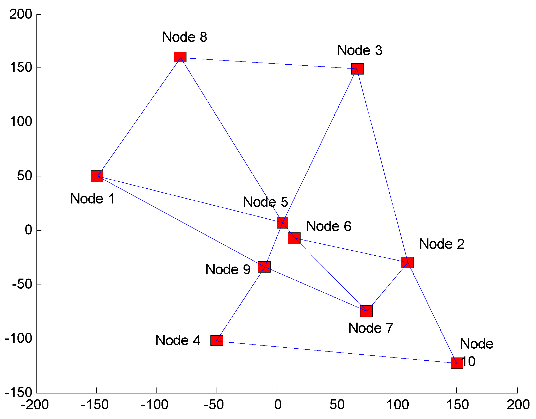
We tested the performance of the proposed algorithm by conducting simulations involving graphs with various numbers of nodes, i.e., 10, 15, and 20 nodes, as shown in Figure 3, Figure 4 and Figure 5, respectively. For each graph, four variations of connectivity were simulated to show the success of finding solutions. We denoted the graph, together with the connectivity of variations, by using the code “CONFIG A-B”, where A is the number of nodes and B is the label of a variation. For instance, the first variation of the graphs with 10, 15, and 20 nodes were denoted as CONFIG 10-1, CONFIG 15-1, and CONFIG 20-1, respectively. Note that all edges were bi-directional.

Three significant aspects were evaluated. The first aspect was the influence of minimum allowable arrival time on the solution’s existence and the convergence of the solutions. The second was the correlation between the average degrees of all nodes, the number of vehicles, and the number of nodes to the success of finding solutions. The last aspect was the accuracy of the resulted minimum traveling time of the slowest vehicle, according to the variation of the evaporating constant and its effect on the convergence of the search results.

For evaluating the first and third aspects, we established simulations for three vehicles, where the 1st, 2nd, and 3rd vehicles started from Nodes 4, 1, and 3, respectively. Each vehicle had four speed options, i.e., 0.1, 0.5, 1, and 1.5 m/s. Meanwhile, for evaluating the second aspect, we applied two until seven vehicles on each connectivity configuration. Vehicles 1 until 7 were started from Nodes 4, 1, 3, 5, 10, 7, and 8, respectively. For one simulation, we applied 3000 iterations of searching the optimal solution.

5.1. The Effect of Minimum Allowable Arrival Time Difference $t_{occ}$

The first simulation set was established to evaluate the relation between the minimum allowable arrival time difference, $t_{\mathrm{occ}}$, and the solution’s existence. The purpose of the simulations is to confirm the hypotheses. In such simulations, we used $\alpha =1$ and $\beta =1$ and evaporate rate $\rho =0.95$. We applied five values of $t_{occ}$, i.e., 10, 50, 100, 150, and 300 s.

Table 1. Simulation results for various $t_{\mathrm{occ}}$ for three vehicles.

(1)	(2)	(3)	(4)	(5)
$t_{\mathrm{occ}}$(s)	$n_{\mathrm{success}}$	$T_{\mathrm{avg}}$(s)	${\sigma }_{\mathrm{T}}$(s)	$T_{\min }$(s)
10.00	10	1754.16	320.69	1482.50
50.00	9	2648.04	663.91	1896.30
100.00	8	3412.84	1191.16	1961.10
150.00	8	3314.01	841.83	1684.20
300.00	5	3735.32	1180.45	2851.00

and

Table 2. Simulation results for various evaporate constants at $t_{\mathrm{occ}}>150$ s.

(1)	(2)	(3)	(4)	(5)
$\rho$	$n_{\mathrm{success}}$	$T_{\mathrm{avg}}$(s)	${\sigma }_{\mathrm{T}}$(s)	$T_{\min }$
0.1	9	2977.72	732.50	1949.00
0.2	7	3317.33	636.00	2189.30
0.3	6	2269.77	403.38	1744.00
0.4	8	3213.81	777.59	1966.40
0.5	9	2929.99	609.94	2064.70

show the results of 10 trials for varying allowable minimum occupation time $t_{\mathrm{occ}}$ and varying evaporate constant $\rho$, respectively. In each table, as shown in Column (1), for each occupation time, we established five trials. Column (1) reveals the values of ${\mathrm{t}}_{\mathrm{occ}}$. Column (2) is the success rate of finding a complete solution. Columns (3) and (4) show the average and standard deviation of the maximum traveling times, respectively. Column (5) shows the minimum value of maximal traveling times.

The application of $t_{\mathrm{occ}}$ is evaluated for its effect on the percentage of successful trials from 10 trials, i.e., $n_{\mathrm{success}}$, average traveling time of the slowest vehicle, $T_{\mathrm{avg}}$, the standard deviation of $T_{\mathrm{avg}}$, i.e., ${\sigma }_{\mathrm{T}}$, and the minimum traveling time that is ever found from the ten trials, i.e., $T_{\min }$. For this purpose, we use a statistical correlation technique. The correlations between $t_{\mathrm{occ}}$ and $n_{\mathrm{success}}$, $T_{\mathrm{avg}}$, ${\sigma }_{\mathrm{T}}$, and $T_{\min }$ are −0.99, 0.83, 0.75, and 0.88, respectively. In can be concluded that there is a strong negative relationship between $t_{\mathrm{occ}}$, = and $n_{\mathrm{success}}$ and almost-strong positive relation between $t_{\mathrm{occ}}$ and the other three variables. In addition, the tendency of failure can be identified by a parameter ${\sigma }_{\mathrm{T}}/{\mathrm{t}}_{\mathrm{occ}}$. We found from the simulation that ${\sigma }_{\mathrm{T}}/{\mathrm{t}}_{\mathrm{occ}}$ is directly proportional to the probability of success in finding a solution, i.e., $n_{\mathrm{success}}$.

5.2. Successfulness of Finding a Solution

Since the graph is not fully connected, it is possible that there exists a situation such that any single solution is failed to find as the effect of the number of nodes, the average degree of all nodes increase, and the number of vehicles. The degree of a node is defined as the number of edges that connect to the node. We established simulations for 10, 15, and 20 nodes under $t_{\mathrm{occ}}=10 \mathrm{s}$.

5.2.1. Simulations for 10 Nodes

For the ten nodes cases, we applied four different configurations of connectivity, as shown in

Table 3. Simulation results for 10 nodes.

	Number of Degree of Nodes
Node	CONFIG 10-1		CONFIG 10-2		CONFIG 10-3		CONFIG 10-4
1	3		3		3		4
2	4		4		4		4
3	3		3		3		4
4	2		2		2		4
5	5		4		3		5
6	3		3		3		4
7	3		3		3		5
8	3		2		2		3
9	4		4		3		4
10	2		2		2		3
Average	3.20		3.00		2.80		4.00
Number of Vehicles	φ	Success Rate (%)	φ	Success Rate (%)	φ	Success Rate (%)	φ	Success Rate (%)
3	0.09	100.00	0.10	100.00	0.11	100.00	0.08	100.00
4	0.13	90.00	0.13	100.00	0.14	100.00	0.10	100.00
5	0.16	100.00	0.17	100.00	0.18	100.00	0.13	100.00
6	0.19	90.00	0.20	90.00	0.21	0.00	0.15	100.00
7	0.22	0.00	0.23	0.00	0.25	0.00	0.18	90.00

, i.e., CONFIGs 10-1, 10-2, 10-3, and 10-4. CONFIG 10-1 is the graph with the connectivity visualized in Figure 3. CONFIG 10-2 is constructed from CONFIG 10-1 with the elimination of the edge connecting Nodes 5 to 8. CONFIG 10-3 is constructed from CONFIG 10-3, with the elimination of the edge connecting Nodes 5 to 9. CONFIG 10-4 is constructed from the CONFIG 10-1, with the addition of the edges connecting Nodes 1 to 4, 3 to 6, and 4 to 7. Table 3 describes the degree of each node. The averages of the degree of nodes for CONFIG 10-1, 10-2, 10-3, and 10-4 are 3.20, 3.00, 2.80, and 4.00.

We investigate the relationship between the nodes’ average degrees and the number of vehicles to the possibility of successfulness of finding a solution. Here, we introduce a parameter $\varphi$ defined as follows:

$$\varphi =\frac{N_{\mathrm{u}}}{r_{\mathrm{avg} }{N}_{\mathrm{v}}},$$

(12)

where $r_{\mathrm{avg} }$ is defined as the average degree of all nodes. From Table 3, it can be seen that the solution can be found for $\varphi \le 0.19$. It can be concluded that, from the 10 trials, at the range of the $\varphi$, there exists at least one successful trial.

5.2.2. Simulations for 15 Nodes

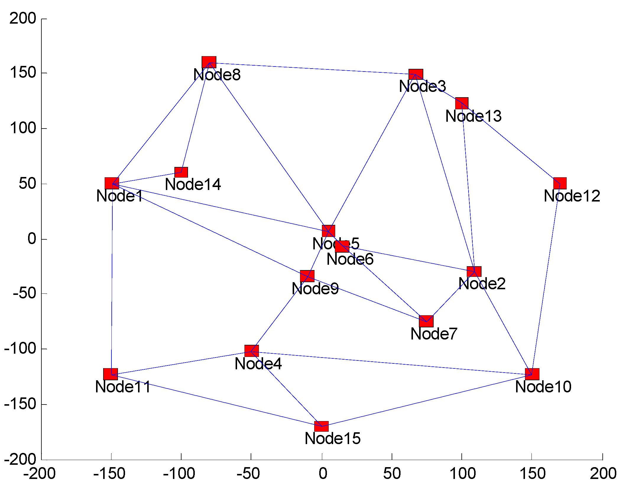
In this simulation, we added five nodes, as follows. Nodes 11, 12, 13, 14, and 15 are located at (−150 m, −123 m), (170 m, 50 m), (100 m, 123 m), (−100 m, 60 m), and (0 m, −170 m), respectively. Moreover, four edges configurations in the new graph were established, called CONFIG 15-1, CONFIG 15-2, CONFIG 15-3, and CONFIG 15-4. The CONFIG 15-1 connectivity configuration is described in Figure 4. CONFIG 15-2 is constructed by adding an edge connecting Nodes 1 and 5 on the CONFIG 15-1. The CONFIG 15-3 configuration is performed by adding edges connecting Nodes 1 to 4, 2 to 12, and 7 to 10 to CONFIG 15-2. The CONFIG 15-4 configuration is performed by adding edges connecting nodes 4 to 7 and 3 to 6 to CONFIG 15-3. The degree of each edge in each connectivity configuration is described in

Table 4. Simulation results for 15 nodes.

	Number of Degree of Nodes
Node	CONFIG 15-1		CONFIG 15-2		CONFIG 15-3		CONFIG 15-4
1	5		5		6		6
2	5		5		6		6
3	4		4		4		5
4	4		4		5		6
5	5		6		6		6
6	3		3		3		4
7	3		3		4		5
8	4		4		4		4
9	4		4		4		4
10	4		4		5		5
11	3		3		3		3
12	2		2		3		3
13	3		3		3		3
14	2		3		3		3
15	3		3		3		3
Average	3.60		3.73		4.13		4.40
Number of Vehicles	φ	Success Rate (%)	φ	Success Rate (%)	φ	Success Rate (%)	φ	Success Rate (%)
3	0.06	100.00	0.05	100.00	0.05	90.00	0.05	90.00
4	0.07	90.00	0.07	90.00	0.06	90.00	0.06	100.00
5	0.09	10.00	0.09	20.00	0.08	10.00	0.08	50.00
6	0.11	0.00	0.11	0.00	0.10	0.00	0.09	0.00
7	0.13	0.00	0.13	0.00	0.11	0.00	0.11	0.00

.

From Table 4, it can be seen that the solution can be found for $\varphi \le 0.08$, which means that, at the range of the $\varphi$, it can be concluded that, from the 10 trials, there always exists at least one successful trial.

5.2.3. Simulations for 20 Nodes

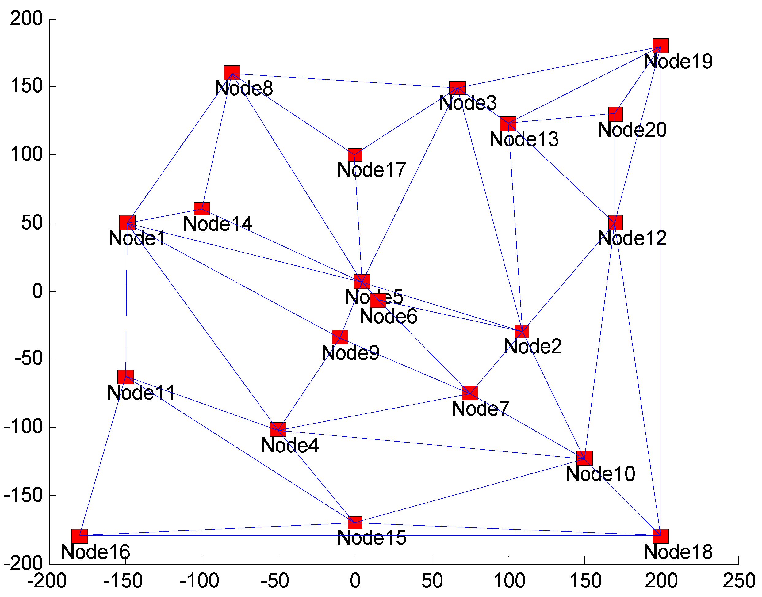
In this simulation, we added five nodes from the CONFIG 15-1, as follows. Nodes 16, 17, 18, 19, and 20 are located at (−100 m, −180 m), (0 m, 100 m), (200 m, −180 m), (200 m, 180 m), and (170 m, 130 m), respectively. Similar to the simulation for 15 nodes, we define four edge configurations in the new graph, namely CONFIG 20-1, CONFIG 20-2, CONFIG 20-3, and CONFIG 20-4. The CONFIG 20-1 connectivity configuration is described in Figure 5. CONFIG 20-2 is constructed by modifying CONFIG 20-1, i.e., adding edges connecting Nodes 1 to 16, 4 to 16, 2 to 20, 6 to 9, 8 to 19, and 12 to 17. CONFIG 20-3 is performed by adding Edges 2 to 17, 3 to 5 to 9, 7 to 15, and 9 to 15 and eliminating Edges 4 to 16, 4 to 10, and 14 to 17 on CONFIG 20-2. CONFIG 20-4 is performed by the addition of Edges 3 to 17, 4 to 16, 4 to 10, and 5 to 14 to CONFIG 20-3.

Table 5. Simulation results for 20 nodes.

	Number of Degree of Nodes
Node	CONFIG 20-1		CONFIG 20-2		CONFIG 20-3		CONFIG 20-4
1	6		7		7		7
2	7		8		9		9
3	6		6		6		7
4	6		7		5		7
5	8		8		9		10
6	3		4		4		4
7	5		4		5		5
8	5		5		5		5
9	4		5		6		6
10	6		6		5		6
11	4		4		4		4
12	6		7		8		8
13	5		5		6		6
14	3		4		4		5
15	5		5		7		7
16	3		5		4		5
17	3		4		5		6
18	5		5		5		5
19	5		6		6		6
20	3		4		5		5
Average	4.90		5.45		5.75		6.15
Number of Vehicles	φ	Success Rate (%)	φ	Success Rate (%)	φ	Success Rate (%)	φ	Success Rate (%)
2	0.02	10.00	0.02	100.00	0.02	100.00	0.02	100.00
3	0.03	0.00	0.03	90.00	0.03	100.00	0.02	90.00
4	0.04	0.00	0.04	0.00	0.03	80.00	0.03	90.00
5	0.05	0.00	0.05	0.00	0.04	0.00	0.04	0.00
6	0.06	0.00	0.06	0.00	0.05	0.00	0.05	0.00
7	0.07	0.00	0.06	0.00	0.06	0.00	0.06	0.00

reveals the simulation results of such connectivity configurations. It can be shown that the solution can be found for $\varphi \le 0.02$. It means that, from the 10 trials, it can be concluded that there always exists at least one successful trial at the range of the $\varphi$.

5.3. Analysis of Accuracy

From the simulations established in Section 5.3, we can analyze the accuracy of the result, i.e., minimum traveling time of the slowest vehicle. The standard deviation ${\sigma }_{\mathrm{T}}$ can identify the accuracy of the simulation. As shown in Table 1 and Table 2, the averages of ${\sigma }_{\mathrm{T}}$ for ${\mathrm{t}}_{\mathrm{occ}}>10$ s and ${\mathrm{t}}_{\mathrm{occ}}>150$ s are 373.48 s and 631.2 s. It indicates that the results in lower $t_{\mathrm{occ}}$ are more accurate than the higher ones.

In addition, we analyzed the relationship between the average $T_{\mathrm{avg}}$ and ${\sigma }_{\mathrm{T}}$ by using the same technique as the one used in Section 5.2., i.e., statistical correlation. The results are described as follows. The correlations between $T_{\mathrm{avg}}$ and ${\sigma }_{\mathrm{T}}$ for ${\mathrm{t}}_{\mathrm{occ}}>10$ s and ${\mathrm{t}}_{\mathrm{occ}}>150$ s are 0.92 and 0.84, respectively. It indicates that there is a relatively strong positive relation between $T_{\mathrm{avg}}$ and ${\sigma }_{\mathrm{T}}$: larger $T_{\mathrm{avg}}$ tends to lead to a larger ${\sigma }_{\mathrm{T}}$, or, in other words, a larger $T_{\mathrm{avg}}$ tends to lead to lower accuracy.

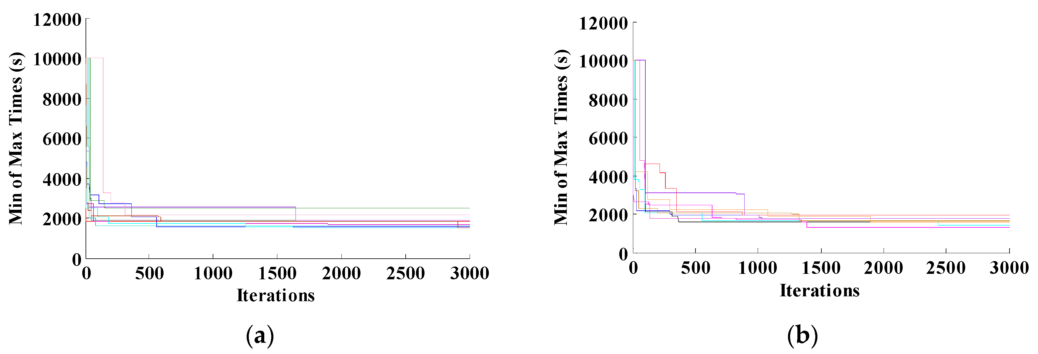
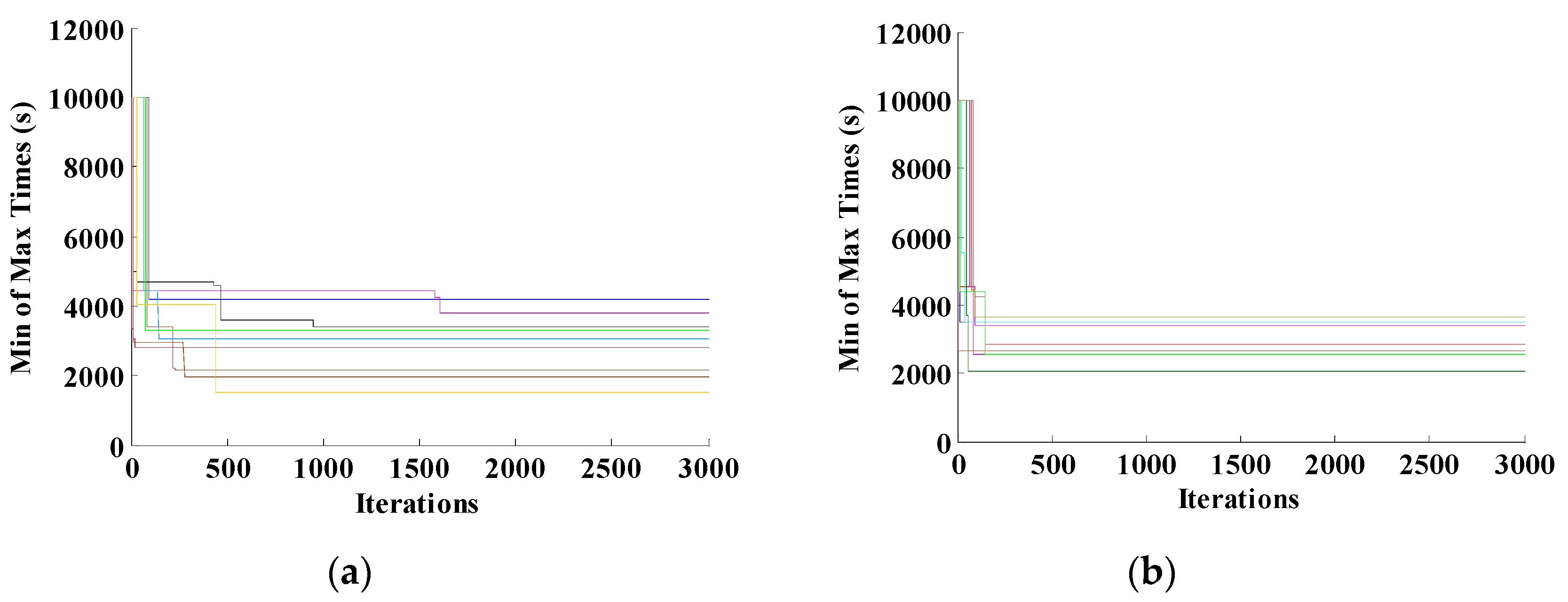
Figure 6 and Figure 7 show the searching progression for ${\mathrm{t}}_{\mathrm{occ}}>10$ s and ${\mathrm{t}}_{\mathrm{occ}}>150$ s, respectively, each with $\rho =0.1$ and $\rho =0.5$. It can be concluded that the algorithm’s ability to converge is better for ${\mathrm{t}}_{\mathrm{occ}}>10$ s than for ${\mathrm{t}}_{\mathrm{occ}}>150$ s. It can be concluded from the final values until the 3000th iteration. Moreover, Figure 6 and Figure 7 confirm the accuracy conclusions conducted from the statistical correlation analysis. Accuracy analysis can infer other behavior, that is, the ability to reach $T_{\mathrm{avg}}$. Figure 7 shows that, for ${\mathrm{t}}_{\mathrm{occ}}>10$ s, the algorithm’s ability to reach $T_{\mathrm{avg}}$ is better than that for $t_{\mathrm{occ}}>150$ s. Furthermore, it can be seen that, for $t_{\mathrm{occ}}>150$ s, even until the 1500th iteration, the algorithm still can update the minimum of maximum times. However, it cannot go further to $T_{\mathrm{avg}}$. The interesting situation occurs for $\rho =0.5$ in the same $t_{\mathrm{occ}}$. In this situation, mostly, once a solution is found, the algorithm cannot find another better solution.

5.4. The Near-Optimal Trajectories

We show two samples of near-optimal trajectories obtained from the simulations to verify that any point in the graph G is visited by different vehicles with the arrival time difference between any vehicles exceeds ${\mathrm{t}}_{\mathrm{occ}}$.

Table 6. Most near-optimal trajectories for ${\mathrm{t}}_{\mathrm{occ}}>10$ s.

Vehicle 1	Routes	4	10	2	6	7	9	1	5	3	8
	Arrival Time (s)	0	365.6	446.9	511.5	584.0	659.5	767.8	874.4	998.3	1194.9
	Applied Speed (m/s)	0.1	1	1.5	1.5	1	1.5	1.5	1.5	1	1.5
Vehicle 2	Routes	1	5	6	7	9	4	10	2	3	8
	Arrival Time (s)	0	290.7	313.6	404.3	467.3	565.9	817.2	944.3	1174.1	1292.0
	Applied Speed (m/s)	1	1	0.5	1.5	1.5	0.1	1.5	0.1	1.5	1
Vehicle 3	Routes	3	8	5	1	9	7	6	2	10	4
	Arrival Time (s)	0	184.3	403.0	602.9	711.2	786.7	859.2	956.0	1091.5	1292.6
	Applied Speed (m/s)	0.1	1.5	0.1	1.5	1.5	1	1.5	0.5	1	1

and

Table 7. Most near-optimal trajectories for ${\mathrm{t}}_{\mathrm{occ}}>150$ s.

Vehicle 1	Routes	4	10	2	6	5	3	8	1	9	7
	Arrival Time (s)	0	670.3	805.8	981.8	1003.3	1106.6	1290.9	1723.7	1886.1	1949.0
	Applied Speed (m/s)	0.1	0.5	1	0.1	1.5	1.5	0.1	0.5	1.5	1.5
Vehicle 2	Routes	1	8	5	3	2	10	4	9	7	6
	Arrival Time (s)	0	432.8	666.2	872.8	1240.5	1342.2	1476.2	1539.3	1710.9	1875.8
	Applied Speed (m/s)	0.1	0.5	1	0.5	0.5	1.5	1.5	1	0.1	1
Vehicle 3	Routes	3	8	5	1	9	4	10	2	6	7
	Arrival Time (s)	0	184.3	324.3	537.5	754.0	832.9	993.8	1075.1	1171.9	1262.6
	Applied Speed (m/s)	0.1	1.5	1	0.5	1	1	1.5	1	1	1

show the optimal trajectories for $t_{\mathrm{occ}}>10$ s and $t_{\mathrm{occ}}>150$ s, respectively. To verify that the arrival time differences exceed $t_{\mathrm{occ}}$, we provide

Table 8. Arrival time difference for ${\mathrm{t}}_{\mathrm{occ}}>10$ s and ${\mathrm{t}}_{\mathrm{occ}}>150$ s.

	$\mathbf{For} {\mathit{t}}_{\mathit{o}\mathit{c}\mathit{c}}>10 \mathbf{s}$			$\mathbf{For}{\mathit{t}}_{\mathit{o}\mathit{c}\mathit{c}}>150 \mathbf{s}$
Nodes	Vehicles 1 and 2	Vehicles 1 and 3	Vehicles 2 and 3	Vehicles 1 and 2	Vehicles 1 and 3	Vehicles 2 and 3
1	767.8	364.8	403	1723.7	1186.2	537.5
2	497.4	509.1	11.7	434.7	269.3	165.4
3	175.8	998.3	1174.1	233.8	1106.6	872.8
4	565.9	1292.6	726.7	1476.2	832.9	643.3
5	583.7	471.4	112.3	337.1	679	341.9
6	197.9	347.7	545.6	894	190.1	703.9
7	179.7	202.7	382.4	238.1	686.4	448.3
8	97.1	1010.6	1107.7	858.1	1106.6	248.5
9	192.2	51.7	243.9	346.8	1132.1	785.3
10	451.6	725.9	274.3	671.9	323.5	348.4

. According to Table 8, for $t_{\mathrm{occ}}>10$ s, the smallest arrival time difference is 11.7 s, i.e., between Vehicles 2 and 3 at Node 2. For $t_{\mathrm{occ}}>150$ s, the smallest arrival time difference is 165.4 s, i.e., between Vehicles 2 and 3 at Node 2.

6. Conclusions

A method to solve the Collision-Free Multiple Traveling Salesman Problem (CFMTSP) applied to multiple agents was proposed. In this problem, each agent must visit all nodes in a provided graph, following the provided edges. The graph is modified into an augmented graph such that the information of nodes’ position and speed options can be accommodated, and in turn, the arrival time to each node can be determined. According to the optimization of collision-free for each vehicle, an ACO involving multiple ant species is utilized on the augmented graph. The pheromone trails are not left on the edges (such as in typical graph model), but the augmented edges. As a consequence, the probability of selection is assigned to those augmented edges, as well. As a result, the solution is not the sequence of routes but also the trajectory (routes and selected speeds). The algorithm has to guarantee that the resulted trajectories are collision-free.

Simulations were established with no violation of minimum allowable arrival time difference. In addition, the simulations have shown three behaviors of the resulted solutions. First, the increase of minimum allowable arrival time difference leads to the decrease of the number of successful trials, almost-strongly increases of the average, the standard deviation, and the ever-found minimum traveling times. Second, it can be concluded that there exists a threshold of the ratio $\varphi$ such that the solution for all vehicles is unable to find. It was demonstrated that the threshold of $\varphi$ is lower as the number of nodes increases. Moreover, for the same number of nodes, the increase of the average of nodes’ degree leads to the number of vehicles that are able to find solutions successfully. Third, it is concluded that that the increase in the average of minimum traveling time tends to decrease the algorithm’s accuracy. Third, the evaporate rate in the algorithm has a weak influence on the average, the standard deviation, and the ever-found minimum traveling times.

Future works will focus on some issues, such as the continuation of speed options and the consequences of modifying the augmented graph. Another issue is in the performance of the ACO algorithm, such as the convergence of the optimal trajectories, the decrease of the standard deviation of the slowest agent’s traveling time in high minimum allowable arrival time difference.

References

- Li, Y.; Soleimani, H.; Zohal, M. An improved ant colony optimization algorithm for the multi-depot green vehicle routing problem with multiple objectives. J. Clean. Prod. 2019, 227, 1161–1172. [Google Scholar] [CrossRef]
- Bae, H.; Moon, I. Multi-depot vehicle routing problem with time windows considering delivery and installation vehicles. Appl. Math. Model 2016, 40, 13–14. [Google Scholar] [CrossRef]
- Mandziuk, J.; Swiechowski, M. UCT in capacitated vehicle routing problem with traffic jams. Inf. Sci. 2017, 406–407, 42–56. [Google Scholar] [CrossRef]
- Bektas, T. The multiple traveling salesman problem: An overview of formulations and solution procedures. Omega 2006, 34, 209–219. [Google Scholar] [CrossRef]
- Lawler, E.L. The Travelling Salesman Problem: A Guided Tour of Combinatorial Optimization; John Wiley and Sons: Hoboken, NJ, USA, 1985. [Google Scholar]
- Golden, B.; Raghavan, S.; Wasil, E.A. The vehicle routing problem: Latest advances and new challenges, operations research. In Computer Science Interfaces Series; Springer: Berlin/Heidelberg, Germany, 2008; Volume 43. [Google Scholar]
- Khachay, M.; Neznakhina, K. Polynomial time solvable subclass of the generalized traveling salesman problem on grid clusters. In Proceedings of the International Conference on Analysis of Images, Social Networks and Texts, Moskow, Russia, 5–7 July 2017; pp. 346–355. [Google Scholar]
- Chalarux, T.; Sripratak, P. Worst case analyses of nearest neighbor heuristic for finding the minimum weight K-cycle. Curr. Appl. Sci. Technol. 2020, 20, 178–185. [Google Scholar]
- Khachay, M.; Neznakhina, K. Approximability of the minimum-weight k-size cycle cover problem. J. Glob. Optim. 2016, 66, 65–82. [Google Scholar] [CrossRef]
- Fazlollahtabar, H.; Saidi-Mehrabad, M. Mathematical model for deadlock resolution in multiple AGV scheduling and routing network: A case study. Ind. Robot. 2015, 42, 252–263. [Google Scholar] [CrossRef]
- Vivaldini, K.; Rocha, L.F.; Martarelli, N.J.; Becker, M.; Moreira, A.P. Integrated tasks assignment and routing for the estimation of the optimal number of AGVS. Int. J. Adv. Manuf. Technol. 2016, 82, 719–736. [Google Scholar] [CrossRef]
- Hu, W.; Mao, J.; Wei, K. Energy-efficient rail guided vehicle routing for two-sided loading/unloading automated freight handling systems. Eur. J. Oper. Res. 2017, 258, 943–957. [Google Scholar] [CrossRef] [Green Version]
- Adamo, T.; Bektas, T.; Ghiani, G.; Guerriero, E.; Manni, E. Path and speed optimization for conflict-free pickup and delivery under time windows. Trans. Sci. 2018, 52, 739–755. [Google Scholar] [CrossRef] [Green Version]
- Zhong, M.; Yang, Y.; Dessouky, Y.; Postolache, O. Multi-AGV scheduling for conflict-free path planning in automated container terminals. Comput. Ind. Eng. 2020, 142, 106371. [Google Scholar] [CrossRef]
- Ali, I.M.; Essam, D.; Kasmarik, K. A novel design of differential evolution for solving discrete traveling salesman problems. Swarm Evol. Comput. 2020, 53, 100607. [Google Scholar] [CrossRef]
- Baniasadi, P.; Foumani, M.; Smith-Miles, K.; Ejov, V. A transformation technique for the clustered generalized traveling salesman problem with application to logistics. Eur. J. Oper. Res. 2020, 2, 444–457. [Google Scholar] [CrossRef]
- Pacheco-Valencia, V.; Hernandez, J.A.; Sigaretta, J.M.; Vakhania, N. Simple constructive, insertion, and improvement heuristics based on the girding polygon for the Euclidean traveling salesman problem. Algorithms 2020, 13, 5. [Google Scholar] [CrossRef] [Green Version]
- Pandiri, V.; Singh, A. An artificial bee colony algorithm with variable degree of perturbation for the generalized covering traveling salesman. Appl. Soft Comput. 2019, 78, 481–495. [Google Scholar] [CrossRef]
- Held, M.; Karp, R.M. The traveling salesman problem and minimum spanning tree. Oper. Res. 1970, 18, 1138–1162. [Google Scholar] [CrossRef]
- Fiechter, C.-N. A parallel tabu search algorithm for large traveling salesman problem. Discret. Appl. Math. 1994, 51, 243–267. [Google Scholar] [CrossRef] [Green Version]
- Siqueira, P.H.; Steiner, M.T.A.; Scheer, S. A new approach to solve the traveling salesman problem. Neurocomputing 2007, 70, 1013–1021. [Google Scholar] [CrossRef]
- Rego, C.; Gamboa, D.; Glover, F.; Osterman, C. Traveling salesman problem heuristics: Leading methods, implementations and latest advances. Eur. J. Oper. Res. 2011, 211, 427–441. [Google Scholar] [CrossRef]
- Essani, F.H.; Haider, S. An algorithm for mapping the asymmetric multiple traveling salesman problem onto colored petri nets. Algorithms 2018, 11, 143. [Google Scholar] [CrossRef] [Green Version]
- Groba, C.; Sartal, A.; Vasquez, X.H. Integrating forecasting in metaheuristic methods to solve dynamic routing problems: Evidence from the logistic processes of tuna vessels. Eng. Appl. Artif. Intel. 2018, 76, 55–66. [Google Scholar] [CrossRef]
- Xu, W.; Guo, S.; Li, X.; Guo, C.; Wu, R.; Peng, Z. A dynamic scheduling method for logistics tasks oriented to intelligent manufacturing workshop. Math. Probl. Eng. 2019, 2019, 7237459. [Google Scholar] [CrossRef]
- Pandiri, V.; Singh, A. A swarm intelligence approach for the colored traveling salesman problem. Appl. Intell. 2018, 48, 4412–4428. [Google Scholar] [CrossRef]
- Lu, L.-C.; Yue, T.-W. Mission-oriented ant-team ACO for min–max MTSP. Appl. Soft. Comput. 2019, 76, 436–444. [Google Scholar] [CrossRef]
- Dorigo, M.; Gambardella, L. Ant colony: A cooperative learning approach to the travelling salesman problem. IEEE Trans. Evol. Comput. 1997, 1, 53–66. [Google Scholar] [CrossRef] [Green Version]
- Widyotriatmo, A.; Hong, K.-S. Navigation function-based control of multiple wheeled vehicles. IEEE Trans. Ind. Electron. 2011, 58, 1896–1906. [Google Scholar] [CrossRef]
- Fraichard, T.; Asama, H. Inevitable collision states—A step towards safer robots? Adv. Robot. 2004, 18, 1001–1024. [Google Scholar] [CrossRef] [Green Version]
- Snape, J.; van den Berg, J.; Guy, S.J.; Manocha, D. The hybrid reciprocal velocity obstacle. IEEE Trans. Robot. 2011, 27, 696–706. [Google Scholar] [CrossRef] [Green Version]
- Alonso-Mora, J.; Beardsley, P.; Siegwart, R. Cooperative collision avoidance for nonholonomic robots. IEEE Trans. Robot. 2018, 34, 404–420. [Google Scholar] [CrossRef] [Green Version]
- Makarem, L.; Gillet, D. Model predictive coordination of autonomous vehicles crossing intersections. In Proceedings of the 16th International IEEE Conference on Intelligent Transportation Systems (ITSC), Hague, The Netherlands, 6–9 October 2013. [Google Scholar]
- Mahbub, A.M.I.; Malikopoulos, A.A.; Zhao, L. Decentralized optimal coordination of connected and automated vehicles for multiple traffic scenarios. Automatica 2020, 117, 108958. [Google Scholar] [CrossRef] [Green Version]
- Tan, C.Y.; Huang, S.; Tan, K.K.; Teo, R.S.H. Three-dimensional collision avoidance for multi unmanned aerial. Vehicles Using Velocity Obstacle. J. Intell. Robot. Syst. 2020, 97, 227–248. [Google Scholar] [CrossRef]
- Pamosoaji, A.K.; Piao, M.; Hong, K.-S. PSO-based minimum-time motion planning for multiple-vehicle systems considering acceleration and velocity limitations. Int. J. Control Autom. Syst. 2019, 17, 2610–2623. [Google Scholar] [CrossRef]
- Yu, M.; Qi, X. A Vehicle routing problem with multiple overlapped batches. Trans. Res. E 2014, 61, 40–55. [Google Scholar] [CrossRef]
- Baranwal, M.; Roehl, B.; Salapaka, S.M. Multiple traveling salesmen and related problems: A maximum-entropy principle-based approach. In Proceedings of the 2017 American Control Conference (ACC), Seattle, WA, USA, 24–26 May 2017. [Google Scholar]
- Pamosoaji, A.K.; Hong, K.-S. Group-based particle swarm optimization for multiple-vehicles trajectory planning. In Proceedings of the 15th International Conference on Control, Automation, and Systems (ICCAS), Busan, Korea, 13–16 October 2015; pp. 862–867. [Google Scholar]
- Chalissery, J.M.; Renyard, A.; Gries, R.; Hoefele, D.; Alamsetti, S.K.; Gries, G. Ant sense, and follow, trail pheromones of ant community members. Insects 2019, 10, 383. [Google Scholar] [CrossRef] [Green Version]
Figure 1.
Augmented nodes and edges.
Figure 2.
The proposed augmented graph.
Figure 3.
Graph with CONFIG 10-1 configuration (10 nodes).
Figure 4.
Graph with CONFIG 15-1 configuration (15 nodes).
Figure 5.
Graph with CONFIG 20-1 configuration (20 nodes).
Figure 6.
The progression of searching the optimal solution for s: (a) for ; (b) .
Figure 7.