Generalized Polynomial Chaos Expansion for Fast and Accurate Uncertainty Quantification in Geomechanical Modelling

Abstract

Geomechanical modelling of the processes associated to the exploitation of subsurface resources, such as land subsidence or triggered/induced seismicity, is a common practice of major interest. The prediction reliability depends on different sources of uncertainty, such as the parameterization of the constitutive model characterizing the deep rock behaviour. In this study, we focus on a Sobol’-based sensitivity analysis and uncertainty reduction via assimilation of land deformations. A synthetic test case application on a deep hydrocarbon reservoir is considered, where land settlements are predicted with the aid of a 3-D Finite Element (FE) model. Data assimilation is performed via the Ensemble Smoother (ES) technique and its variation in the form of Multiple Data Assimilation (ES-MDA). However, the ES convergence is guaranteed with a large number of Monte Carlo (MC) simulations, that may be computationally infeasible in large scale and complex systems. For this reason, a surrogate model based on the generalized Polynomial Chaos Expansion (gPCE) is proposed as an approximation of the forward problem. This approach allows to efficiently compute the Sobol’ indices for the sensitivity analysis and greatly reduce the computational cost of the original ES and MDA formulations, also enhancing the accuracy of the overall prediction process.

1. Introduction

Geomechanical modelling is a scientific and engineering activity of paramount importance to evaluate the safety and predict possible environmental impacts related to the exploitation of subsurface resources. The reliability of the predictions depends on different sources of uncertainty, which are somewhat intrinsically introduced in any modelling process. Uncertainty typically affects the knowledge of the constitutive rock behaviour, the geometry of the depleted formations, the diffusion of the pressure perturbation, just to mention a few important occurrences. In this study, we focus on the reduction of uncertainty affecting the constitutive model parameters and the land subsidence prediction via assimilation of ground surface displacements.

A synthetic test case application dealing with the depletion of a deep hydrocarbon reservoir is considered. Land settlements are predicted with the aid of a 3-D Finite Element (FE) model using a one-way coupled approach [1,2,3]. The focus is on the calibration of the rock constitutive parameters that mainly control the compaction of the rock formation caused by the hydrocarbon production. Assuming the use of some well-established constitutive models, such as Mohr-Coulomb, Modified Cam-Clay, hypo-elastic, hypo-plastic or visco-elasto-plastic laws [4,5,6,7], different approaches can be used to estimate the governing parameters. If the required parameters have a measurable physical meaning, a major investigation branch concerns either laboratory tests, properly developed for characterization of geological formations [8], or in-situ observations employed to study reservoir deformation with specific measurement apparatus, for example, well-logs equipped with radioactive markers [9]. Another important approach, which is especially related to those parameters that are not directly associated to measurable quantities, deals with inverse models to infer the uncertain model parameters using either deterministic or stochastic techniques. The latter approaches are increasingly employed in geomechanics. For example, in References [10,11] the Ensemble Smoother (ES), that is, a Monte Carlo (MC)-based method, is used to estimate the parameters of a transversely isotropic and isotropic constitutive law by the joint assimilation of horizontal and vertical displacements. Later developments of the ES algorithm in the form of Multiple Data Assimilation (ES-MDA) are used in Reference [12] to constrain the reservoir compaction coefficient and the subsurface basement elastic modulus by assimilation of ascending and descending line-of-sight displacements revealed by Permanent Scatterer Interferometry (PSI). Recently, Reference [13] compares the results obtained from applying the ES and the ES-MDA to estimate the parameters of the modified Cam-Clay and the Vermeer-Neher (VN) visco-elasto-plastic models [3].

The growing interest on the ES as a data assimilation technique is mainly due to its straightforward implementation and the capability of using simultaneously the measurements collected at different times and locations in a 4-D assimilation. However, its convergence is guaranteed only with a large number of MC simulations that may be computationally unfeasible in demanding large-scale problems. Moreover, its effectiveness in constraining the model for a strongly non-linear dependence of the outcome on the uncertain parameters is theoretically questionable. This limitation can be overcome by employing the ES in a multiple assimilation fashion, with the introduction of the ES-MDA technique [14], but this implies a further significant increase of the computational cost for the overall procedure, with the ES algorithm repeatedly applied to different ensembles. It follows the need for fast model predictions that can be achieved by approximating the forward model operators with surrogate solutions, obtained at a highly reduced computational cost.

In geomechanical applications, surrogate models have been recently employed for uncertainty quantification (UQ) and sensitivity analysis (SA). A functional data analysis technique is used to perform a vertical displacements UQ on a synthetic field-scale test by setting the oedometric compressibility as uncertain parameter [15]. Polynomial chaos proxies of the linear poroelastic problem with hydromechanical coupling allows a variance-based SA on Lamé’s constants, the Biot-Willis coefficient and the hydraulic mobility [16]. Another non-intrusive approach is used in sequentially coupled reservoir-geomechanical simulations to estimate the caprock safety factor in a probabilistic setting [17]. Global SA and parameter identification are carried out by means of Gaussian processes in a carbon capture and storage test case to model fault poromechanics and induced seismicity in a stochastic framework [18]. A similar approach is used in Reference [19] to investigate the onset of fault activation in deep hydrocarbon reservoirs with surrogates based on polynomial chaos expansion. Global SA are also employed to investigate geomechanical fractured reservoirs [20] and hydraulically fractured wells with reduced order models [21].

In this work, we focus our attention on the generalized polynomial chaos expansion (gPCE) [22,23,24,25,26]. Using a spectral representation in the random space, gPCE-stochastic solutions are expressed by orthogonal polynomials of the input parameters [27]. This approach has already proved successful in several different engineering applications [28,29] with a growing interest in the Earth science community for UQ and SA [30,31,32,33,34,35]. Moreover, gPCE is suitable for identification problems in the Bayesian inference framework as documented in previous studies [36,37,38,39,40], to cite just a few.

Here we present an approach where we further extend the use of the gPCE as surrogate for regional geomechanical models with the aim of land subsidence prediction due to the exploitation of subsurface resources. Our contribution is threefold: (i) to validate the gPCE surrogate model for a highly non-linear consitutive law such as the VN visco-elasto-plastic model, (ii) to perform a global SA and rank the influence of the model parameters and their combinations, and (iii) based on sensitivity results, to adapt accordingly the probabilistic framework for the ultimate goal of solving a parameter identification problem via ensemble-based Bayesian updating schemes. The gPCE surrogate is used in combination with the ES (gPCE-ES) and ES-MDA (gPCE-MDA) to solve the inverse problem based on measurements of vertical displacements, by sampling the ensemble members from the gPCE expansion. This is possible at a very low computational cost, because only direct polynomial evaluations are involved instead of running a full ensemble of forward models, provided that the gPCE approximation is sufficiently representative of the actual geomechanical outcome.

The paper is organized as follows. Section 2 includes the description of the governing equations of the forward simulation model, their approximation via gPCE expansion, the derivation of the Sobol’ indices and the Bayesian-based updating schemes (ES and ES-MDA). Section 3 presents the numerical test case focusing on the variability range of the significant uncertain parameters. The results are provided in Section 4, where uncertainty propagation via gPCE approximation is first presented, with further assimilation of surface displacements to update the model outcome and provide the best estimate of the model parameters. The result of the gPCE-ES updating is compared with the solution from the classical ES formulation and with the gPCE-MDA approach, showing the computational efficiency and algorithmic effectiveness of the proposed surrogate model for uncertainty quantification and numerical prediction purposes. Finally, some conclusive remarks close the presentation.

2. Mathematical Framework

2.1. Geomechanical Governing Equations and Model Parameterization

The geomechanical model of a producing reservoir computes the stress and displacement fields generated by spatial and temporal pore pressure changes due to fluid withdrawal. The analysis is carried out by solving numerically the governing partial differential equations of 3-D poro-mechanics [41,42] with the aid of the FE method. A one-way coupled approach is used, as it is usually accepted in petroleum engineering. This implies that the pore pressure change in space and time is first computed by a dynamic flow model, and then used as an external source of strength in the equilibrium equations.

Let $\Omega \subset {\mathbb{R}}^3$ denote a 3-D domain in the x-y-z reference system with boundary $\Gamma$. Neumann and Dirichlet boundary conditions are imposed on boundaries ${\Gamma }_N$ and ${\Gamma }_D$, respectively, with $\Gamma ={\Gamma }_N\cup {\Gamma }_D$ and ${\Gamma }_N\cap {\Gamma }_D=\varnothing$. The equilibrium equations governing the consolidation of a porous medium at some instant $t\in I=]0,T[$, with T the simulation period read:

$$\left\{\begin{array}{cc}\nabla ·\underline{\sigma }-\alpha \nabla p=\mathbf{b}\hfill & \mathrm{on}\Omega \hfill \\ \mathbf{u}=\widehat{\mathbf{u}}\hfill & \mathrm{on}{\Gamma }_D\hfill \\ \underline{\sigma }·\mathbf{n}=\mathbf{f}\hfill & \mathrm{on}{\Gamma }_N,\hfill \end{array}\right.$$

(1)

where $\underline{\sigma }(\mathbf{x},t)$ is the effective stress tensor, $\alpha \left(\mathbf{x}\right)$ the Biot coefficient, $p(\mathbf{x},t)$ the pore pressure change, $\mathbf{b}(\mathbf{x},t)$ the external body forces, and $\mathbf{n}\left(\mathbf{x}\right)$ the outer normal to ${\Gamma }_N$. The system of Equations (1) is solved in terms of displacements $\mathbf{u}(\mathbf{x},t)$, subject to the prescribed displacements $\widehat{\mathbf{u}}(\mathbf{x},t)$ along ${\Gamma }_D$ and the force per unit surface $\mathbf{f}(\mathbf{x},t)$ along ${\Gamma }_N$. To close the system, a non-linear constitutive relationship is introduced to link the effective stress to the strain tensor $\underline{ϵ}(\mathbf{x},t)$:

$$\underline{\sigma }=\mathit{D}\left(\underline{ϵ}\right),$$

(2)

where $\underline{ϵ}$ is related to $\mathbf{u}$ according to the small strain hypothesis:

$$\underline{ϵ}=\frac{1}{2}\left(\nabla +{\nabla }^T\right)\mathbf{u}.$$

(3)

In this study, the VN [43] visco-elasto-plastic constitutive law is used. Equation (2) is written in differential form as:

$$\dot{\underline{\sigma }}=\mathsf{C}:\left(\dot{\underline{ϵ}}-\dot{\gamma }\frac{\partial p_c}{\partial \underline{\sigma }}\right),$$

(4)

where $\mathsf{C}$ is the standard rank-4 elasticity tensor, $\dot{\gamma }$ is the plastic multiplier rate and $p_c$ is the plastic potential. The elasticity tensor $\mathsf{C}$ depends on Poisson’s ratio $\nu$ and a stress-dependent Young’s modulus E:

$$E=\left(1-2\nu \right)\frac{3{\rho }_{\kappa }p}{{\lambda }^{*}},$$

(5)

with p the volumetric stress (first stress invariant), ${\lambda }^{*}$ the modified compression index, and ${\rho }_{\kappa }$ the ratio between the modified compression and swelling index. The plastic multiplier rate is defined as:

$$\dot{\gamma }=\frac{{\lambda }^{*}}{{\rho }_{\mu }{\tau }^{*}\frac{\partial p_c}{\partial p}}{\left(\frac{p_c}{R{p}_{c,0}\exp \left(\frac{-{\rho }_{\kappa }{ϵ}_v^p}{{\lambda }^{*}({\rho }_{\kappa }-1)}\right)}\right)}^{{\rho }_{\mu }({\rho }_{\kappa }-1)/{\rho }_{\kappa }},$$

(6)

where ${\rho }_{\mu }$ is the ratio between the modified compression and creep index, ${\tau }^{*}$ is a reference time value, ${ϵ}_v^p$ is the volumetric plastic strain, and $p_c$ is set equal to a lumped scalar representation of the stress state in the plane of the first and second stress invariants $(p,q)$:

$$p_c=p+\frac{c}{tan\phi }+\frac{q^2}{M^2\left(p+\frac{c}{tan\phi }\right)}.$$

(7)

In this last equation, c is the material cohesion, $\phi$ the friction angle, and M the slope of the Critical State Line in the $(p,q)$ plane:

$$M=3\sqrt{{\left(\frac{1-K_0}{1+2K_0}\right)}^2+\frac{(1-K_0)(1-2\nu )({\rho }_{\kappa }-1)}{(1+2K_0)(1-2\nu ){\rho }_{\kappa }-(1-K_0)(1+\nu )}},$$

(8)

with $K_0$ the ratio between the vertical and horizontal stress in normal consolidation state, also known as confinement factor. Finally, in Equation (6) R is the geotechnical initial overconsolidation ratio defined as $p_{c,r,0}/p_{c,0}$, where $p_{c,0}$ is a representation of the stress state at initial conditions and $p_{c,r,0}$ is a parameter related to the plastic strain developed by the material before loading. For details on the numerical implementation of Equations (4)–(8) in the forward model, the reader is referred to Reference [3].

The VN visco-elasto-plastic model requires a significant number of independent material parameters, which may vary according to the selected implementation. In particular, for the formulation presented herein we need: $\nu$, ${\lambda }^{*}$, ${\rho }_{\kappa }$, ${\rho }_{\mu }$, ${\tau }^{*}$, R, c, $\phi$, and $K_0$. The present analysis focuses on the parameters that mostly characterize the VN constitutive law with respect to more traditional ones, specifically, (1) ${\lambda }^{*}$, (2) ${\rho }_{\kappa }$, (3) ${\rho }_{\mu }$, and (4) R. Parameter ${\lambda }^{*}$ represents the slope of the normal consolidation profile of volumetric strain vs axial stress in a logarithmic plot, while ${\rho }_{\kappa }$ allows to obtain the slope of the same profile in unloading/reloading conditions. The parameter ${\rho }_{\mu }$ depends on the slope of the volumetric strain vs. time profile, in natural logarithmic scale. Finally, the ratio R provides the over-consolidation degree of the porous rock and describes the size of the implicit yield surface defined by the VN model in the plane of the first two stress invariants $(p,q)$. This set of parameters is also selected because of the availability of literature estimates and the independence on the employed unity of measure. All the remaining parameters have been fixed to standard values generally accepted for a wide range of materials ($\nu =0.3$, ${\tau }^{*}=1$ day, $c=1$ MPa, $\phi ={30}^{°}$, and $K_0=\nu /(1-\nu )=0.43$).

2.2. gPCE Surrogate Model

Running the forward geomechanical model multiple times for large and complex systems can be a very demanding task, both in terms of CPU and memory requirements. A gPCE approach [22,44] is therefore proposed to approximate the outcome of the deterministic simulator and then compute the propagation of the input uncertainty through the forward model. The main idea of gPCE surrogate models is based on using orthogonal polynomial approximations of the random input to project the stochastic model output. In the following, we provide the basic mathematical framework as derived in Reference [44].

Let us consider the random vector $\mathit{U}=(U_1,\dots ,U_{\ell })\in {\mathbb{R}}^{\ell }$ written as a function of the random vector $\mathit{Z}$ of mutually independent random variables $\mathit{Z}=(Z_1,\dots ,Z_n)$ and distribution function $F_Z(z_1,\dots ,z_n)=\mathcal{P}(Z_1\le z_1,\dots ,Z_n\le z_n)$, where we are considering a stochastic process in the probability space ($\Omega$,$\mathcal{F}$,$\mathcal{P}$) with space of events $\Omega$, $\sigma$-algebra $\mathcal{F}$ and probability measure $\mathcal{P}$ on $\mathcal{F}$, see for example Reference [27]. As usual, the independence assumption implies $F_Z\left(\mathit{z}\right)={\prod }_{i=1}^n{F}_{Z_i}\left(z_i\right)$, where $F_{Z_i}\left(z_i\right)=\mathcal{P}(Z_i\le z_i)$ is the marginal distribution function with $i=1,\dots ,n$. Since any random variable may be represented as a series of polynomials in uncorrelated and independent Gaussian variables [22] and, in its generalized extension, in non-Gaussian measures, gPCE basis functions of a univariate random variable $Z_i$ are defined as the polynomials ${\left\{{\varphi }_k\left(Z_i\right)\right\}}_{k=0}^N$ of Nth-degree satisfying the orthogonality conditions

$$\begin{array}{c}\hfill \mathbb{E}\left[{\varphi }_s\left(Z_i\right){\varphi }_r\left(Z_i\right)\right]={\int }_{{\Sigma }_i}{\varphi }_s\left(z_i\right){\varphi }_r\left(z_i\right)d{F}_{Z_i}\left(z_i\right)={\gamma }_s{\delta }_{s,r}0\le s,r\le N,\end{array}$$

(9)

with ${\gamma }_s=\mathbb{E}\left[{\varphi }_s^2\left(Z_i\right)\right]$ the normalization factors, ${\delta }_{s,r}$ the Kronecker delta function and ${\Sigma }_i$ is the support of $Z_i$. In the multivariate case, the gPCE basis functions ${\Phi }_{\mathit{\alpha }}\left(\mathit{Z}\right)$ of degree up to N are products of the univariate orthogonal polynomials:

$${\Phi }_{\mathit{\alpha }}\left(\mathit{Z}\right)={\varphi }_{{\mathit{\alpha }}_1}\left(Z_1\right)\dots {\varphi }_{{\mathit{\alpha }}_n}\left(Z_n\right)\mathrm{with}0\le \left|\mathit{\alpha }\right|\le N,$$

(10)

where $\mathit{\alpha }=({\alpha }_1,\dots ,{\alpha }_n)\in {\mathbb{N}}_0^n$ is a multi-index with $\left|\mathit{\alpha }\right|={\alpha }_1+\cdots +{\alpha }_n$. The multivariate basis functions are orthogonal polynomials in $L_{d{F}_z}^2$, that is, the space of all mean-square integrable functions of $\mathit{Z}$ with respect to the inner product based on the measure $d{F}_Z$:

$$\mathbb{E}\left[{\Phi }_{\mathit{\alpha }}\left(\mathit{Z}\right){\Phi }_{\zeta }\left(\mathit{Z}\right)\right]={\int }_{\Sigma }{\Phi }_{\mathit{\alpha }}\left(\mathit{z}\right){\Phi }_{\zeta }\left(\mathit{z}\right)d{F}_Z\left(\mathit{z}\right)={\gamma }_{\mathit{\alpha }}{\delta }_{\mathit{\alpha }\zeta },$$

(11)

where $\Sigma$ is defined by $\Sigma ={\Sigma }_1\times {\Sigma }_2\cdots \times {\Sigma }_n$. As a consequence, the class of orthogonal polynomials is selected according to the measure $F_{Z_i}$. The polynomials orthogonal for the standard normal distribution are the Hermite polynomials, which form an ideal basis for the output stochastic domain [27].

In the gPCE context, we aim at finding an approximation ${\tilde{\mathit{U}}}_N\left(\mathit{Z}\right)$ of the random function $\mathit{U}\left(\mathit{Z}\right)\in {\mathbb{R}}^{\ell }$ in the N-th degree polynomial space generated by the basis functions ${\Phi }_{\mathit{\alpha }}\left(\mathit{Z}\right)$:

$$\mathit{U}\left(\mathit{Z}\right)\approx {\tilde{\mathit{U}}}_N\left(\mathit{Z}\right)=\sum _{\left|\mathit{\alpha }\right|\le N}{\mathit{c}}_{\mathit{\alpha }}{\Phi }_{\mathit{\alpha }}\left(\mathit{Z}\right),$$

(12)

where ${\mathit{c}}_{\mathit{\alpha }}\in {\mathbb{R}}^{\ell }$ are the coefficients of the expansion. For $\mathit{U}\left(\mathit{Z}\right)\in L_{d{F}_z}^2$, the coefficients ${\mathit{c}}_{\mathit{\alpha }}$ can be computed by defining ${\tilde{\mathit{U}}}_N$ as the orthogonal projection of $\mathit{U}$ onto the polynomial space $\mathcal{Z}=\mathrm{span}\left\{{\Phi }_{\mathit{\alpha }}\right\}$. By prescribing the orthogonality condition $\mathit{U}-{\tilde{\mathit{U}}}_N\perp \mathrm{span}\left\{{\Phi }_{\mathit{\alpha }}\right\}$:

$${\int }_{\Sigma }\left[\mathit{U}\left(\mathit{Z}\right)-{\tilde{\mathit{U}}}_N\left(\mathit{Z}\right)\right]{\Phi }_{\mathit{\alpha }}d{F}_Z=\mathbf{0}$$

(13)

the coefficients ${\mathit{c}}_{\mathit{\alpha }}$ simply read

$$\begin{array}{c}\hfill {\mathit{c}}_{\mathit{\alpha }}=\frac{1}{{\gamma }_{\mathit{\alpha }}}\mathbb{E}\left[\mathit{U}\left(\mathit{Z}\right){\Phi }_{\mathit{\alpha }}\left(\mathit{Z}\right)\right]=\frac{1}{{\gamma }_{\mathit{\alpha }}}{\int }_{\Sigma }\mathit{U}\left(\mathit{z}\right){\Phi }_{\mathit{\alpha }}\left(\mathit{z}\right)d{F}_Z\left(\mathit{z}\right)\left|\mathit{\alpha }\right|\le N,\end{array}$$

(14)

that is, they can be numerically computed as an integral of the product of ${\Phi }_{\mathit{\alpha }}$ and $\mathit{U}$. The expansion terms of Equation (14) guarantees the optimal approximation of $\mathit{U}$ in the sense of the norm defined in $L_{d{F}_Z}^2$.

The coefficients ${\mathit{c}}_{\mathit{\alpha }}$ of the approximating gPCE are numerically computed by a non-intrusive approach, where the forward model providing $\mathit{U}\left(\mathit{Z}\right)$ is used in a black-box fashion. We use a pseudo-spectral projection, with the integral term approximated by a high-dimensional quadrature rule:

$${\mathit{c}}_{\mathit{\alpha }}\approx {\tilde{\mathit{c}}}_{\mathit{\alpha }}=\sum _{j=1}^{n_q}\mathit{U}\left({\mathit{z}}^j\right){\Phi }_{\mathit{\alpha }}\left({\mathit{z}}^j\right)w\left({\mathit{z}}^j\right)$$

(15)

with ${\mathit{z}}^j$ and $w\left({\mathit{z}}^j\right)$ the $n_q$ integration nodes and weights, respectively. Since ${\Phi }_{\mathit{\alpha }}$ is at most of degree N, the integrand function has at most degree $2N$. In the univariate case, this requires the use of a $(n_{q,1}=N+1)$-point Gaussian quadrature rule, while in the multivariate case with n random variables the number of points grows up to $n_q={(N+1)}^n$. Using this approximation, the surrogate model needs the evaluation of $\mathit{U}$ through the the numerical solver $\mathcal{S}$ of the forward model at the $n_q$ integration points ${\mathit{z}}^j$.

In our application, we denote with $\mathit{U}$ the vector of state variables, that is, displacements and stresses on the points and times of interest, provided by the solution of problem (1) via a FE numerical solver $\mathcal{S}$. The random variables $\mathit{Z}$ are the material parameters defined by the visco-elasto-plastic VN constitutive law, that is, ${\lambda }^{*}$, ${\rho }_{\kappa }$, ${\rho }_{\mu }$, and R, with n at most equal to 4.

2.3. Sobol’ Indices in the gPCE Framework

The objective of a preliminary SA is to quantify the influence of the uncertain input parameters and their combinations on the model output, so as to retain only the most significant contributions. This is important to (i) focus the design of laboratory/field experiments on the collection of measurements of the most important parameters, and (ii) reduce the number of calibration parameters for an easier solution of the inverse problem, especially in real-world applications. In this work, we propose the use of the variance-based SA according to the framework developed in Reference [45]. A variance decomposition of the model output into partial variances of the model input (and combination of more than one parameter), allows to estimate the so-called Sobol’ indices, which provide a measure of the relative importance of each uncertain parameter to the model outcome. In the sequel, we provide a brief description of the ideas lying behind Sobol’ indices. For completeness, the reader is referred to the work of Reference [45] or to the application developed in Reference [19].

For the sake of simplicity, let us consider the model outcome U, that is, the quantity of interest, as a one-dimensional variable function f of the n-variate random vector $\mathit{Z}=(Z_1,Z_2,\dots ,Z_n)$ of mutually independent components defined over an n-dimensional hypercube ${\Sigma }^n$. Assuming f to be a square-integrable function, the functional decomposition of $U=f\left(\mathit{Z}\right)$ reads

$$f=f_0+\sum _{i=1}^n{f}_i+\sum _{i=1}^n\sum _{j>i}^n{f}_{i,j}+\cdots +f_{1,2,\dots ,n},$$

(16)

where $f_0$ is a constant representing the mean value of f, and $f_i$, $f_{i,j}$,…,$f_{1,2,\dots ,n}$ are the uncorrelated random effects associated to the factors in their indices, for example, $f_i=f_i\left(Z_i\right)$ are the main effects due to the factors $Z_i$ and $f_{i,j}=f_{i,j}(Z_i,Z_j)$ are the effects related to interactions between the factors $Z_i$ and $Z_j$ with $j>i$. It has been proved in Reference [45] that a unique expansion of Equation (16) exists for any function $f\left(\mathit{Z}\right)$ integrable in ${\Sigma }^n$ under the hypothesis of zero mean of all expansion terms with respect to each variable. The expansion (16) for the quantity of interest U is used to derive the associated variance $V\left(U\right)$. In fact, squaring Equation (16) and using the orthogonality condition holding for the expansion terms [45], it can be demonstrated that $V\left(U\right)$ reads:

$$V\left(U\right)=\sum _{i=1}^n{V}_i+\sum _{i=1}^n\sum _{j>i}^n{V}_{i,j}+\cdots +V_{1,2,\dots ,n},$$

(17)

where $V_i,V_j,\dots ,V_{1,2,\dots ,n}$ are the partial variances of $f_i,f_j,\dots ,f_{1,2,\dots ,n}$, respectively. Generally, the partial variance $V_{i_1,\dots ,i_s}$ in (17) reads:

$$V_{i_1,\dots ,i_s}={\int }_{{\Sigma }^s}{f}_{i_1,\dots ,i_s}^2(Z_{i_1},\dots ,Z_{i_s})d(Z_{i_1},\dots ,Z_{i_s})$$

(18)

which can be written in terms of conditional expectations as:

$$\begin{array}{ccc}\hfill V_i& =& V\left(\mathbb{E}\left(U\right|Z_i)\right)\hfill \\ \hfill V_{i,j}& =& V\left(\mathbb{E}\left(U\right|Z_i,Z_j)\right)-V_i-V_j\hfill \\ \hfill V_{i,j,k}& =& V\left(\mathbb{E}\left(U\right|Z_i,Z_j,Z_k)\right)-V_i-V_j-V_k-V_{i,j}-V_{i,k}-V_{j,k}\hfill \\ & ⋮& \\ \hfill V_{1,\dots ,n}& =& V\left(U\right)-\sum _{i=1}^n{V}_i-\sum _{i=1}^n\sum _{j>i}^n{V}_{i,j}-\dots -\sum _{1\le i_1<\cdots <i_{n-1}\le n}^n{V}_{i_1,\dots ,i_{n-1}}.\hfill \end{array}$$

(19)

Equations (19) provide practical relationships for the computation of partial variances for any indices combination. The Sobol’ first and higher-order indices are defined as:

$$S_i=\frac{V_i\left(U\right)}{V\left(U\right)}$$

(20)

$$S_{1,\dots ,s}=\frac{V_{1,\dots ,s}\left(U\right)}{V\left(U\right)},$$

(21)

where $S_i$ measures the relative importance of a single factor $Z_i$ on the total model variance and the higher-order indices $S_{1,\dots ,s}$ represent a measure of the combined model sensitivity to the group of factors $Z_1,\dots ,Z_s$. The total effects $S_{T,i}$ are also computed to quantify the contribution of the i-th factor to the total output variation as [46]:

$$S_{T,i}=1-\frac{V\left(\mathbb{E}\left(U\right|{\mathit{Z}}_{\sim i})\right)}{V\left(U\right)},$$

(22)

where $V\left(\mathbb{E}\left(U\right|{\mathit{Z}}_{\sim i})\right)/V\left(U\right)$ include first and higher-order interactions of all factors except $Z_i$.

Sobol’ indices can be easily obtained by MC sampling. However, the computational cost of the evaluations can be prohibitive for large scale problems and the use of gPCE approximation is straightforward for the purpose, being the Sobol’ indices readily evaluated from the coefficients of the gPCE [33,47,48]. The idea is to replace the functional decomposition of Equation (16) with the Nth-degree polynomial expansion of Equation (12) by defining [48]:

$$f_{i_1,\dots ,i_s}(Z_{i_1},\dots ,Z_{i_s})\simeq \sum _{\left|\mathit{\beta }\right|\le N}{c}_{\mathit{\beta }}{\Phi }_{\mathit{\beta }}(Z_{i_1},\dots ,Z_{i_s})$$

(23)

where the multi-index $\mathit{\beta }=({\beta }_1,\dots ,{\beta }_s)\in {\mathbb{N}}_0^s$ satisfies $\left|\mathit{\beta }\right|={\beta }_1+\dots +{\beta }_s$ and ${\Phi }_{\mathit{\beta }}(Z_{i_1},\dots ,Z_{i_s})$ are the s-variate Nth-degree gPC basis functions.

2.4. gPCE-ES and gPCE-MDA

In this section, we provide the mathematical framework for the Bayesian inverse modelling approach based on gPCE. We aim at estimating the state variable and model parameter distributions where few information is available on such inputs. This is pursued by establishing a Bayesian inverse modelling approach with the model outcome constrained by spatio-temporal observations of measurable quantities.

Let us assume that $\mathit{d}\in {\mathbb{R}}^m$ is the vector of noisy empirical measurements of the true observable vector ${\mathit{d}}^t\in {\mathbb{R}}^m$:

$$\mathit{d}={\mathit{d}}^t+ϵ,$$

(24)

where ${\mathit{d}}^t=\mathcal{H}\left({\mathit{u}}^t\right)$ with $\mathcal{H}$ a measurement operator mapping the true state variables ${\mathit{u}}^t\in {\mathbb{R}}^{\ell }$ into the true observable vector. The vector $ϵ\in {\mathbb{R}}^m$ is the additive observational error with probability distribution function $\rho \left(ϵ\right)={\prod }_{i=1}^m\rho \left(e_i\right)$, that is, assuming $e_i$ with $i=1,\dots ,m$ mutually independent and identically distributed variables. Of course, ${\mathit{u}}^t$ is not available because of the uncertainties of the mathematical modelling process. Through inverse modelling we aim at providing the best estimate of the “true” state/parameters variables conditioned by (i) available mathematical models, (ii) prior parameters knowledge, and (iii) measurement data. Here, we employ the ES technique and its iterative version in form of ES-MDA [14,49,50]. The linear unbiased smoother estimate can be written in a matrix form as:

$$X^u=X^f+K(D-H{X}^f),$$

(25)

where $X^f={(U^f,P^p)}^T\in {\mathbb{R}}^{(\ell +n)\times n_{MC}}$ is the augmented matrix of the forecast ensemble states ${\mathit{u}}^f$ and prior parameters ${\mathit{p}}^p$, with $U^f$ obtained as the collection of the outcome of $n_{MC}$ MC simulations and $P^p$ the corresponding prior parameters for every simulations assuming no model errors. The augmented matrix $X^u={(U^u,P^u)}^T\in {\mathbb{R}}^{(\ell +n)\times n_{MC}}$ is the updated solution by correction of $X^f$ with assimilated measurements. Matrix $D\in {\mathbb{R}}^{m\times n_{MC}}$ contains the perturbed measurements matrix with $ϵ\sim N(0,R)$ and $R\in {\mathbb{R}}^{m\times m}$ the error covariance matrix, while H is a linearization of the measurement operator $\mathcal{H}$. The innovation $(D-H{X}^f)$ is weighted over the so-called Kalman gain K calculated as:

$$K=C^f{H}^T{(H{C}^f{H}^T+R)}^{-1},$$

(26)

where $C^f$ is the covariance matrix of the forecast augmented state $X^f$. In the form of gPCE-ES, the MC simulation of the forward operator are approximated by straightforward polynomial evaluations to cast the matrix $X^f$ by using the surrogate solution provided by Equation (12). Thus, a large number of MC samples can be adopted for the forecast ensemble and reduce sampling errors [27].

It is sometimes difficult to achieve a proper constraining of the model through the available data with the single-update of ES, especially when the forward model outcome have a strongly non-linear dependence on the uncertain parameters [14,51]. For this reason, Reference [50] introduced the MDA technique, that was later combined with ES [14], in order to improve the results of a single assimilation for history-matching problems. The ES-MDA is widely recognized as a tool to refine the conditioning of the model especially when non-linearities are significant, even if there is no rigorous proof about its convergence [52]. The idea behind ES-MDA is to repeat the assimilation of the same measurement data for $n_{MDA}$ times. In order to avoid an over confidence in the available data, the covariance matrix R is inflated by a coefficient ${\mathit{\alpha }}_{MDA}\ge 1$. The choice of the coefficient ${\alpha }_{MDA}$ for every assimilation step is arbitrary as long as the sum of their inverses is unitary:

$$\sum _{i=1}^{n_{MDA}}\frac{1}{{\alpha }_{MDA}\left(i\right)}=1.$$

(27)

The condition (27) ensures the equivalence between ES and ES-MDA for Gaussian-linear problems [14].

3. Numerical Results

The sequence of steps resulting from the mathematical framework defined in the previous section is summarized in Algorithm 1. After the initialization, the gPCE surrogate model is built taking into account only the most significant parameters, whose selection is based on the computation of the total Sobol’ index $S_T$. We retain in the final model only the parameters with $S_T$ larger than a user-specified threshold ${\epsilon }_S$, which can be conveniently adjusted so as to provide a good balance between model representativeness and cost. Whenever a parameter is excluded from the uncertainty analysis, the gPCE model has to be recomputed. The most expensive task, that is, the $n_q$ full model $\mathcal{S}$ runs for a variable number of sweeps, is carried out at this stage, which must be therefore carefully designed. Once the surrogate model is available, the uncertainty quantification step can be completed by means of the classical ES or ES-MDA algorithms, where a very large number of MC realizations can be now computed at a low computational cost.

Algorithm 1 gPCE-ES and gPCE-MDA for the forward model $\mathcal{S}$.

1: % Initialization 2: Define n uncertain parameters in the vector $\mathit{p}$ 3: Set N, ${\epsilon }_S$, $n_{MC}$, $n_{MDA}$ and ${\alpha }_{MDA}$ 4: Input $\mathit{d}$ and H 5: % gPCE model and sensitivity analysis 6: Check = True 7: while Check do 8:  Check = False 9:  Set the gPCE basis functions ${\Phi }_{\mathit{\alpha }}$ 10:  $n_q={(N+1)}^n$ 11:  ${\mathit{c}}_{\mathit{\alpha }}=\mathbf{0}$ 12:  for $j=1,\dots ,n_q$ do 13:   Set the nodes ${\mathit{z}}^j\in \Sigma$ and the weights $w\left({\mathit{z}}^j\right)$ 14:   ${\mathit{U}}^j=\mathcal{S}\left({\mathit{z}}^j\right)$ 15:   ${\mathit{c}}_{\mathit{\alpha }}\leftarrow {\mathit{c}}_{\mathit{\alpha }}+{\mathit{U}}^j{\Phi }_{\mathit{\alpha }}\left({\mathit{z}}^j\right)w\left({\mathit{z}}^j\right)$ 16:  end for 17:  Set s as the total number of Sobol’ indices 18:  for $i=1,\dots ,s$ do 19:   Compute $S_i=V_i/V$ 20:  end for 21:  for $k=1,\dots ,n$ do 22:   Compute $S_{T,k}$ 23:   if $S_{T,k}<{\epsilon }_S$ then 24:    Remove the k-th parameter from $\mathit{p}$ 25:    $n\leftarrow n-1$ 26:    Check = True 27:   end if 28:  end for 29: end while 30: % Constrain the model via Data Assimilation 31: Set the prior parameter set ${\mathit{p}}^p$ 32: for$i=1,\dots ,n_{MDA}$do 33:  Compute D and R using ${\alpha }_{MDA}$ 34:  for $j=1,\dots ,n_{MC}$ do 35:   ${\mathit{u}}^f={\sum }_{\left|\mathit{\alpha }\right|}{\mathit{c}}_{\mathit{\alpha }}{\Phi }_{\mathit{\alpha }}\left({\mathit{p}}^p\right)$ 36:  end for 37:  Compute $C^f$ 38:  $K=C^f{H}^T{(H{C}^f{H}^T+R)}^{-1}$ 39:  $X^u=X^f+K(D-H{X}^f)$ 40: end for 41: ${\mathit{u}}^u={\sum }_{\left|\mathit{\alpha }\right|}{\mathit{c}}_{\mathit{\alpha }}{\Phi }_{\mathit{\alpha }}\left({\mathit{p}}^p\right)$

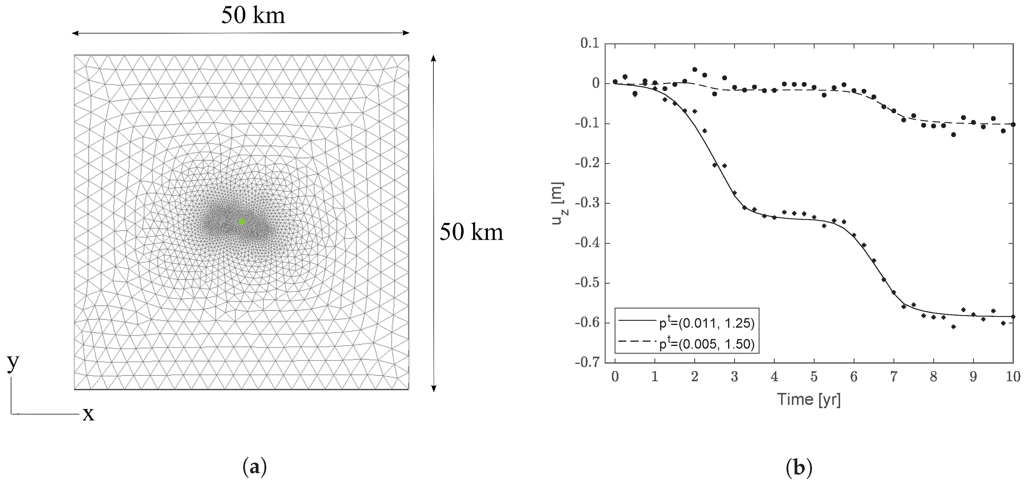
3.1. Model Set-Up and Random Parameters

The proposed approach is tested in a realistic geomechanical analysis concerning the development of a production program from a synthetic hydrocarbon reservoir. For the sake of realism, the model is built by introducing some of the typical features of the off-shore reservoirs buried in the Northern Adriatic basin, Italy [9,10,53].

The model domain covers an area of 50 km × 50 km and extends down to 5 km depth. It is discretized into the 3-D FE mesh shown in Figure 1a consisting of 71,734 nodes and 410,030 tetrahedrons. The rock in the reservoir and the hydraulically connected aquifer has a strongly non-linear visco-elasto-plastic behaviour described by the VN model, while the overburden and the underburden, that is the portions of the domain that are not filled by color in Figure 1a, are linear elastic. Homogeneous essential conditions apply on the outer and the bottom boundaries, with the top of the domain modeled as a traction-free surface. We assume the hydrocarbon production program from the reservoir to last for 3 years, then start again after a 2-year stop and be completed after 7 years, with the monitoring continuing for 3 additional years after the production stop. The average pressure variation occurring within the reservoir in time is shown in Figure 1b. The pressure distribution in space, also within the connected aquifer, is predicted by means of a dynamic reservoir flow model. The reader can refer to Reference [13] for more details.

Model uncertainty is connected to the four parameters of the material constitutive law mentioned in Section 2.1. Based on physical considerations and a possible prior knowledge, if available, a range of variability is associated to such parameters. In particular, we set:

$$\left\{\begin{array}{c}1.ln\left({\lambda }^{*}\right)\sim \mathcal{U}\left(-5.60;-4.28\right)\hfill \\ 2.{\rho }_{\kappa }\sim \mathcal{U}\left(5;20\right)\hfill \\ 3.{\rho }_{\mu }\sim \mathcal{U}\left(40;80\right)\hfill \\ 4.R\sim \mathcal{U}\left(1.2;1.5\right)\hfill \end{array}\right.$$

(28)

The range for ${\lambda }^{*}$ has been chosen recalling the physical relationship between ${\lambda }^{*}$ and the vertical compressibility $c_m$, which has been derived in References [9,53] for the Northern Adriatic basin. For the other parameters typical values reported in the literature, for example in Reference [3], have been taken into account. Hence, we initialize the gPCE algorithm by defining a vector of $n=4$ random parameters $\mathit{p}=({\lambda }^{*},{\rho }_{\kappa },{\rho }_{\mu },R)$. Note that since we employ uniform distributions for the random variables, the Legendre polynomials are used as gPCE basis functions. All the other modelling assumptions, including initial and boundary conditions, geometry and pressure distribution, are considered as deterministic.

As quantities of interest, collected in the vector $\mathit{U}$ given as output from the full forward geomechanical model $\mathcal{S}$, we consider the time series of the vertical displacement at a single-point of the top surface showed in Figure 2a, corresponding to land subsidence in time. Measurements of this quantity are supposed to be collected every three months for ten years, for example, by a GPS station. The true observations are collected in the vector ${\mathit{d}}^t$. They are synthetically obtained by running the forward model with what is assumed to be the true material parameter set (continuous lines in Figure 2b). Then, the observation vector $\mathit{d}$ is obtained by adding an error $ϵ$ sampled from a zero-mean Gaussian noise with standard deviation ${\sigma }_{ϵ}$ = 0.01 m (dots and squares in Figure 2b).

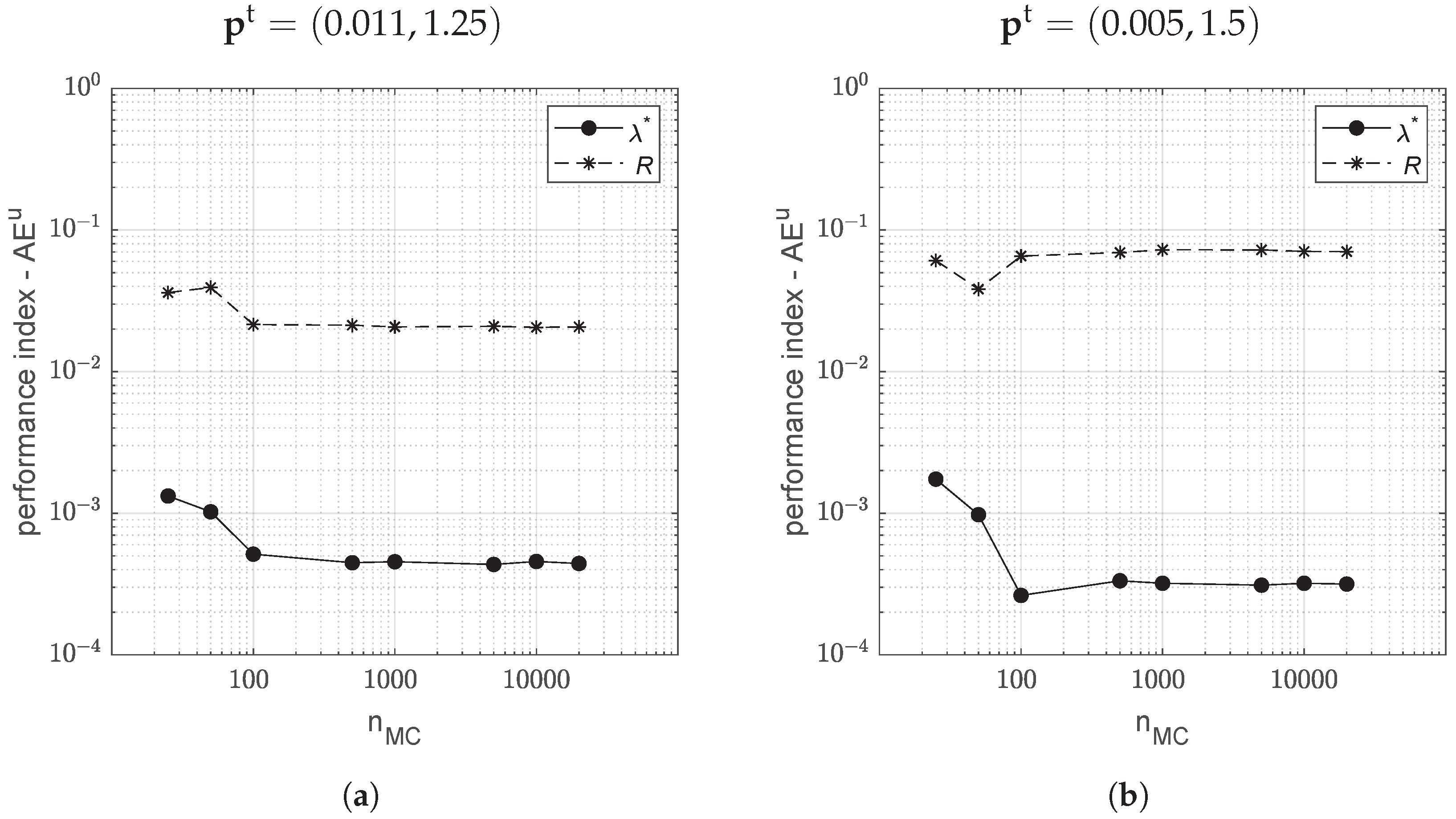
3.2. gPCE Surrogate Model

Since we use uniform distributions for the input parameters, the gPCE basis functions are multivariate Legendre polynomials, which are orthogonal with respect to the uniform measure. The first objective of this analysis is to test the quality of gPCE as a surrogate of the exact outcome of the forward model. We provide results for different degrees of the polynomial truncation, $N=$1,2,3. A full tensor approach is used for $N=1$ and $N=2$, leading to a total number $n_q$ of forward model runs equal to 16 and 81, respectively. Since with $N=3$ we would have needed $n_q=256$ full model runs, a sparse grid approach based on Smolyak’s coarse tensorization [54] is used, thus reducing $n_q$ to 137. It should be noticed that the use of such sparse grid numerical integration might lead to unacceptable errors in the expansion coefficients with higher order polynomials [55]. This issue is not encountered in the present application, however alternative accurate approaches can be also employed if needed, such as those advanced in References [55,56].

A quantitative evaluation of the fitting quality of the gPCE surrogate is provided by employing the leave-one-out (LOO) cross-validation [57,58], where an estimate of the mean-square error of the residuals between the full model and surrogate solution is given by the SSE${}_{\mathrm{LOO}}$ defined as:

$${\mathrm{SSE}}_{\mathrm{LOO}}=\frac{1}{n_q}\sum _{i=1}^{n_q}{({\mathrm{u}}_{z,i}-{\widehat{\mathrm{u}}}_{z,i}^{\sim i})}^2,$$

(29)

where ${\mathrm{u}}_{z,i}$ is the full model result at a certain time t and parameter combination i and ${\widehat{\mathrm{u}}}_{z,i}^{\sim i}$ is the surrogate solution at the same t and i with the gPCE built without the point denoted by i. In practice, the $n_q$ residuals can be obtained without building $n_q$ different gPCE but using the original gPCE constructed with the whole set of collocation points [57]. The coefficient Q${}^2$, similar to the coefficient of determination R${}^2$, can be defined as:

$${\mathrm{Q}}^2=1-\frac{{\mathrm{SSE}}_{\mathrm{LOO}}}{\mathrm{SST}},$$

(30)

where SST is the sum of the squared deviations of ${\mathrm{u}}_{z,i}$ from their mean values ${\mu }_u$ at the instant t. Values of Q${}^2$ close to 1.0 indicates a good match between the model outcome and the gPCE surrogate approximation.

Table 1. Mean ${\mu }_u$, variance ${\sigma }_u^2$ and coefficient Q${}^2$ with the generalized Polynomial Chaos Expansion (gPCE) approximation up to degree $N=1$, $N=2$ and $N=3$ (sparse grid).

	$\mathit{N}=1$ (${\mathit{n}}_{\mathit{q}}$ = 16)				$\mathit{N}=2$ (${\mathit{n}}_{\mathit{q}}$ = 81)				$\mathit{N}=3$ (${\mathit{n}}_{\mathit{q}}$ = 137)
t [yr]	${\mathit{\mu }}_{\mathit{u}}$ [m]	${\mathit{\sigma }}_{\mathit{u}}^2$ [m${}^2$]	Q${}^2$		${\mathit{\mu }}_{\mathit{u}}$ [m]	${\mathit{\sigma }}_{\mathit{u}}^2$ [m${}^2$]	Q${}^2$		${\mathit{\mu }}_{\mathit{u}}$ [m]	${\mathit{\sigma }}_{\mathit{u}}^2$ [m${}^2$]	Q${}^2$
1	−2.1× 10${}^{-3}$	2.0× 10${}^{-6}$	0.820		−2.3× 10${}^{-3}$	3.1× 10${}^{-6}$	0.931		−2.3× 10${}^{-3}$	3.0× 10${}^{-6}$	0.823
5	−1.7× 10${}^{-1}$	1.4× 10${}^{-2}$	0.860		−1.7× 10${}^{-1}$	1.5× 10${}^{-2}$	0.995		−1.7× 10${}^{-1}$	1.5× 10${}^{-2}$	0.999
10	−3.6× 10${}^{-1}$	2.6× 10${}^{-2}$	0.904		−3.7× 10${}^{-1}$	2.8× 10${}^{-2}$	0.999		−3.7× 10${}^{-1}$	2.8× 10${}^{-2}$	1.000

reports the mean and variance of vertical displacements at the times $t=$1, 5, and 10 years, along with the Q${}^2$ value. Q${}^2$ progressively increases to the upper limit of 1 for increasing N, proving the convergence of both the polynomial expansion and the high-dimensional quadrature formula. This holds true for t > 5 years with a gPCE-surrogate solution less accurate at the onset of the simulation.

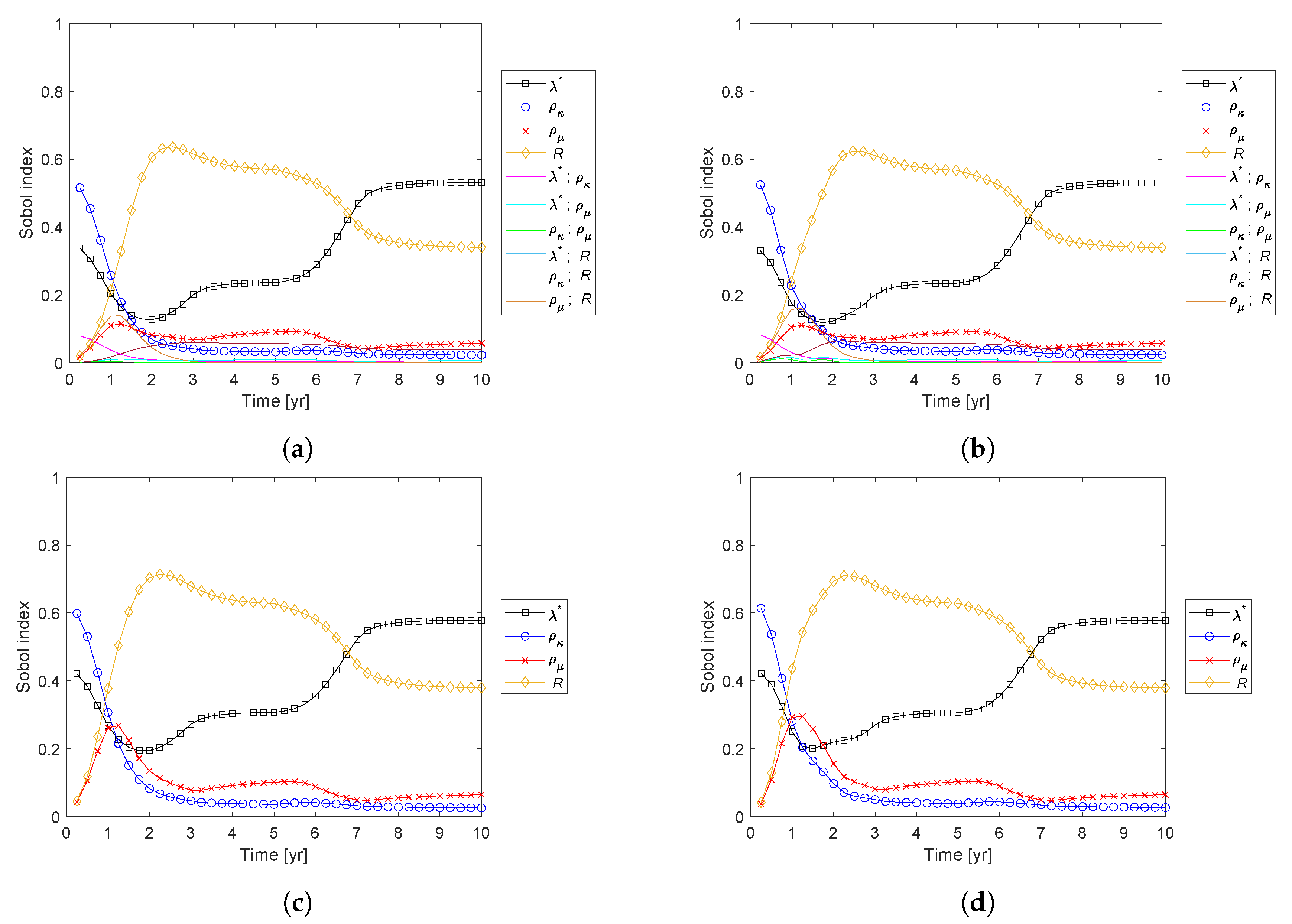
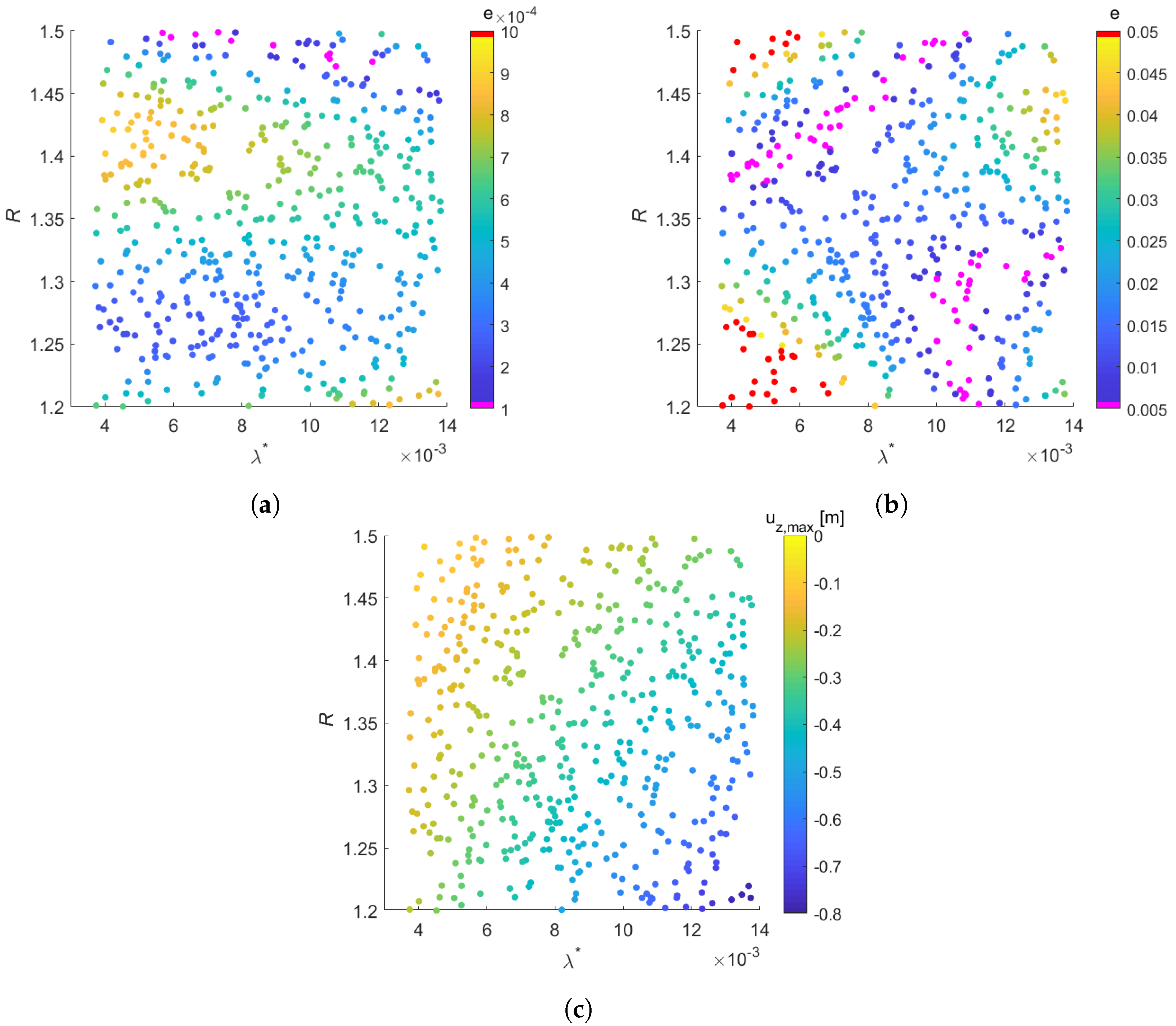
3.3. Sensitivity Analysis

Before proceeding with the assimilation, it is important to evaluate the actual influence of the uncertain parameters on the model output. We compute the Sobol’ indices using the gPCE-surrogate solution of the model output. The results are presented in Figure 3. First-order indices clearly show the higher impact on the total variance with a negligible influence of the factors interactions. In particular, parameters ${\lambda }^{*}$ and R appear to have the major impact on the solution at several times, except for the first two years where ${\rho }_{\kappa }$ and ${\rho }_{\mu }$ have a non-negligible effect. However, the significance of the quantity of interest, that is, vertical displacements, is quite limited at the beginning of the production period, because both the pressure variation and the geomechanical answer of the system are still very small and possibly influenced by the measurement errors. Thus, we limited our sensitivity analysis to the time interval between 3 and 10 years. In this temporal window, based on the total Sobol’ indices $S_{T,i}$ (Figure 3c,d) and setting ${\epsilon }_S=0.1$, we can remove from the parameter space the ratios ${\rho }_{\kappa }$ and ${\rho }_{\mu }$. However, it is important to point out that further analysis may be needed in order to investigate the model sensitivity based on different metrics, for example, on the expected value, skewness and kurtosis [59,60]. This may be helpful to better understand the role of each parameter, thus ensuring its exclusion from the parameter space is negligible.

The new parameter space is defined by $\mathit{p}=({\lambda }^{*},R)$ with $n=2$. This allows to reduce significantly the computational effort and, for the further analysis, retain the gPCE order to $N=3$ with a total number of high-dimensional quadrature nodes $n_q$ = 16. The Sobol’ indices for this new parameter space have the same behaviour as the one shown in Figure 3.

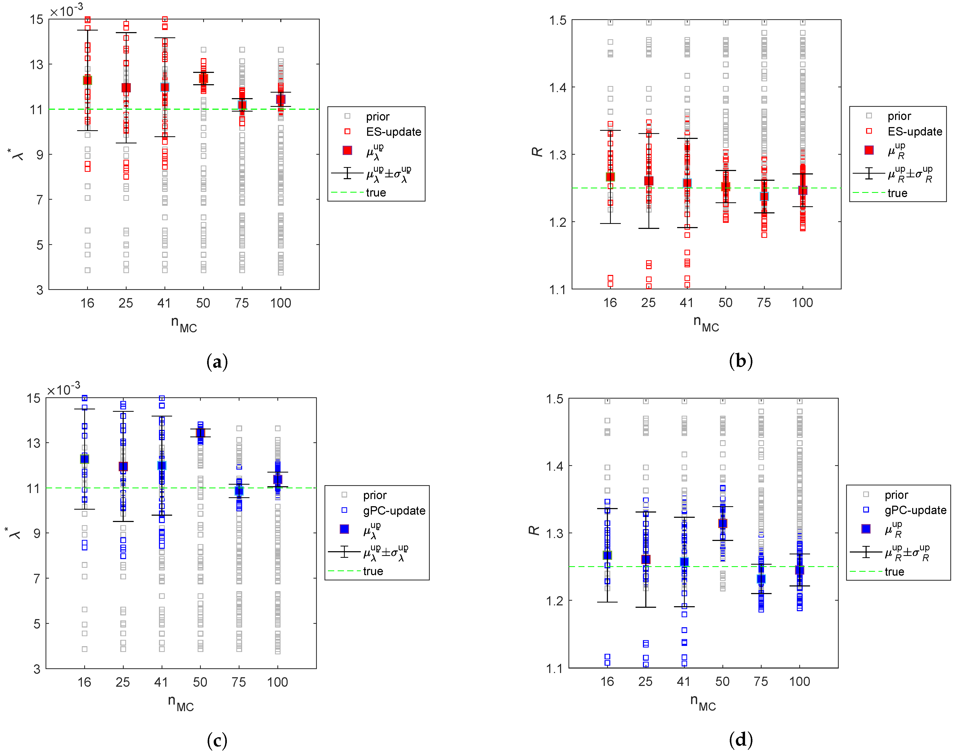
3.4. Bayesian Update

In this section, we compare the results of state/parameter update by the assimilation of surface displacements using the classical ES approach and its variation in the form of gPCE-ES. As already mentioned before, the synthetic “true” observations ${\mathit{d}}^t$ are collected from a geomechanical model run with the “true” parameter set and perturbed by a zero-mean Gaussian noise $ϵ$ (Figure 2b). Different “true” parameter sets are investigated to test the robustness of the proposed approach. The gPCE-ES technology is then applied within the iterative ES-MDA framework using either constant and decreasing factors ${\alpha }_{MDA}$ to inflate the covariance matrix of measurement error.

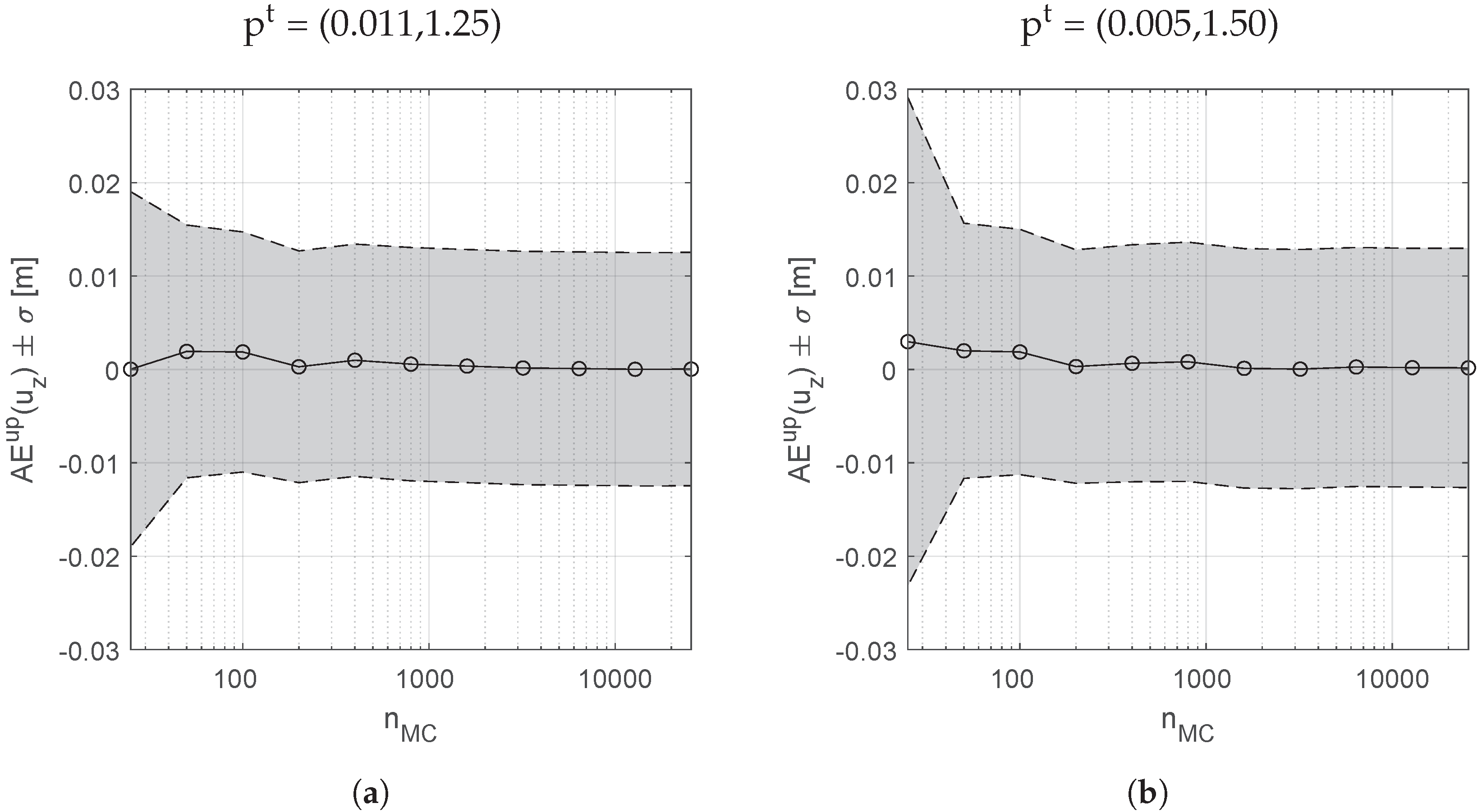
3.4.1. ES and gPCE-ES

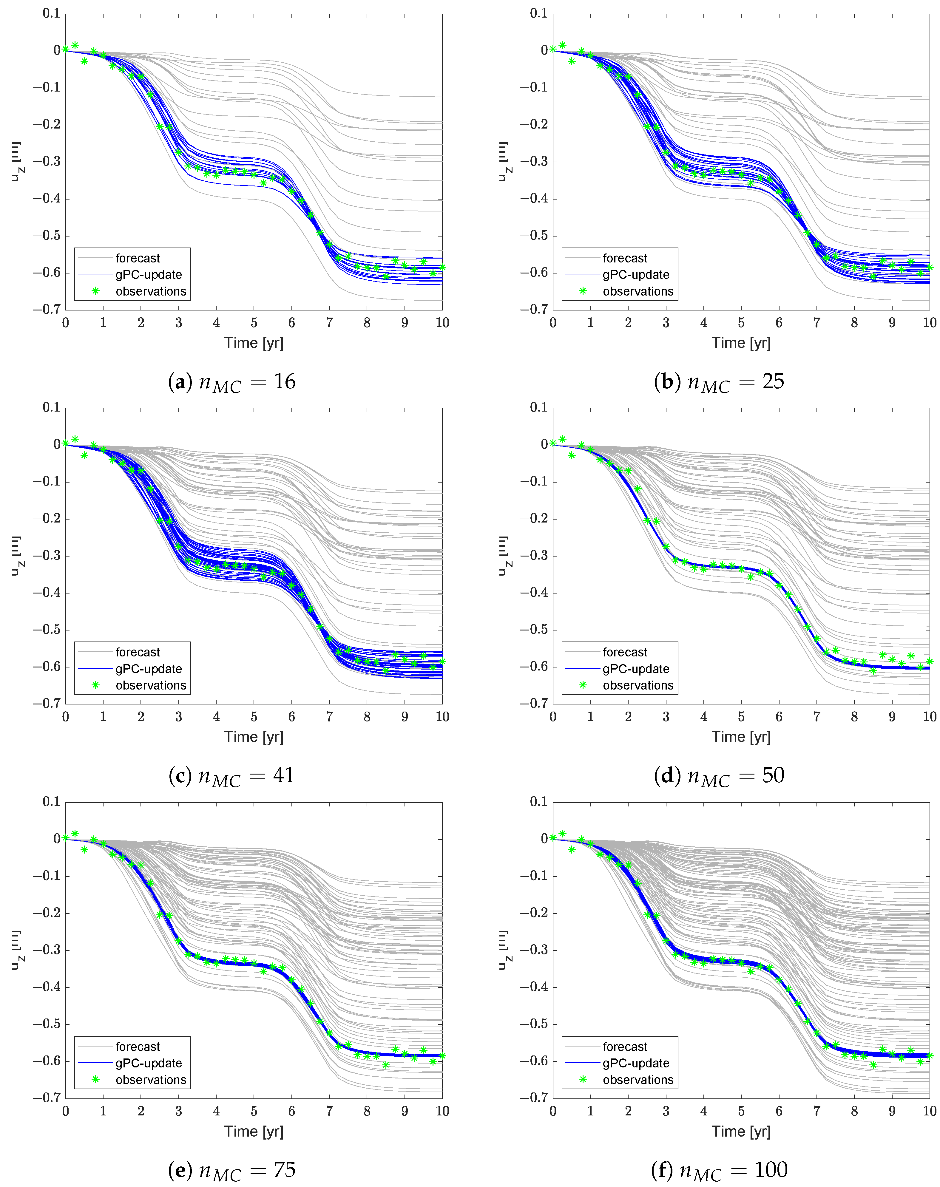
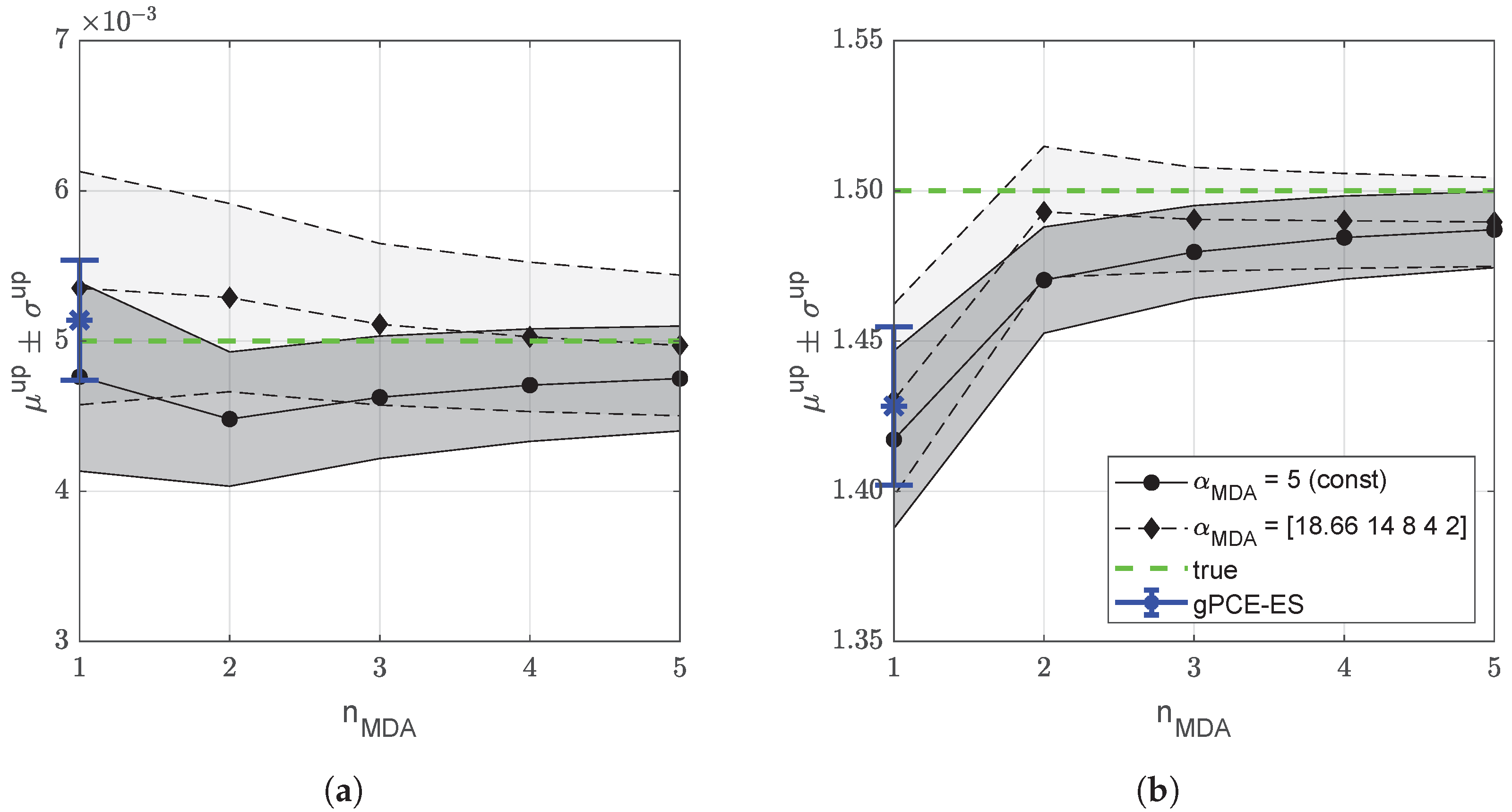
We assimilate a time series of vertical displacements collected at a point on the top surface located approximately at the center of the reservoir (Figure 2a). The synthetic observations are given by the geomechanical model run with what we assume to be the “true” parameter set $({\lambda }^{*}=0.011,R=1.25)$. The purpose is to constrain the forecast response of both state variables, for example, surface displacements and material parameters.

Figure 4 shows the prior and updated ensembles of the uncertain parameters, ${\lambda }^{*}$ (left sub-panels) and R (right sub-panels), obtained by progressively increasing the number of MC realizations. The assimilation is carried out by both the standard ES with the full forward model (red dots) and the proposed gPCE-ES approach (blue dots). As expected, the mean of the updated ensembles tends to approach the “true” value for both parameters, though with possible oscillations far from convergence, for example at $n_{MC}=50$. We provide the results for $n_{MC}=(16,25,41,50,75,100)$ in order to analyze the cases when the number of realizations is either smaller than, equal to, or larger than, the number of observations $m=41$. Since the total cost of an ES application can be regarded as roughly equal to the number of forward model runs, we can measure the computational cost, $\eta$, just by counting the number of MC simulations. Therefore, the computational cost ${\eta }_g$ associated to gPCE-ES is constant and equal to 16, that is, the number $n_q$ of forward model runs required to compute the surrogate gPCE model. By distinction, with the standard ES the computational cost, ${\eta }_f$, increases with $n_{MC}$. The uncertainty reduction is significantly improved if $n_{MC}\ge m$. In case $n_{MC}<m$ we retain 99% of the non-zero singular values computed to invert the matrix in Equation (26). Generally speaking, the parameter R better approaches the "true" value as compared to ${\lambda }^{*}$.

Figure 5 and Figure 6 show the update of the state variable ${\mathrm{u}}_z$, that is, the vertical displacement in time at the monitoring point, by increasing $n_{MC}$ with ES and gPCE-ES, respectively. The observations are generally well-captured by both approaches, with no significant differences between the methods. Hence, the proposed surrogate model appears to capture very well the overall behaviour of the forward model. To measure the quality of the approximation provided by gPCE-ES, we define the metrics AE (average error) and AES (average ensemble spread) defined as:

$$AE=\frac{1}{n_{MC}}\sum _{k=1}^{n_{MC}}|{\psi }_k-{\psi }^{true}|$$

(31)

$$AES=\frac{1}{n_{MC}}\sum _{k=1}^{n_{MC}}|{\psi }_k-{\mu }_{\psi }|,$$

(32)

where $\psi$ generally stands for state variables or parameters, and ${\mu }_{\psi }$ its mean. The metrics are computed both for prior and updated ensembles of states and parameters, providing a quantitative measure of the assimilation quality. For the state ${\mathrm{u}}_z$, time-averaged values are used to compute the metrics. AE and AES reductions (

Table 2. Values of AE and AES (prior and update) for the state and parameter ensembles computed by ES and gPCE-ES.

	ES				gPCE-ES
	${\mathit{n}}_{\mathit{MC}}=\mathbf{25}$	${\mathit{n}}_{\mathit{MC}}=\mathbf{50}$	${\mathit{n}}_{\mathit{MC}}=\mathbf{100}$		${\mathit{n}}_{\mathit{MC}}=\mathbf{25}$	${\mathit{n}}_{\mathit{MC}}=\mathbf{50}$	${\mathit{n}}_{\mathit{MC}}=\mathbf{100}$
$A{E}^p\left({\mathrm{u}}_z\right)$ [m]	0.1667	0.1642	0.1656		0.1667	0.1642	0.1656
$A{E}^u\left({\mathrm{u}}_z\right)$ [m]	0.0190	0.0104	0.0099		0.0189	0.0117	0.0101
$AE{S}^p\left({\mathrm{u}}_z\right)$ [m]	0.0834	0.0836	0.0803		0.0833	0.0836	0.0803
$AE{S}^u\left({\mathrm{u}}_z\right)$ [m]	0.0149	0.0010	0.0016		0.0149	0.0010	0.0017
$A{E}^p\left({\lambda }^{*}\right)$	0.0028	0.0029	0.0029		0.0028	0.0029	0.0029
$A{E}^u\left({\lambda }^{*}\right)$	0.0021	0.0014	0.0005		0.0021	0.0024	0.0004
$AE{S}^p\left({\lambda }^{*}\right)$	0.0027	0.0025	0.0024		0.0027	0.0025	0.0024
$AE{S}^u\left({\lambda }^{*}\right)$	0.0020	0.0002	0.0002		0.0020	0.0001	0.0003
$A{E}^p\left(R\right)$	0.1109	0.1065	0.1069		0.1109	0.1065	0.1069
$A{E}^u\left(R\right)$	0.0567	0.0186	0.0192		0.0568	0.0641	0.0184
$AE{S}^p\left(R\right)$	0.0787	0.0724	0.0729		0.0787	0.0724	0.0729
$AE{S}^u\left(R\right)$	0.0538	0.0186	0.0188		0.0538	0.0196	0.0182

) larger than 90% are obtained for both ES and gPCE-ES, thus confirming that the surrogate model is able to reproduce almost exactly the full forward model behaviour.

Based on these outcomes, we consider now only the gPCE-ES framework. Figure 7a shows the gPCE-ES convergence with $n_{MC}$. We recall that the computational cost is roughly constant, ${\eta }_g=16$. The performance index $A{E}^u$ decreases with $n_{MC}$ for both parameters and stabilizes after ∼100 $n_{MC}$. If a different “true” parameter set is used, for example, $({\lambda }^{*}=0.005,R=1.5)$, we obtain the behaviour shown in Figure 7b. In this case, the mean converges to the "true" value at a much faster rate for ${\lambda }^{*}$, while R remains poorly constrained. The “true” parameter sets are chosen such that they provide very different "true" reference simulations, as shown in Figure 2b.

3.4.2. gPCE-MDA

The ES-MDA approach is based on a multiple assimilation process to provide a better model constraint especially on strongly non-linear models. Despite the potential improvement with respect to the standard ES method, the MDA approach is rarely used in practice mainly because of the large computational cost associated to the generation of several ensembles. The introduction of an inexpensive surrogate model in place of the full forward model can make also the MDA technique more affordable in real-world problems.

We consider two test cases differing in the selection of the inflation factors ${\alpha }_{MDA}$: (i) constant ${\alpha }_{MDA}=n_{MDA}$, and (ii) decreasing ${\alpha }_{MDA}=(18.66,14,8,4,2)$. The number of successive assimilations is fixed a-priori and equal to $n_{MDA}=5$. Each assimilation step is performed by using ensembles with $n_{MC}=3000$ realizations. This ensemble size allows to achieve the convergence also with the ES technique, as shown in Figure 7. Figure 8 shows the mean and the standard deviation of the updated parameter ensembles in the five successive assimilation steps considering the “true” parameter set ${\mathbf{p}}^{\mathrm{t}}=(0.005,1.5)$. In this case, the differences with respect to a single ES assimilation (blue bar in Figure 8) are evident, that is, with multiple assimilation steps the solution appears to better approach the truth and with a reduced variability spread. This behaviour is clearly noticeable for the parameter R (Figure 8b). Similar to ES, the MDA effectiveness seems to vary when the set of observations changes. For example, with the choice of ${\mathbf{p}}^{\mathrm{t}}=({\lambda }^{*}=0.011,R=1.25)$ the improvement of multiple assimilation steps with respect to a single ES update is not significant.

The choice of the sequence of inflation factors ${\alpha }_{MDA}$ does not modify significantly the final assimilation outcome (Figure 8).

4. Discussion and Conclusions

In this work, we develop a gPCE-based framework to quantify and reduce the prediction uncertainty in geomechanical problems. The idea is to exploit the low computational cost of a gPCE-based surrogate model to—(i) perform a global sensitivity analysis and capture the material parameters mostly affecting the expected prediction, and (ii) update the variation ranges of both the state variables of interest and the governing parameters via data assimilation. We use an ensemble-based approach, such as the ES and its variation in the MDA form. Due to the high computational cost of the forward model runs required by the ensemble approaches, the proposed gPCE-ES and gPCE-MDA algorithms, if able to effectively approximate the full model behaviour, can allow for the use of large ensembles and successive assimilations at an affordable cost. The proposed approach is tested in a large-scale geomechanical model dealing with the prediction of land subsidence due to a hydrocarbon production program from a deep reservoir. To describe the constitutive behaviour of the deep rocks, we use a strongly non-linear visco-elasto-plastic model based on the VN law [3,43]. We show that high-accuracy surrogate models can be achieved via gPCE. Through the computation of the Sobol’ indices, in the specific application considered herein we demonstrate that the material parameters mainly impacting on the outcome of interest, that is, land subsidence in time, are those controlling the rock deformability in loading conditions and the size of the yield surface, ${\lambda }^{*}$ and R. The initial variability ranges of such parameters are progressively reduced through data assimilation considering: (i) standard ES, (ii) gPCE-ES, and (iii) gPCE-MDA. The gPCE-ES provides highly accurate results comparable to those obtained with the native ES approach but at a significantly lower computational cost. It is worth recalling that the high efficiency of gPCE is mostly due to the low dimension of the parameter space. In fact, the gPCE approach suffers from the so-called “curse of dimensionality” due to the exponential increase of the cost with the number of independent stochastic variables.

The gPCE-ES is used to test the ES convergence rate at an increasing size of the ensemble. By fast polynomial evaluation we can analyse ensembles up to 20,000 realizations, which are not affordable without a surrogate model. In general, the parameter mean approaches the “true” solution with increasing MC realizations. Figure 9 shows that ensemble sizes greater than ∼2000 realizations do not provide any significant improvement on the update of the state variable, that is, the mean-ensemble value of the surface displacements coincides with the observation vector. This also implies a limitation to the best match of the parameter.

We analyse the gPCE-ES convergence rate by using two parameter sets to define the “true” reference observations, with values located in the middle and on the boundary of the expected variability ranges. Different results are obtained, with a poor constraint for R when the “true” value is closer to the upper bound of the variability range. Then, we test again these sets with the gPCE-MDA approach by repeatedly assimilating the same observations a number of times with an inflated measurement error covariance matrix. We use both constant and decreasing values for the inflating factors, without any significant difference between the two approaches. The quality of the results for constraining R is significantly improved. The gPCE-MDA is obtained at the cost of computing the gPCE coefficients only, and by replacing the forward model runs required at any MDA step with fast polynomial evaluations. We demonstrate that MDA may outperform the standard ES and this option can become particularly attractive if combined with the gPCE approximation, which reduces considerably the required computational effort.

Our results show different parameter-constrain capabilities of the proposed approach depending on the choice of the reference “true” point in the parameter space. Figure 10 illustrates this behaviour in the space defined by parameters ${\lambda }^{*}$ and R. We randomly sampled 500 “true” reference parameter sets and perform the data assimilation by means of the gPCE-ES with $n_{MC}=3000$ realizations and constant noise standard error. Figure 10a,b show the error $e=|{\mu }^u-p^t|$ between the mean updated value and the true value for parameters ${\lambda }^{*}$ and R, respectively. Figure 10c shows the maximum vertical displacements assimilated at final simulation time. Clearly the ${\mathrm{u}}_{z,max}$ increases by increasing ${\lambda }^{*}$ and diminishing R. Generally, ${\lambda }^{*}$ (Figure 10a) presents higher errors with $1.35<R<1.45$ and the parameter seems to better approach the true reference value with increasing values of ${\mathrm{u}}_{z,max}$. The constrain on parameter R is more complex to analyse. A poor match is obtained at the four corners of the parameter space and minimum errors are obtained for ${\mathrm{u}}_{z,max}\simeq -0.6$ m and ${\mathrm{u}}_{z,max}\simeq -0.3$ m. Based on these results, further analyses would be needed to investigate the role of the parameter interactions on the model outcome linked to the influence of the varying time-behaviour parameter importance, with model non-linearity and measurements noise providing for additional crucial factors affecting the inverse problem solution.

References

1. Gambolati, G.; Ferronato, M.; Teatini, P.; Deidda, R.; Lecca, G. Finite element analysis of land subsidence above depleted reservoirs with pore pressure gradient and total stress formulations. Int. J. Numer. Anal. Methods Geomech. 2001, 25, 307–327. [Google Scholar] [CrossRef]
2. Spiezia, N.; Ferronato, M.; Janna, C.; Teatini, P. A two-invariant pseudoelastic model for reservoir compaction. Int. J. Numer. Anal. Methods Geomech. 2017, 41, 1870–1893. [Google Scholar] [CrossRef]
3. Isotton, G.; Teatini, P.; Ferronato, M.; Janna, C.; Spiezia, N.; Mantica, S.; Volontè, G. Robust numerical implementation of a 3D rate-dependent model for reservoir geomechanical simulations. Int. J. Numer. Anal. Methods Geomech. 2019, 43, 2752–2771. [Google Scholar] [CrossRef]
4. Lanier, J.; Caillerie, D.; Chambon, R.; Viggiani, G.; Bésuelle, P.; Desrues, J. A general formulation of hypoplasticity. Int. J. Numer. Anal. Methods Geomech. 2004, 28, 1461–1478. [Google Scholar] [CrossRef]
5. Chandong, C.; Zoback, M. Viscous creep in room-dried unconsolidated Gulf of Mexico shale (II): Development of a viscoplasticity model. J. Pet. Sci. Eng. 2010, 72, 50–55. [Google Scholar] [CrossRef]
6. Oka, F.; Kimoto, S.; Higo, Y.; Ohta, H.; Sanagawa, T.; Kodaka, T. An elasto-viscoplastic model for diatomaceous mudstone and numerical simulation of compaction bands. Int. J. Numer. Anal. Methods Geomech. 2011, 35, 244–263. [Google Scholar] [CrossRef]
7. Cassiani, G.; Brovelli, A.; Hueckel, T. A strain-rate-dependent modified Cam-Clay model for the simulation of soil/rock compaction. Geomech. Energy Environ. 2017, 11, 42–51. [Google Scholar] [CrossRef]
8. Nguyen, S.K.; Volontè, G.; Musso, G.; Brignoli, M.; Gemelli, F.; Mantica, S. Implementation of an elasto-viscoplastic constitutive law in Abaqus/Standard for an improved characterization of rock materials. In Proceedings of the 51st U.S. Rock Mechanics/Geomechanics Symposium, San Francisco, CA, USA, 25–28 June 2017. [Google Scholar]
9. Ferronato, M.; Castelletto, N.; Gambolati, G.; Janna, C.; Teatini, P. II cycle compressibility from satellite measurements. Geotechnique 2013, 63, 479. [Google Scholar] [CrossRef]
10. Zoccarato, C.; Baù, D.; Ferronato, M.; Gambolati, G.; Alzraiee, A.; Teatini, P. Data assimilation of surface displacements to improve geomechanical parameters of gas storage reservoirs. J. Geophys. Res. Solid Earth 2016, 121. [Google Scholar] [CrossRef] [Green Version]
11. Zoccarato, C.; Baù, D.; Bottazzi, F.; Ferronato, M.; Gambolati, G.; Mantica, S.; Teatini, P. On the importance of the heterogeneity assumption in the characterization of reservoir geomechanical properties. Geophys. J. Int. 2016, 207, 47–58. [Google Scholar] [CrossRef] [Green Version]
12. Fokker, P.A.; Wassing, B.B.; van Leijen, F.J.; Hanssen, R.F.; Nieuwland, D.A. Application of an ensemble smoother with multiple data assimilation to the Bergermeer gas field, using PS-InSAR. Geomech. Energy Environ. 2016, 5, 16–28. [Google Scholar] [CrossRef]
13. Gazzola, L.; Ferronato, M.; Frigo, M.; Janna, C.; Teatini, P.; Zoccarato, C.; Antonelli, M.; Corradi, A.; Dacome, M.; Mantica, S. Uncertainty quantification and reduction through Data Assimilation approaches for the geomechanical modeling of hydrocarbon reservoirs. In Proceedings of the 53rd US Rock Mechanics Geomechanics Symposium ARMA, New York, NY, USA, 23–26 June 2019. [Google Scholar]
14. Emerick, A.; Reynolds, A. Ensemble smoother with multiple data assimilation. Comput. Geosci. 2013, 55, 3–15. [Google Scholar] [CrossRef]
15. Bottazzi, F.; Della Rossa, E. A Functional Data Analysis Approach to Surrogate Modeling in Reservoir and Geomechanics Uncertainty Quantification. Math. Geosci. 2017, 49, 517–540. [Google Scholar] [CrossRef]
16. Botti, M.; Pietro, D.A.D.; Maître, O.L.; Sochala, P. Numerical approximation of poroelasticity with random coefficients using Polynomial Chaos and Hybrid High-Order methods. Comput. Methods Appl. Mech. Eng. 2019, 361, 112736. [Google Scholar] [CrossRef] [Green Version]
17. Ganesh, A.; Zhang, B.; Chalaturnyk, R.J.; Prasad, V. Uncertainty quantification of the factor of safety in a steam-assisted gravity drainage process through polynomial chaos expansion. Comput. Chem. Eng. 2020, 133, 106663. [Google Scholar] [CrossRef]
18. Castiñeira, D.; Jha, B.; Juanes, R. Uncertainty Quantification and Inverse Modeling of Fault Poromechanics and Induced Seismicity: Application to a Synthetic Carbon Capture and Storage (CCS) Problem. In Proceedings of the ARMA-2016-151, American Rock Mechanics Association, 50th U.S. Rock Mechanics/Geomechanics Symposium, Houston, TX, USA, 26–29 June 2016. [Google Scholar]
19. Zoccarato, C.; Ferronato, M.; Franceschini, A.; Janna, C.; Teatini, P. Modeling fault activation due to fluid production: Bayesian update by seismic data. Comput. Geosci. 2019, 23, 705–722. [Google Scholar] [CrossRef]
20. Verde, A. Global Sensitivity Analysis of Geomechanical Fractured Reservoir Parameters. In Proceedings of the 49th U.S. Rock Mechanics/Geomechanics Symposium, San Francisco, CA, USA, 28 June–1 July 2015; American Rock Mechanics Association: Alexandria, VA, USA, 2015. [Google Scholar]
21. Rezaei, A.; Nakshatrala, K.B.; Siddiqui, F.; Dindoruk, B.; Soliman, M. A global sensitivity analysis and reduced-order models for hydraulically fractured horizontal wells. Comput. Geosci. 2020. [Google Scholar] [CrossRef] [Green Version]
22. Wiener, N. The homogeneous chaos. Am. J. Math. 1938, 60, 897–936. [Google Scholar] [CrossRef]
23. Ghanem, R.G.; Spanos, P.D. Stochastic Finite Elements: A Spectral Approach; Springer: New York, NY, USA, 1991; (Reedited by Dover Publications: Mineola: NY, USA, 2003). [Google Scholar]
24. Xiu, D.; Karniadakis, G. The Wiener-Askey polynomial chaos for stochastic differential equations. SIAM J. Sci. Comput. 2002, 24, 619–644. [Google Scholar] [CrossRef]
25. Najm, H.N. Uncertainty Quantification and Polynomial Chaos Techniques in Computational Fluid Dynamics. Annu. Rev. Fluid Mech. 2009, 41, 35–52. [Google Scholar] [CrossRef]
26. Le Maître, O.P.; Knio, O.M. Spectral Methods for Uncertainty Quantification: With Applications to Computational Fluid Dynamics; Scientific Computation, Springer: Dordrecht, The Netherlands, 2010. [Google Scholar] [CrossRef] [Green Version]
27. Xiu, D. Numerical Methods for Stochastic Computations A Spectral Method Approach; Princeton University Press: Princeton, NJ, USA, 2010. [Google Scholar]
28. Ghanem, R. Stochastic finite elements with multiple random non-Gaussian properties. J. Eng. Mech. 1999, 125, 26–40. [Google Scholar] [CrossRef] [Green Version]
29. Sudret, B.; Berveiller, M. Stochastic finite element methods in geotechnical engineering. In Reliability-Based Design in Geotechnical Engineering: Computations and Applications; Taylor & Francis: New York, NY, USA, 2008; pp. 260–297. [Google Scholar]
30. Li, W.; Lu, Z.; Zhang, D. Stochastic analysis of unsaturated flow with probabilistic collocation method. Water Resour. Res. 2009, 45, 1–13. [Google Scholar] [CrossRef] [Green Version]
31. Fajraoui, N.; Ramasomanana, F.; Younes, A.; Mara, T.A.; Ackerer, P.; Guadagnini, A. Use of global sensitivity analysis and polynomial chaos expansion for interpretation of nonreactive transport experiments in laboratory-scale porous media. Water Resour. Res. 2011, 47, W02521. [Google Scholar] [CrossRef]
32. Oladyshkin, S.; Class, H.; Helmig, R.; Nowak, W. An integrative approach to robust design and probabilistic risk assessment for CO2 storage in geological formations. Comput. Geosci. 2011, 15, 565–577. [Google Scholar] [CrossRef]
33. Formaggia, L.; Guadagnini, A.; Imperiali, I.; Lever, V.; Porta, G.; Riva, M.; Scotti, A.; Tamellini, L. Global sensitivity analysis through polynomial chaos expansion of a basin-scale geochemical compaction model. Comput. Geosci. 2013, 17, 25–42. [Google Scholar] [CrossRef]
34. Deman, G.; Konakli, K.; Sudret, B.; Kerrou, J.; Perrochet, P.; Benabderrahmane, H. Using sparse polynomial chaos expansions for the global sensitivity analysis of groundwater lifetime expectancy in a multi-layered hydrogeological model. Reliab. Eng. Syst. Saf. 2016, 147, 156–169. [Google Scholar] [CrossRef] [Green Version]
35. Maina, F.Z.; Guadagnini, A. Uncertainty quantification and global sensitivity analysis of subsurface flow parameters to gravimetric variations during pumping tests in unconfined aquifers. Water Resour. Res. 2018, 54, 501–518. [Google Scholar] [CrossRef] [Green Version]
36. Li, J.; Xiu, D. A generalized polynomial chaos based ensemble Kalman filter with high accuracy. J. Comput. Phys. 2009, 228, 5454–5469. [Google Scholar] [CrossRef]
37. Marzouk, Y.; Xiu, D. A stochastic collocation approach to Bayesian inference in inverse problems. Commun. Comput. Phys. 2009, 6, 826–847. [Google Scholar] [CrossRef] [Green Version]
38. Saad, G.; Ghanem, R. Characterization of reservoir simulation models using a polynomial chaos-based ensemble Kalman filter. Water Resour. Res. Available online: https://0-agupubs-onlinelibrary-wiley-com.brum.beds.ac.uk/doi/epdf/10.1029/2008WR007148 (accessed on 15 May 2020). [CrossRef]
39. Oladyshkin, S.; Class, H.; Nowak, W. Bayesian updating via bootstrap filtering combined with data-driven polynomial chaos expansions: Methodology and application to history matching for carbon dioxide storage in geological formations. Comput. Geosci. 2013, 17, 671–687. [Google Scholar] [CrossRef]
40. Elsheikh, A.H.; Hoteit, I.; Wheeler, M.F. Efficient Bayesian inference of subsurface flow models using nested sampling and sparse polynomial chaos surrogates. Comput. Methods Appl. Mech. Eng. 2014, 269, 515–537. [Google Scholar] [CrossRef]
41. Biot, M.A. General theory of three-dimensional consolidation. J. Appl. Phys. 1941, 12, 155–164. [Google Scholar] [CrossRef]
42. Coussy, O. Poromechanics; John Wiley & Sons: Hoboken, NJ, USA, 2003. [Google Scholar]
43. Vermeer, P.; Neher, H. A soft soil model that accounts for creep. In Proceedings of the International Symposium “Beyond 2000 in Computational Geotechnics”, Amsterdam, The Netherlands, 18–20 March 1999; pp. 249–261. [Google Scholar]
44. Xiu, D. Efficient collocational approach for parametric uncertainty analysis. Commun. Comput. Phys. 2007, 2, 293–309. [Google Scholar]
45. Sobol’, I. Sensitivity estimates for nonlinear mathematical models. Mat. Model. 1990, 2, 112–118, (in English in Sobol’ (1993)). [Google Scholar]
46. Saltelli, A.; Marco, R.; Andres, T.; Campolongo, F.; Cariboni, J.; Gatelli, D.; Saisana, M.; Tarantola, S. Global Sensitivity Analysis. The Primer; John Wiley & Sons, Ltd.: Chichester, UK, 2007. [Google Scholar] [CrossRef]
47. Sudret, B. Global sensitivity analysis using polynomial chaos expansions. Reliab. Eng. Syst. Saf. 2008, 93, 964–979. [Google Scholar] [CrossRef]
48. Crestaux, T.; Le Maître, O.; Martinez, J.M. Polynomial chaos expansion for sensitivity analysis. Reliab. Eng. Syst. Saf. 2009, 94, 1161–1172. [Google Scholar] [CrossRef]
49. Van Leeuwen, P.; Evensen, G. Data assimilation and inverse methods in terms of a probabilistic formulation. Mon. Weather. Rev. 1996, 124, 2898–2913. [Google Scholar] [CrossRef]
50. Emerick, A.; Reynolds, A. History matching time-lapse seismic data using the ensemble Kalman filter with multiple data assimilation. Comput. Geosci. 2012, 16, 639–659. [Google Scholar] [CrossRef]
51. Emerick, A. Analysis of the performance of ensemble-based assimilation of production and seismic data. J. Pet. Sci. Eng. 2016, 139, 219–239. [Google Scholar] [CrossRef]
52. Evensen, G. Analysis of iterative ensemble smoothers for solving inverse problems. Comput. Geosci. 2018, 22, 885–908. [Google Scholar] [CrossRef] [Green Version]
53. Baù, D.; Ferronato, M.; Gambolati, G.; Teatini, P. Basin-scale compressibility of the Northern Adriatic by the radioactive marker technique. Geotechnique 2002, 52, 605–616. [Google Scholar] [CrossRef]
54. Smolyak, S.A. Quadrature and Interpolation Formulas for Tensor Products of Certain Classes of Functions. Dokl. Akad. Nauk SSSR 1963, 148, 1042–1043. [Google Scholar]
55. Constantine, P.; Eldred, M.; Phipps, E. Sparse pseudospectral approximation method. Comput. Methods Appl. Mech. Eng. 2012, 229–232, 1–12. [Google Scholar] [CrossRef] [Green Version]
56. Conrad, P.R.; Marzouk, Y.M. Adaptive Smolyak pseudospectral approximations. SIAM J. Sci. Comput. 2013, 35, A2643–A2670. [Google Scholar] [CrossRef]
57. Blatman, G. Adaptive Sparse Polynomial Chaos Expansions for Uncertainty Propagation and Sensitivity Analysis. Ph.D. Thesis, Université Blaise Pascal, Clermont-Ferrand, France, 2009. [Google Scholar]
58. Sudret, B. Polynomial chaos expansions and stochastic finite element methods. In Risk and Reliability in Geotechnical Engineering; CRC Press: Boca Raton, FL, USA, 2014; pp. 265–300. [Google Scholar]
59. Borgonovo, E. A new uncertainty importance measure. Reliab. Eng. Syst. Saf. 2007, 92, 771–784. [Google Scholar] [CrossRef]
60. Dell’Oca, A.; Riva, M.; Guadagnini, A. Moment-based metrics for global sensitivity analysis of hydrological systems. Hydrol. Earth Syst. Sci. 2017, 21, 6219–6234. [Google Scholar] [CrossRef] [Green Version]
Figure 1. (a) View of the three-dimensional finite element grid of the regional geomechanical model. The hydrocarbon reservoir is blue, while the connected aquifer is red. The vertical axis is exaggerated by a factor 3. (b) Average pore pressure variation in time within the reservoir.
Algorithms 13 00156 g001
Figure 2. (a) 2D view of the model top with the green point indicating the location where the measurements are supposed to be recorded. (b) Synthetic sequence of vertical displacements u z used in the assimilation process for two different parameter sets p t . The continuous and dashed lines are the outcomes of the geomechanical model, while dots and squares indicate the assimilated observations.
Algorithms 13 00156 g002
Figure 3. Sobol’ indices versus simulated time. Profiles with markers are used for the single parameters, while continuous profiles are used for the combinations of parameters. (a) Case with n = 4 parameters and gPCE degree N = 2 . (b) Case with n = 4 parameters and gPCE degree N = 3 with a sparse grid. (c) The same as (a) considering the total effect. (d) The same as (b) considering the total effect.
Algorithms 13 00156 g003
Figure 4. Parameter ensembles for increasing number of Monte Carlo realizations n M C . Panels (a) and (b) use the standard Ensemble Smoother (ES) with the full forward model for λ * and R, respectively. Panels (c,d) provide the same outcome as (a,b) by using the gPCE-ES approach. μ and σ are the mean and standard deviation of the updated (up) ensembles.
Algorithms 13 00156 g004
Figure 5. State ensembles for increasing number of Monte Carlo realizations n M C . In this case, the forecast ensemble (the grey one) has been obtained through the geomechanical model. The update ensemble (in red) is directly the output of the ES technique, that is, it does not derive from the geomechanical model run with the update ensembles of the parameters.
Algorithms 13 00156 g005
Figure 6. The same as Figure 5 with the forecast ensembles, in grey, obtained through the gPC expansion.
Algorithms 13 00156 g006
Figure 7. Convergence of gPCE-ES with increasing ensemble size for (a) p t = ( 0.011 , 1.25 ) and (b) p t = ( 0.005 , 1.5 ) .
Algorithms 13 00156 g007
Figure 8. Mean and standard deviation of the updated ensembles obtained with gPCE-MDA in case of constant and decreasing α M D A for parameter (a) λ * and (b) R considering the “true” parameter set p t = ( 0.005 , 1.5 ) . The blue bar refers to the results obtained with the gPCE-ES algorithm.
Algorithms 13 00156 g008
Figure 9. Mean and standard deviation for the updated displacements on the observation point varying the size of the ensembles.
Algorithms 13 00156 g009
Figure 10. Error e = | μ u p t | between the mean updated value and the true value for parameters (a) λ * and (b) R at 500 randomly-sampled ’true’ reference simulations. Sub-panel (c) shows the maximum subsidence assimilated at each assimilation.
Algorithms 13 00156 g010