On a Nonsmooth Gauss–Newton Algorithms for Solving Nonlinear Complementarity Problems


Faculty of Mathematics and Computer Science, University of Lodz, Banacha 22, 90-238 Łódź, Poland
Algorithms 2020, 13(8), 190; https://0-doi-org.brum.beds.ac.uk/10.3390/a13080190
Submission received: 25 June 2020
/
Revised: 30 July 2020
/
Accepted: 31 July 2020
/
Published: 4 August 2020
(This article belongs to the Special Issue Nonsmooth Optimization in Honor of the 60th Birthday of Adil M. Bagirov)
Abstract
:In this paper, we propose a new version of the generalized damped Gauss–Newton method for solving nonlinear complementarity problems based on the transformation to the nonsmooth equation, which is equivalent to some unconstrained optimization problem. The B-differential plays the role of the derivative. We present two types of algorithms (usual and inexact), which have superlinear and global convergence for semismooth cases. These results can be applied to efficiently find all solutions of the nonlinear complementarity problems under some mild assumptions. The results of the numerical tests are attached as a complement of the theoretical considerations.
1. Introduction
Let and let , denote the components of F. The nonlinear complementarity problem (NCP) is to find such that
The ith component of a vector is represented by . Solving (1) is equivalent to solving a nonlinear equation , where the operator is defined by
with some special function . Function may have one of the following forms:
where is any strictly increasing function with , see [1].
The (NCP) problem is one of the fundamental problems of mathematical programming, operations research, economic equilibrium models, and in engineering sciences. A lot of interesting and important applications can be found in the papers of Harker and Pang [2] and Ferris and Pang [3]. We can find the most essential applications in:
- engineering—optimal control problems, contact or structural mechanics problems, structural design problems, or traffic equilibrium problems,
- equilibrium modeling—general equilibrium (in production or consumption), invariant capital stock, or game-theoretic models.
We borrow a technique used in solving some smooth problems. If g is a merit function of G, i.e., , then any stationary point of is a least-squares solution of the equation . Then, algorithms for minimization are equivalent to algorithms for solving equations. The usual Gauss–Newton method (known also as the differential corrections method), presented by Ortega and Rheinboldt [4] in the smooth case, has the form
Local convergence properties of the Gauss–Newton method was discussed by Chen and Li [5], but only for some smooth case. The Levenberg–Marquardt method is also considered, which is a modified Gauss–Newton method, in some papers, e.g., [6] or [7]. Moreover, some comparison of semismooth algorithms for solving (NCP) problems has been made in [8].
In practice, we may also consider the damped Gauss–Newton method
with parameters and . Parameter may be chosen to ensure suitable decrease of g. If is positive for all k, then the inverse matrix in (3) always exists because is a symmetric and positive semidefinite matrix. The method (3) has the important advantage: the search direction always exists, even if is singular. Naturally, in the case of nonsmooth equations, some additional assumptions are needed to allow the use of some line search strategies and to ensure the global convergence. Because, in some cases, a function G is nondifferentiable, so the equation will be nonsmooth, whereby the method (3) may be useless. Some version of the Gauss–Newton method for solving complementarity problems was also introduced by Xiu and Zhang [9] for generalized problems, but only for linear ones. Thus, for solving nonsmooth and nonlinear problems, we propose two new versions of a damped Gauss–Newton algorithm based on B-differential. The usual generalized method is a relevant extension of the work by Subramanian and Xiu [10] for a nonsmooth case. In turn, an inexact version is related to the traditional approach, which was widely studied, e.g., in [11]. In recent years, various versions of the Gauss–Newton method were discussed, although most frequently for solving nonlinear least-squares problems, e.g., in [12,13].
The paper is organized as follows: in the next section, we review some notions needed, such as B-differential, BD-regularity, semismoothness, etc. (Section 2.1). Next, we propose a new optimization problem-based methods for the NCP, transforming the NCP into an unconstrained minimization problem by employing a function (Section 2.2). We state its global convergence and superlinear convergence rate under appropriate conditions. In Section 3, we present the results of numerical tests.
2. Materials and Methods
2.1. Preliminaries
If F is Lipschitz continuous, the Rademacher’s theorem [14] implies that F is almost everywhere differentiable. Let the set of points, where F is differentiable, be denoted by . Then, the B-differential (the Bouligand differential) of F at (introduced in [15]) is
where denotes the usual Jacobian of F at . The generalized Jacobian of F at in the sense of Clarke [14] is
We say that F is BD-regular at , if F is locally Lipschitz at and if all are nonsingular (regularity on account of B-differential). Qi proved (Lemma 2.6, [15]) that, if F is BD-regular at , then a neighborhood N of and a constant exist such that, for any and , is nonsingular and
Throughout this paper, denotes the 2-norm.
The notion of semismoothness was originally introduced for functionals by Mifflin [16]. The following definition is taken from Qi and Sun [17]. A function F is semismooth at a point , if F is locally Lipschitzian at and
exists for any . F is also said semismooth at , if it is directionally differentiable at and
Scalar products and sums of semismooth functions are still semismooth functions. Piecewise smooth functions and maximum of a finite number of smooth functions are also semismooth. The semismoothness is the almost usually seen assumption on F in papers dealing with nonsmooth equations because it implies some important properties for convergence analysis of methods in nonsmooth optimization.
If for any , as
where , then we say F is -order semismooth at . Clearly, -order semismoothness implies semismoothness. If , then the function F is called strongly semismooth. Piecewise functions are examples of strongly semismooth functions.
Qi and Sun [17] remarked that, if F is semismooth at , then, for any
and, if F is -order semismooth at , then for any
Remark 1.
Strong semismoothness of the appropriate function usually implies quadratic convergence of method instead of the superlinear one for semismooth function.
Moreover, if F is -order semismooth at , then
2.2. The Algorithm and Its Convergence
Consider nonlinear equation defined by . The equivalence of solving this equation and problem (NCP) is described by the following theorem:
Theorem 1
For the convenience, denote
for .
We assume that the function in Theorem 1 has the form
Let be the associated function. We define function g in the following way:
which allows for solving system based on solving the nonlinear least-square problem
Let us note that solves if and only if it is a stationary point of g. Thus, from Theorem 1, solves (1).
Remark 2.
On the other hand, the first-order optimality conditions for problem (6) are equivalent to the nonlinear system
where is the gradient of g, provided G is differentiable and is the Jacobian matrix of G.
The continuous differentiability of the merit function g for some kind of nonsmooth functions was established by Ulbrich in the following lemma:
Lemma 1
(Ullbrich, [19]). Assume that the function is semismooth, or, stronger, p-order semismooth, , then the merit function is continuously differentiable on D with gradient , where is arbitrary.
Lemma 2.
For any , let , where . Suppose that . Then, given , the direction given by
is an ascent direction for g. In particular, there is a positive such that .
Proof.
There exist constants and such that
because defined as is symmetric and positive semidefinite.
It follows that
Since , . If we take , we obtain
It follows that and that is a ascent direction for g (Section 8.2.1 in [4]). □
Now, we present the generalized version of the damped Gauss–Newton method for solving the nonlinear complementarity problem.
| Algorithm 1: The damped Gauss-Newton method for solving NCP |
| Let be given. Let be a starting point. Given , the steps for obtaining are: Step 1: If , then stop. Otherwise, choose any matrix and let . Step 2: Let . Step 3: Find that is a solution of the linear system |
Remark 3.
(i) In Step 2, letting is one of the simplest strategy because then converges to 0.
(ii) The line search step (Step 4) in the algorithm follows the Armijo rule.
Theorem 2.
Let be a starting point and be a sequence generated by Algorithm 1. Assume that:
(a) for all ;
(b) is Lipschitzian with a constant on the level set .
Then, the generalized damped Gauss–Newton method described by Algorithm 1 is well defined and either terminates at a stationary point of g, or else every accumulation point of , if it exists, is a stationary point of g.
Proof.
The proof is almost the same as Theorem 2.1 in [10], providing appropriately modified assumptions. □
For the nonsmooth case, the alternative condition may be considered instead of Lipschitz continuity of (similar as in [10]). Thus, we have the following convergence theorem:
Theorem 3.
Let be a starting point and be a sequence generated by Algorithm 1. Assume that:
(a) the level set is bounded;
(b) G is semismooth on .
Then, the generalized damped Gauss–Newton method described by Algorithm 1 is well defined and either terminates at a stationary point of g, or else every accumulation point of , if it exists, is a stationary point of g.
Now, we take up the rate of convergence of the considered algorithm. The following theorem shows suitable conditions in various cases.
Theorem 4.
Suppose that is a solution of problem (1), G is semismooth, and G is BD-regular at . Then, there exists a neighborhood of such that, if and the sequence is generated by Algorithm 1, we have:
(i) for all k and the sequence is linear convergent to ;
(ii) if , then the convergence is at least superlinear;
(iii) If G is strongly semismooth, then the convergence is quadratic.
Proof.
The proof of similar theorem given by Subramanian and Xiu [10] is based on three lemmas, which have the same assumptions as theorem. Now, we present these lemmas in versions adapted to our nonsmooth case. □
Lemma 3.
Assume that is a solution of the equation
where
for some matrix taken from . Then, there is a neighborhood of such that, for all
Lemma 4.
There is a neighborhood of such that, for all ,
(a) ,
(b) .
Lemma 5.
Suppose that the conditions of Lemma 1 hold. Then, there is a neighborhood of such that, for all ,
The proofs of Lemmas 5 and 6 are almost the same as in [10]; however, in the proof of Lemma 4, we have to take into account the semismoothness and to use Lemma 1 to obtain the desired result.
At the same time, in a similar way, we may show a suitable rate of convergence.
Now, we consider the inexact version of the considered method, which computes an approximate step, using the nonnegative sequence of forcing terms to control the level of accuracy.
For the above inexact version of the algorithm, we can state the analogous theorems which are equivalents of Theorems 2–4. Based on our previous results, the proof can be carried out almost in the same way as that of theorems for the ’exact’ version of the method. However, the condition (7), implied by inexactness given in Step 3 of Algorithm 2, has to be considered. Thus, we omit both theorems as proofs here.
| Algorithm 2: The inexact version of the damped Gauss-Newton method for solving NCP |
| Let and for all k given. Let be a starting point. Given , the steps for obtaining are: Step 1: If , then stop. Otherwise, choose any matrix and let . Step 2: Let . Step 3: Find that is a solution of the linear system Step 5: Compute the smallest nonnegative integer such that |
3. Numerical Results
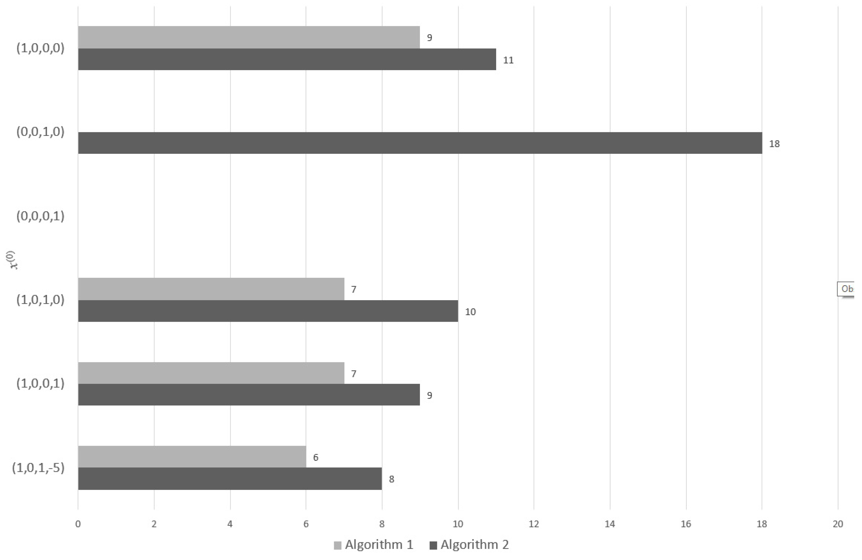
In this section, we present results of our numerical experiments, obtained by coding both algorithms in Code:Blocks. We use double precision on an Intel Core i7 3.2 GHz running under the Windows Server 2016 operating system. We applied the generalized damped Gauss–Newton method to solve three nonlinear complementarity problems. In the following examples: and denote the number of performed iterations to satisfy the stopping criterion , using Algorithms 1 and 2, respectively. The forcing terms in Algorithm 2 were chosen as follows: for all k.
Example 1
Problem (NCP) with the above function F has two solutions:
for which
Thus, is a non-degenerate solution of (NCP) because
but is a degenerate solution.
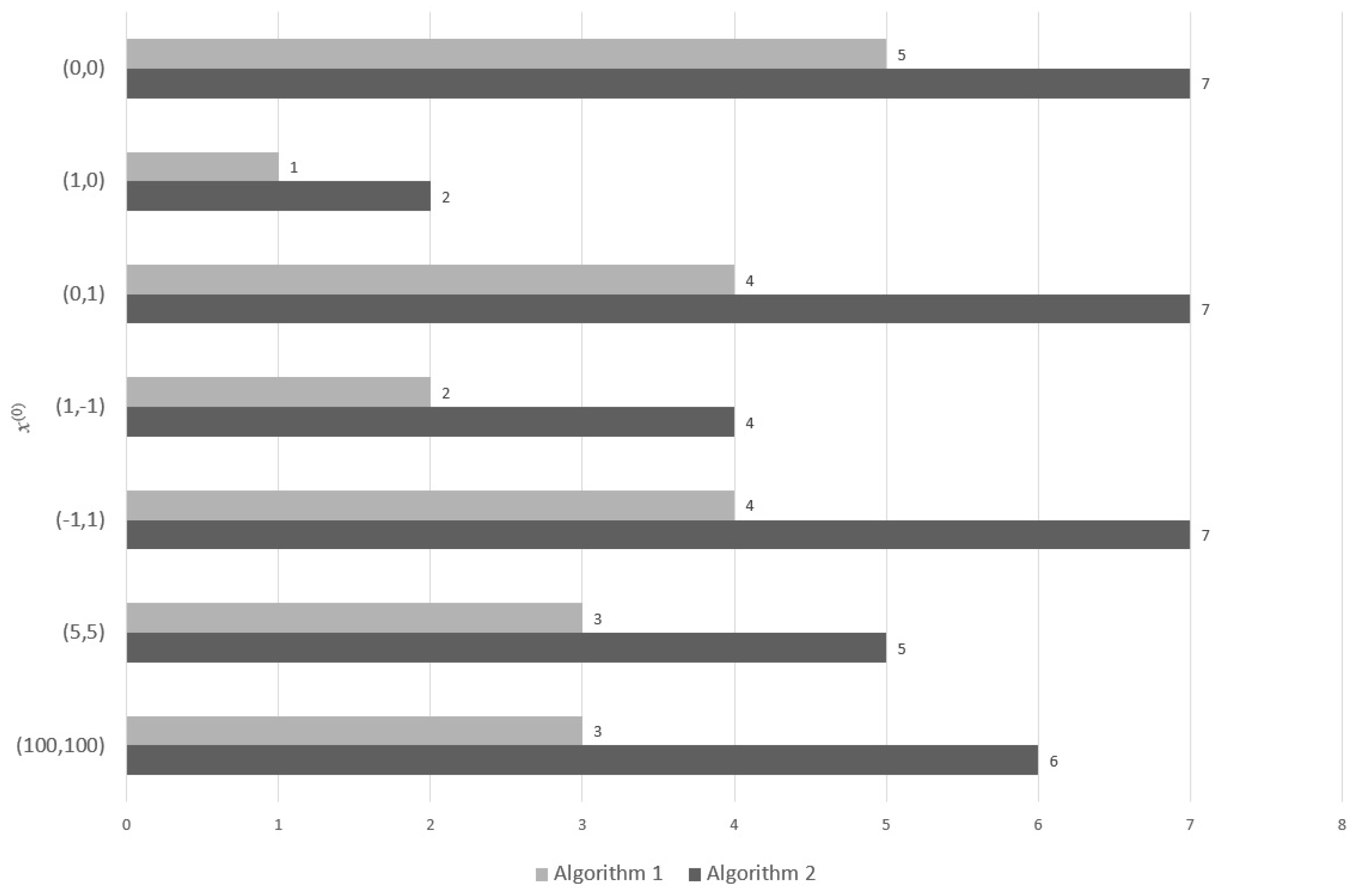
Example 2.
Let function be defined as follows:
Then, problem (NCP) has two solutions:
- -
- non-degenerate
- -
- degenerate
Example 3
Because F is strictly monotonic, the proper problem (NCP) has exactly one solution.
Calculations have been made for various n with one starting point . For all tests, we obtain the same number of iterations and .
4. Conclusions
We have given the nonsmooth version of the damped generalized Gauss–Newton method presented by Subramanian and Xu [10]. The generalized Newton algorithms related to the Gauss–Newton method are well-known important tools for solving nonsmooth equations, which arise from various nonlinear problems such as nonlinear complementarity or variational inequality. These algorithms are especially useful when the problem has many variables. We have proved that the sequences generated by the methods are superlinearly convergent under mild assumptions. Clearly, the semismoothness and BD-regularity are sufficient to obtain only a superlinear convergence of methods, while strong semismoothness even gives quadratic convergence. However, if function G is not semismooth or BD-regular or the gradient of g is not Lipschitzian, the Gauss–Newton methods may be useless.
The performance of both methods was evaluated in terms of the number of iterations required. The analysis of the numerical results seems to indicate that the methods are usually reliable for solving semismooth problems. The results show that the inexact approach can produce a noticeable slowdown by the number of iterations (compare and in Figure 1 and Figure 2). In turn, an important advantage is that the algorithms allow us to find various solutions to the problem (this can be observed in two examples: the first and second one). However, if there are many solutions of the problem, then the relationship between the starting point and the obtained solution may be unpredictable.
Clearly, traditional numerical algorithms aren’t the only method for solving the nonlinear complementarity problems, regardless of the degree of nonsmoothness. Except for the methods presented in the paper and mentioned in the Introduction, some computational intelligence algorithms can be used to solve (NCP) problems, i.a., monarch butterfly optimization (see [22,23]), the earthworm optimization algorithm (see [24]), the elephant herding optimization (see [25,26]), or the moth search algorithm (see [27,28]). All of these approaches are bio-inspired metaheuristic algorithms.
Funding
This research received no external funding.
Conflicts of Interest
The author declares no conflict of interest.
References
- Mangasarian, O.L. Equivalence of the complementarity problem to a system of nonlinear equations. SIAM J. Appl. Math. 1976, 31, 89–92. [Google Scholar] [CrossRef] [Green Version]
- Harker, P.T.; Pang, J.S. Finite-dimensional variational inequality and nonlinear complementarity problems: A survey of theory, algorithms and applications. Math. Program. 1990, 48, 161–220. [Google Scholar] [CrossRef]
- Ferris, M.C.; Pang, J.S. Engineering and economic applications of complementarity problems. SIAM Rev. 1997, 39, 669–713. [Google Scholar] [CrossRef] [Green Version]
- Ortega, J.M.; Rheinboldt, W.C. Iterative Solution of Nonlinear Equations in Several Variables; Academic Press: New York, NY, USA, 1970. [Google Scholar]
- Chen, J.; Li, W. Local convergence of Gauss–Newton’s like method in weak conditions. J. Math. Anal. Appl. 2006, 324, 381–394. [Google Scholar] [CrossRef] [Green Version]
- Fan, J.; Pan, J. On the convergence rate of the inexact Levenberg-Marquardt method. J. Ind. Manag. Optim. 2011, 7, 199–210. [Google Scholar] [CrossRef]
- Yamashita, N.; Fukushima, M. On the Rate of Convergence of the Levenberg-Marquardt Method. J. Comput. Suppl. 2001, 15, 227–238. [Google Scholar]
- De Luca, T.; Facchinei, F.; Kanzow, C.T. A theoretical and numerical comparison of some semismooth algorithms for complementarity problems. Comp. Optim. Appl. 2000, 16, 173–205. [Google Scholar] [CrossRef]
- Xiu, N.; Zhang, J. A smoothing Gauss–Newton method for the generalized HLCP. J. Comput. Appl. Math. 2001, 129, 195–208. [Google Scholar] [CrossRef] [Green Version]
- Subramanian, P.K.; Xiu, N.H. Convergence analysis of Gauss–Newton method for the complemetarity problem. J. Optim. Theory Appl. 1997, 94, 727–738. [Google Scholar] [CrossRef]
- Martínez, J.M.; Qi, L. Inexact Newton method for solving nonsmooth equations. J. Comput. Appl. Math. 1995, 60, 127–145. [Google Scholar] [CrossRef] [Green Version]
- Bao, J.F.; Li, C.; Shen, W.P.; Yao, J.C.; Guu, S.M. Approximate Gauss–Newton methods for solving underdetermined nonlinear least squares problems. App. Num. Math. 2017, 111, 92–110. [Google Scholar] [CrossRef]
- Cartis, C.; Roberts, L. A derivative-free Gauss–Newton method. Math. Program. Comput. 2019, 11, 631–674. [Google Scholar] [CrossRef] [Green Version]
- Clarke, F.H. Optimization and Nonsmooth Analysis; John Wiley & Sons: New York, NY, USA, 1983. [Google Scholar]
- Qi, L. Convergence analysis of some algorithms for solving nonsmooth equations. Math. Oper. Res. 1993, 18, 227–244. [Google Scholar] [CrossRef]
- Mifflin, R. Semismooth and semiconvex functions in constrained optimization. SIAM J. Control Optim. 1977, 15, 142–149. [Google Scholar] [CrossRef] [Green Version]
- Qi, L.; Sun, D. A nonsmooth version of Newton’s method. Math. Program. 1993, 58, 353–367. [Google Scholar] [CrossRef]
- Pang, J.S.; Qi, L. Nonsmooth equations: Motivation and algorithms. SIAM J. Optim. 1993, 3, 443–465. [Google Scholar] [CrossRef]
- Ulbrich, M. Nonmonotone trust-region methods for bound-constrained semismooth systems of equations with applications to nonlinear mixed complementarity problems. SIAM J. Optim. 2001, 11, 889–917. [Google Scholar] [CrossRef]
- Kojima, M.; Shindo, S. Extensions of Newton and quasi-Newton methods to systems of PC1-equations. J. Oper. Res. Soc. Jpn. 1986, 29, 352–374. [Google Scholar] [CrossRef]
- Jiang, H.; Qi, L. A new nonsmooth equations approach to nonlinear complementarity problems. SIAM J. Control Optim. 1997, 35, 178–193. [Google Scholar] [CrossRef]
- Feng, Y.; Wang, G.; Li, W.; Li, N. Multi-strategy monarch butterfly optimization algorithm for discounted 0–1 knapsack problem. Neural Comput. Appl. 2018, 30, 3019–3036. [Google Scholar] [CrossRef]
- Feng, Y.; Yu, X.; Wang, G. A novel monarch butterfly optimization with global position updating operator for large-scale 0–1 knapsack problems. Mathematics 2019, 7, 1056. [Google Scholar] [CrossRef] [Green Version]
- Wang, G.; Deb, S.; Coelho, L.D. Earthworm optimisation algorithm: A bio-inspired metaheuristic algorithm for global optimisation problems. Int. J. Biol. Inspired Comput. 2018, 12, 1–22. [Google Scholar] [CrossRef]
- Wang, G.; Deb, S.; Coelho, L.D. Elephant herding optimization. In Proceedings of the 2015 3rd International Symposium on Computational and Business Intelligence (ISCBI), Bali, Indonesia, 7–9 December 2015; pp. 1–5. [Google Scholar]
- Wang, G.; Deb, S.; Gao, X.; Coelho, L.D. A new metaheuristic optimisation algorithm motivated by elephant herding behaviour. Int. J. Biol. Inspired Comput. 2016, 8, 394–409. [Google Scholar] [CrossRef]
- Feng, Y.; Wang, G. Binary moth search algorithm for discounted 0-1 knapsack problem. IEEE Access 2018, 6, 10708–10719. [Google Scholar] [CrossRef]
- Wang, G. Moth search algorithm: A bio-inspired metaheuristic algorithm for global optimization problems. Memet. Comput. 2018, 10, 151–164. [Google Scholar] [CrossRef]
Figure 1.
Number of iterations for various starting points (for Example 1).

Figure 2.
Number of iterations for various starting points (for Example 2.)


Table 1.
Results for Example 1.
| x | Solution | ||
|---|---|---|---|
| 9 | 11 | ||
| failed | 18 | ||
| failed | failed | - | |
| 7 | 10 | ||
| 7 | 9 | ||
| 6 | 8 |
Table 2.
Results for Example 2.
| x | Solution | ||
|---|---|---|---|
| 5 | 7 | ||
| 1 | 2 | ||
| 4 | 7 | ||
| 2 | 4 | ||
| 4 | 7 | ||
| 3 | 5 | ||
| 3 | 6 |
© 2020 by the author. Licensee MDPI, Basel, Switzerland. This article is an open access article distributed under the terms and conditions of the Creative Commons Attribution (CC BY) license (http://creativecommons.org/licenses/by/4.0/).
Share and Cite
MDPI and ACS Style
Śmietański, M.J. On a Nonsmooth Gauss–Newton Algorithms for Solving Nonlinear Complementarity Problems. Algorithms 2020, 13, 190. https://0-doi-org.brum.beds.ac.uk/10.3390/a13080190
AMA Style
Śmietański MJ. On a Nonsmooth Gauss–Newton Algorithms for Solving Nonlinear Complementarity Problems. Algorithms. 2020; 13(8):190. https://0-doi-org.brum.beds.ac.uk/10.3390/a13080190
Chicago/Turabian StyleŚmietański, Marek J. 2020. "On a Nonsmooth Gauss–Newton Algorithms for Solving Nonlinear Complementarity Problems" Algorithms 13, no. 8: 190. https://0-doi-org.brum.beds.ac.uk/10.3390/a13080190
Note that from the first issue of 2016, this journal uses article numbers instead of page numbers. See further details here.