Deep Learning-Enabled Semantic Inference of Individual Building Damage Magnitude from Satellite Images


Geoinformatics Laboratory, School of Computing and Information, University of Pittsburgh, Pittsburgh, PA 15213, USA
*
Author to whom correspondence should be addressed.
Algorithms 2020, 13(8), 195; https://0-doi-org.brum.beds.ac.uk/10.3390/a13080195
Submission received: 11 June 2020
/
Revised: 31 July 2020
/
Accepted: 10 August 2020
/
Published: 13 August 2020
Abstract
:Natural disasters are phenomena that can occur in any part of the world. They can cause massive amounts of destruction and leave entire cities in great need of assistance. The ability to quickly and accurately deliver aid to impacted areas is crucial toward not only saving time and money, but, most importantly, lives. We present a deep learning-based computer vision model to semantically infer the magnitude of damage to individual buildings after natural disasters using pre- and post-disaster satellite images. This model helps alleviate a major bottleneck in disaster management decision support by automating the analysis of the magnitude of damage to buildings post-disaster. In this paper, we will show our methods and results for how we were able to obtain a better performance than existing models, especially in moderate to significant magnitudes of damage, along with ablation studies to show our methods and results for the importance and impact of different training parameters in deep learning for satellite imagery. We were able to obtain an overall F1 score of 0.868 with our methods.
1. Introduction
Emergency response teams draw from a large range of technical tools for the management of natural disasters [1]. Among them, the use of satellite imagery has proven highly beneficial for collecting the data required for driving detailed disaster management planning [2,3,4]. However, these satellites can gather petabytes of data [5], which is significantly more information than humans can analyze manually. Furthermore, manually analyzing such large volumes of data requires subject matter experts to derive meaning from the data [6]. For this, advanced automated methods, mainly in computer vision, are under development.
To alleviate the massive workload placed on humans for processing large amounts of satellite data, computer vision has been employed to automate the detection of objects and conditions vital to disaster management. However, despite this ability, the problem with current automated solutions is that they are unable to detect all magnitudes of damage to buildings with a high degree of confidence [7]. Therefore, while a high level of automation is possible, the current methods provide solutions at a high level of uncertainty. Furthermore, more can be done to take advantage of methods available prior to and during training to develop better performing models for computer vision satellite imagery tasks.
To fill this gap (i.e., having a model that can confidently detect all magnitudes of damage to buildings and appropriate methods prior to and during training to develop the best performing model), we propose a deep learning-based computer vision model for detecting the magnitude of damage to buildings from pre- and post-disaster images. Figure 1 shows a pipeline with the model at its core. The pipeline takes pre- and post-disaster images as input, semantically segments the buildings from the images, classifies the magnitude of damage done to each building, and provides a damage magnitude mask color-coded to label the damage detected to each building. This is novel in that current approaches reported in the literature only address the existence or the non-existence of buildings after a natural disaster or only analyze damage for a single disaster type [8,9].
Advances in deep learning have driven computer vision to new levels of performance. The creation of AlexNet, for example, noted a marked change in how computer vision tasks were approached [10], and also noted a marked change where a deep learning-based computer vision model outperformed humans on benchmark image classification tasks. For both reasons, in this paper, we propose using a convolutional neural network (CNN). CNNs also afford us many methods to apply before and during training. In our approach, we will use transfer learning, image augmentation, decaying learning rates, and class weighting. We analyze the impact of each of these methods to determine the best performing model through a series of ablation studies and experimentation.
The contribution of our paper is a deep learning-based computer vision model to semantically infer the magnitude of damage to individual buildings after natural disasters from pre-and post-disaster satellite images.
The rest of this paper will be structured as follows. We will provide a background of the problem and some related works (Section 2). We will review the dataset we will be using for our work (Section 3). We will describe the methods used for performing the work (Section 4). We will describe the experiments we performed (Section 5). We will review the results we received from our experiments (Section 6). We will discuss the results and provide analysis (Section 7). We will conclude our work and discuss some future research directions (Section 8).
2. Background
Research in computer vision and artificial intelligence focused on remote sensing in disaster management has produced a vast corpus of tools and algorithms [11] for providing the analysis and interpretation of data needed by emergency responders. Models and algorithms to infer damage or change have become increasingly popular in aiding decision support as the technology has grown to support such computation. These models and algorithms are now able to accept a range of visual inputs including satellite, drone, plane, and street view images, and can even fuse social media images for their input sources. Processing of the data can be handled with methods ranging from specific rule-based engines, to unsupervised learning techniques, to supervised machine learning techniques, and, more recently, to deep learning techniques. The output of these methods can be utilized to provide the information needed for disaster management decision support.
Identifying damage to buildings automatically from satellite images is a particularly rich field of research in remote sensing [4,8,12,13,14]. In the work of Bai et al. [14], a U-net based algorithm is used to accept pre- and post-disaster satellite images where the output is a damage detection segmentation mask. This mask provides a pixel-level classification of where buildings were either washed away, collapsed, or still standing after a Tsunami. As washed away and collapsed cases both no longer exist, this model can classify undamaged and destroyed buildings for a single disaster type with 70.9% accuracy. Cao et al. [13] used post-disaster images of buildings after a hurricane already extracted from satellite images to classify the images as damaged or undamaged using a Lenet-5-inspired CNN. They were able to achieve a 97% accuracy, but a higher accuracy is to be expected if part of the pipeline does not require identifying buildings. Doshi et al. [4] is a multi-disaster example using both flood and fire-based disasters. They used CNNs to create segmentation masks where buildings stand in pre- and post-disaster satellite images. They then took the delta of the masks to establish a change mask. Finally, they took the ratio of changed vs. unchanged pixels to establish a quantitative change ration. While this algorithm can create a true quantitative value between zero to one, it indicates changes to an area and not to specific buildings. Tu et al. [12] is one of the few examples that did not use a neural network. Instead, they used a visual bag-of-words method to create a feature-based representation of small regions in the before- and after-disaster satellite images, concatenated them, and used an SVM to make a prediction of damaged or not damaged for the small region based on the concatenated feature representations. They were able to achieve a 91.7% accuracy, but like Cao et al. [13], their work assumed knowing where buildings are. The small regions selected are not guaranteed to contain buildings at all. Lastly, Xu et al. [8] used a CNN-based architecture to detect damaged and undamaged buildings due to earthquakes. In their method, they segmented out buildings from pre- and post-disaster images and passed them into their algorithm. The algorithm extracted features of the pre- and post-disaster images, computed the delta between them, and predicted damaged or not damaged based on the delta with an AUC of 0.8302.
As mentioned in the introduction, the large strides made in deep learning-based computer vision models have made them a prime candidate for utilization in remote sensing and disaster management. Deep learning methods have been the top performers in many vision recognition tasks [15,16]. Deep learning-based methods have been shown to outperform [17,18,19] other methods in the remote sensing and disaster management space as well, including rule-based/ontological methods [6], clustering/bag-of-words methods [20], and machine learning-based methods [12]. Many of the current deep learning-based methods in the literature [7,8,13] operate on variations in CNNs. This enables them to take advantage of many powerful tools available in deep learning including image segmentation, transfer learning, class weighting, and decaying learning rates. Therefore, as part of our work, we will explore primary methods for improving the performance of and tuning such methods.
A significant advantage of CNNs is their ability to handle multi-class classification within a single model. This is another distinguishing feature between them and other methods that have been utilized in remote sensing and disaster management. Despite this, multi-class classification models for inferring damage magnitude are currently non-existent or, at best, limited in what they offer. [14] conceptualize a framework that would incorporate major damage, moderate damage, minor damage, no damage, washed away, and collapsed semantic labels. However, they only experimented with washed away, collapsed, and survived building classifications. While this is more than a binary comparison, it does not provide a measure of magnitude. The classes can simply be inferred by where a building was (label 1), where nothing is now (label 2), where a pile of rubble exist now (label 3), or where a building remains. The framework lacks the ability to determine the degree of damage to buildings that they conceptually outlined in the beginning of the paper. They also use accuracy as their measurement, which has been shown to be an inappropriate performance metric [7] as class sizes are so imbalanced in most disaster assessment cases and artificially inflate the accuracy percentage. [7] provide multi-class labels for damage magnitude (i.e., no damage, some damage, significant damage, and destroyed) and correctly choose the F1 score as their metric. However, the model is put forth as a proof of concept to complement the data model they present and only identifies no damage and destroyed cases with a significant degree of certainty.
To develop a model that could potentially be used in decision support, disaster managers require a model that can both provide multiple degrees of magnitude and do so with a moderate to high degree of certainty. This is a difficult task as degrees of magnitude between undamaged and destroyed buildings are subjective, and cases that border between two degrees of magnitude can mislead a model and complicate training [7]. The model we will develop will be trained on a satellite image dataset [21] with ground truth labels for no damage, some damage, moderate damage, and destroyed buildings. We will then use this model in a framework to provide these degrees of magnitude for buildings in a separate testing dataset with a moderate to high degree of certainty.
3. Dataset
The data used in this research are composed of high-resolution satellite images collected as part of the Maxar/DigitalGlobe data program [22]. The aim of this program is to supply satellite imagery and data to aid in response and recovery after natural disasters. To do this, the program maintains an open imagery database of satellite images that covers disasters from 2010 to the present for all types of major natural disasters world-wide. To date, the database contains collected images and data from over 50 natural disasters, which is openly available to the public.
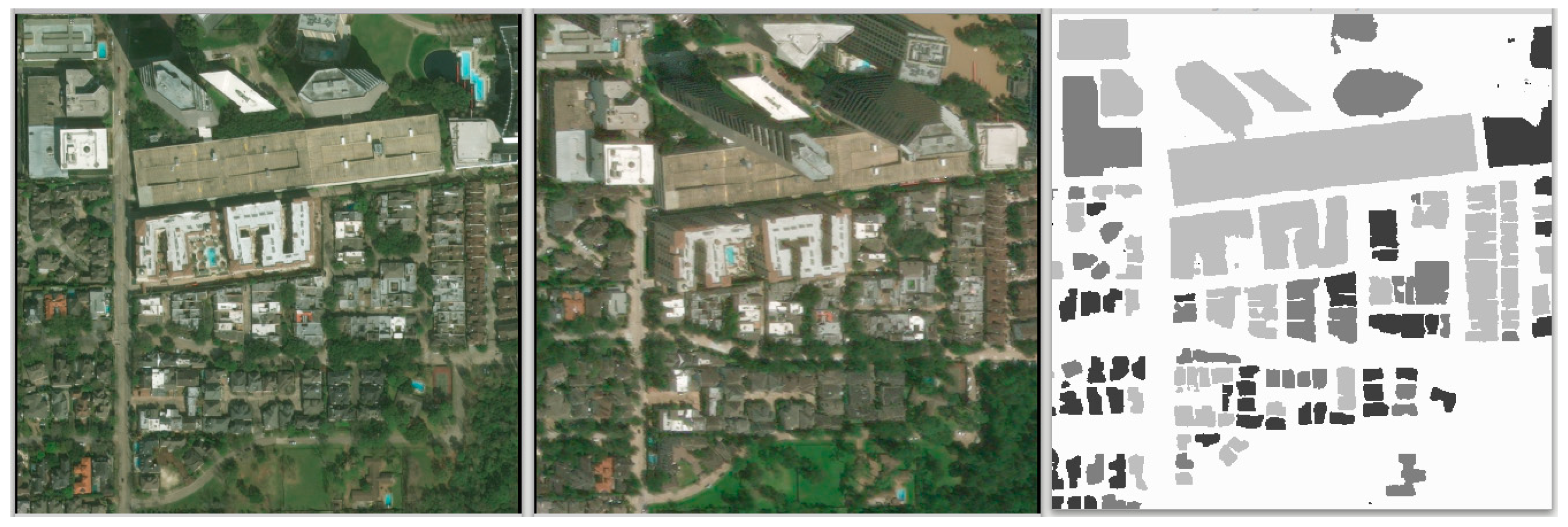
The dataset used in this work was compiled from the images in the Maxar/DigitalGlobe open data program. Images from 17 different disasters were selected. This dataset is unique from other datasets utilized in automated building damage assessment for several reasons. First, the spatial resolution for all satellite images in the dataset is under one meter. This is multiple times higher than other datasets currently available to the public. This dataset also covers multiple types of disasters, including images and data from earthquakes, tsunamis, floods, volcanic eruptions, wildfires, and wind. To the best of our knowledge, other openly available datasets only cover a single disaster type. This creates a great opportunity for developing models that can scale across different disaster types. In addition to disaster types, the dataset also features a diverse set of locations. Included in this set are images and data for disasters in the United States, Mexico, Guatemala, Portugal, Indonesia, India, and Australia. Figure 2 shows an example of one such before- and after-disaster image pair. This provides unique opportunities in disaster model development for two important reasons. First, building construction varies greatly in different parts of the world. Second, different locations vary greatly in density of buildings. Included in this dataset are images with no buildings at all, which provides data to train for the negative case, which is not offered by all datasets. These opportunities can greatly assist in creating a significantly more robust model that other datasets would allow.
An important contribution the developers of the dataset created when compiling it is the joint damage scale [7]. The description for each damage classification as provided by the creators of the dataset can be found in Table 1. The joint damage scale is a method for semantically rating the magnitude of damage to buildings across multiple types of disasters. This is an important contribution as it provides a means for equating the degree of damage to buildings regardless of the type of damage they have received. The joint damage scale uses 0 for no damage; 1 for minor damage such as some fire, water, or structural damage; 2 for major damage such as significant fire, water, or structural damage; and 3 for destroyed in cases where the building was scorched, collapsed, flooded, or missing completely. This scale was created in collaboration with the National Aeronautics and Space Administration (NASA), the California Department of Forestry and Fire Protection (CAL FIRE), the Federal Emergency Management Agency (FEMA), and the California Air National Guard [7].
The dataset was manually compiled and annotated in collaboration with the California Governor’s Office of Emergency Services (Cal OES), FEMA, the United States Geological Survey (USGS), the Carnegie Mellon University (CMU) Software Engineering Institute, the National Security Innovation Network, NASA, Cal FIRE, the California National Guard (Cal Guard), and the National Geospatial Intelligence Agency [21]. The dataset was ultimately called “xBD: A Dataset for Assessing Building Damage from Satellite Imagery” and is hosted and freely available by the Carnegie Mellon University Software engineering Institute. It covers an area of over 45,000 sq km and has annotations for over 850,000 buildings. Each building has a ground truth polygon that outlines its location in the image, and a ground truth label that assigns the building a semantic label from the joint damage scale. All images in this dataset were taken between 2011 and 2018.
4. Materials and Methods
The contribution of our paper is a deep learning-based computer vision model to semantically infer the magnitude of damage to individual buildings after natural disaster from pre- and post-disaster satellite images. This model fits into a larger pipeline that allows us to identify buildings from satellite images, infer the damage magnitude, and display the results for all buildings within the satellite image. This pipeline is composed of our best performing model, which we will call the classification model, a segmentation model that is used for identifying each building within the satellite images, and some image-based utility functions to adjust the inputs and outputs of the classification and segmentation models for each step in the pipeline appropriately.
4.1. Classification Model
As stated above, the job of the classification model that we propose is to infer the magnitude of damage to individual buildings after natural disasters. This is done by placing a deep learning-based computer vision model at the core of the model that applies labels to each building entered into the model from the joint damage scale discussed in the data section above. The best performing model was trained, validated, and tested using the deep learning algorithm along with the dataset described above in our data section. There are several key elements that are central to the training, validation, and testing for developing the best performing model, and we believe that they are important for any computer vision model being used for multi-class classification in satellite imagery. These elements include proper deep learning algorithm selection, transfer learning, class weighting, decaying learning rates, and image augmentation.
The deep learning algorithms we evaluated are all variations of classification-based neural network algorithms. Neural networks have been shown [17,18,19] to outperform prior methods in metrics such as F1 score and accuracy in classification tasks for very high-resolution satellite imagery. They are also able to collect information and draw inferences on data automatically that would otherwise require lots of manual work and subject matter expertise via other methods [6,12,20]. The algorithms evaluated were AlexNet, VGG, DenseNet, GoogLeNet, and ResNet. ResNet, in particular, is commonly cited in the literature [7] as a popular algorithm for computer vision-based tasks, including aerial imagery. These algorithms, all developed recently (between 2012 to 2016), have been shown to be competitive compared to other algorithms in standard computer vision classification benchmarks [23], and are readily available for utilization as part of the PyTorch library [24]. Another important advantage of the chosen algorithms is that PyTorch allows us to automatically pretrain the networks using networks trained on the ImageNet dataset [25]. This enables us to take advantage of transfer learning techniques from models that were carefully crafted on millions of precisely annotated images, including images of buildings.
Class weighting is a crucial element to consider whenever the classes in the ground truth do not contain an even distribution of samples. In the case of our data, the no damage semantic classification has more than eight times as many samples as any other classification. This creates a large class imbalance that can significantly bias a model toward the no damage classification. In order to resolve this issue, class weighting is applied before training to rebalance the samples so classes with a larger number of samples do not impact the model more than classes with less samples. To accomplish this, we used Equation (1) [26] to create a vector of weights and apply them to the losses generated from each class during training to remove the bias incurred by uneven class sample sizes. These weights were applied to the predicted values from the network during training to adjust the loss from the network accordingly for imbalanced classes.
Image augmentation is a proven technique [20] utilized in computer vision classification model training, but it has been underutilized in computer vision classification model training for satellite imaging. Many examples exist where no augmentation was used [17,19] and many more where only a few augmentation techniques were applied [8,16,27]. However, in deep learning libraries such as PyTorch, multiple more functions exist that allow for augmentations in a single line of code [28]. For our training, we utilized random cropping, random resizing, horizontal flipping, and vertical flipping techniques. The algorithm begins by selecting a random area between 8 and 100% of the total image and crops it to keep only the selected area. This is a technique commonly applied in computer vision [20]. It then resizes the cropped area to 224 × 224 pixels and chooses randomly whether to flip the image along the horizontal axis. Therefore, if a model is trained over 100 epochs, each sample is likely augmented in 100 slightly different ways during training, and the model is taught to recognize the ground truth for that sample from 100 different vantage points. This provides a robustness to the model that is missing from other satellite image classification models in the literature. It is highly beneficial toward preventing overfitting of a model as augmentations make the model learn more generalized features of the images on which it is training.
The last key element to highlight that is not in the literature for deep learning-based computer vision classification models for inference on satellite images is decaying learning rates [29]. Decaying learning rates is common practice in neural network algorithms, particularly in cases where stochastic gradient descent and standard loss optimization are utilized, yet this is not addressed in the literature. This is an important step in the backpropagation of many computer vision-based deep learning algorithms, especially for models trained over many epochs, as it helps adjust the step size accordingly during backpropagation while training a model. Without this technique, a model is likely to plateau at a local minimum instead of converging to a global minimum, hence producing suboptimal model performance.
4.2. Segmentation Model
The segmentation model utilized for the pipeline in our experimentation is a fork of a building segmentation model [30] adapted from the U-Net architecture [31] as part of the SpaceNet data challenge [32]. The architecture for this is a fully connected network [33]. Therefore, the images inserted into this network are down-sampled to semantically classify the most salient features in the image and then up-sampled to semantically segment all the pixels in the image from those salient features. The down-sampling happens through a series of convolutional, pooling, and activation layers common to all CNNs, but is then followed by a series of deconvolutional and unpooling layers to provide the final semantic segmentation. The output of this process will provide a mask that is a prediction provided by the network as to whether each pixel in the image is part of a building or part of the background. This prediction is evaluated by the intersection over union (IOU) of the prediction and ground truth, as shown in Equation (2). The IOU is used to determine the loss of the network for each round of training and backpropagated through the network using stochastic gradient descent.
4.3. Pipeline
As mentioned above, the pipeline is composed of the trained segmentation model, trained classification mode, and some utility functions to adjust the input and output of the models appropriately to produce our final inferred visual magnitude assessment result. Therefore, to perform a magnitude assessment inference, the pipeline begins with entering the before-disaster image into the segmentation model to find the buildings, passing the segmentation mask (location of the buildings) with the corresponding after-disaster image to the classification model, and finally using the results to display our visual representation (Figure 1).
The building segmentation process uses the trained segmentation model at its core. The before-disaster satellite image is entered as input into the model. The model will then perform a pixel-wise segmentation on the image to identify all the pixels in the image that belong to buildings. Once this is established, the segmentation process will generate corresponding polygons that will bound the identified building pixels so that we have an accurate representation of where all the buildings are located. These polygons will then be used in conjunction with the after-disaster images as input into the classification model. We will use the polygons to locate the buildings in the after-disaster images, and the classification model will provide a damage magnitude label to the buildings. The final output will be the mask with the magnitude of damage to buildings classified by lighter to darker shades of gray as the magnitude of damage increases (Figure 1).
The classification process uses the trained classification model at its core. The polygons from the segmentation process and the corresponding after-disaster images are passed into the process. The polygons are used to extract the sub images of each building from the after-disaster images. Each extracted sub-image is then fed into our trained classification model and a semantic label is inferred from each sub-image from the set of ground truth labels that exist in the dataset from the joint damage scale. The inferred semantic label and polygon are then stored in a file. The labels and polygons are then read from the file and pieced back together into a new image so that they can be color-coded by magnitude to provide an overall representation of the inferred magnitude of damage to all buildings within the image.
5. Experiments
We discuss model training for neural network algorithms through high-level and low-level experiments. There are important differences to note between the high- and low-level experiments. In the high-level experiments, the emphasis is on selecting which algorithm and parameters to use for training; no emphasis is placed on tuning. The F1 scores for the high-level experiments are recorded at the aggregate level and are also not split into individual damage magnitude classifications. The results of these high-level experiments help us understand which algorithms and parameters are effective. In the low-level experiments, the emphasis is algorithm tuning and more finite details. We focus on selecting the best training parameter values for the best performing algorithms from our high-level experiments. In the low-level experiments, we record F1 scores for each individual class as we want low-level details for selecting the final best performing model from these experiments. For the high-level experiments, we evaluate five different CNN classification algorithms with a smaller dataset to evaluate their performance and perform several rounds of high-level parameter tuning. This allows us to try many options as training and testing of the resulting models can be performed in under an hour on the Google Colab cloud server environment with GPU hardware acceleration. For the low-level experiments, we took the top performing algorithms from our initial training and ran them on the full dataset with fine parameter tuning. Training against the whole dataset required an entire day of training, so opportunities to change models and parameters were limited. Finally, we placed the top model into the larger pipeline for final model evaluation so we could measure how the model impacted the overall performance of the pipeline.
5.1. High-Level Experiments
As mentioned in our methods section, we selected AlexNet, VGG, DenseNet, GoogLeNet, and ResNet as the algorithms to evaluate our semantic classification model. These are all recent algorithms [23] that can be adapted to work well in computer vision satellite object classification tasks and are readily available in Pytorch [24]. They also fully take advantage of developments in deep learning as described in our related works section and can be used to fill the current gaps that exist in the literature for inferring damage magnitude from satellite images. All of these models also come with the option to apply pretrained weights to them from models carefully trained on the ImageNet [25] dataset. As mentioned in our methods section above, this enables us to take advantage of transfer learning techniques from models that were carefully crafted on millions of precisely annotated images, including images of buildings [25].
The data we utilized were a small random subset from the xDB [7] dataset. We chose random samples from each of the 17 different disasters uniformly. In all, we used 1000 training images, 400 validation images and 400 testing images. Each set had an equal number of images from each of the no damage, some damage, significant damage, and destroyed classification labels. Therefore, in our high-level training, no class weighting was required, and we could iterate through experiments quickly.
For the models, some parameters remained static. This choice was made for several parameters to either provide an equal comparison between models, limit the amount of time required for training and inference, or by convention. All models used cross-entropy to measure their loss and stochastic gradient descent to converge to a global minimum. Setting these metrics across all models allowed us to equally compare their outcomes and is also a convention in computer vision. All models were trained over 50 epochs with a 32-image batch size. This allowed us to create models that performed better than prior models in the literature [7] but could still be run quickly enough that we could execute many tests successively.
Of the parameters we changed, we spent the most time studying the impact that different image augmentation and learning rate techniques had on the model training process. These were parameters that we could quickly change and had a visible impact we could measure in the training loss over the first few epochs of training. We did not have to wait for all the training to complete to see if the change made a positive impact in training performance. We could not find works that included extensive use of these parameters in the literature, yet found the parameters to be the most significant ones outside of transfer learning for developing strong predictive models for semantic inference of damage magnitude in satellite imaging. In our experiments, we utilized decaying learning rates. This allowed us to decrease the step in the stochastic gradient descent procedure accordingly as we trained to avoid overshooting a global minimum and not converging. We started with a learning rate between 0.01 and 0.001 and divided the learning rate by 10 somewhere between one and four times over an entire training sequence. We adjusted the image augmentation procedure as outlined in our methods section.
5.2. Low-Level Experiments
Our low-level experimentation was like our high-level experimentation. For our detailed experimentation, we only compared the GoogleNet and ResNet algorithms. We again opted to pretrain the models to take advantage of transfer learning techniques. We also chose to continue using cross-entropy loss and stochastic gradient descent both to compare the algorithms equally and as a matter of convention. We continued to use the same image augmentation techniques for this round of experimentation as well.
We used the entire dataset for these experiments. In all, we had 114,000 training images, 24,400 validation images and 24,400 testing images. In each of the training, validation, and testing sets, there were eight times as many samples in the no damage category as any other category, so class weighting was applied for this experimentation as outlined in our methods section.
We also changed some of the other parameters accordingly. We raised the number of epochs to 100 and raised the batch size to 64. The former was to perform more robust training across all the samples, the latter to help expedite training so all training could be performed in the 12 h window allotted for running experiments on the server we used. We also chose to set the decaying learning rate to start at 0.01 and be divided by 10 a total of four times over the course of each experiment.
After completing our low-level experimentation, we placed the model we developed from the GoogleNet algorithm in our pipeline. We tested the complete pipeline using over 200 full satellite images of 1024 × 1024 pixels each. The pipeline was able to detect and semantically label the buildings appropriately and produce the desired damage magnitude images as outlined in our methods section. An example is shown in Figure 2.
6. Results
We chose to use the F1 score to measure the performance of our experiments. This choice is consistent with the literature [4,7] for inference of damage from natural disasters. In most cases, the number of samples in the undamaged classes were multiple times larger than the samples in the classes that represented damage classes in the literature [7]. This also held true for the dataset we used, where there were more than twice as many samples in the undamaged class than all the other classes containing some level of damage combined. This imbalance causes an issue when using metrics such as accuracy, which are known to be impacted by imbalanced class sizes and create inflated results as a consequence.
6.1. High-Level Experimentation
Table 2 shows the results of the initial training we performed to determine the effects of applying transfer learning, decaying learning rates, and image augmentation while training models. We performed these experiments using the ResNet algorithm. As all the subsequent training we perform in the high-level experimentation is done with CNN-based models, we would expect the application of these methods to behave similarly across all of them. Our baseline model includes all three methods, where all other models have had one of the three methods not applied to show how performance was impacted.
Table 3 provides the metrics for all the CNN algorithms we evaluated in our high-level experiments. The last row labeled “time” indicates the number of seconds on average the given algorithm required to process a single batch during the training phase. This is important not only for training a model but is a direct reflection on how long the model will require to infer the magnitude of damage to a building as well, its real-time performance. All other columns indicate the metrics aggregated for all four ground truth labels based on the weighted average. All models were trained with the transfer learning, decaying learning rates, and image augmentation parameters included.
6.2. Low-Level Experimentation
Table 4 provides the metrics for the detailed experiments we performed on the two best performing algorithms from our high-level experiments. The “class” column indicates “all” for the cases where we used the weighted average metric to measure the aggregate performance of all four classes. All other cases are labeled with the performance of the individual class directly. The “time” row again measures the number, of seconds, on average the given algorithm required to process an image during the training phase. ResNet had an equal or better metric in ten of the sixteen metrics in Table 4. For this reason, we used ResNet for the top performing model and for our pipeline experimentation in Section 6.3.
6.3. Pipeline Experimentation
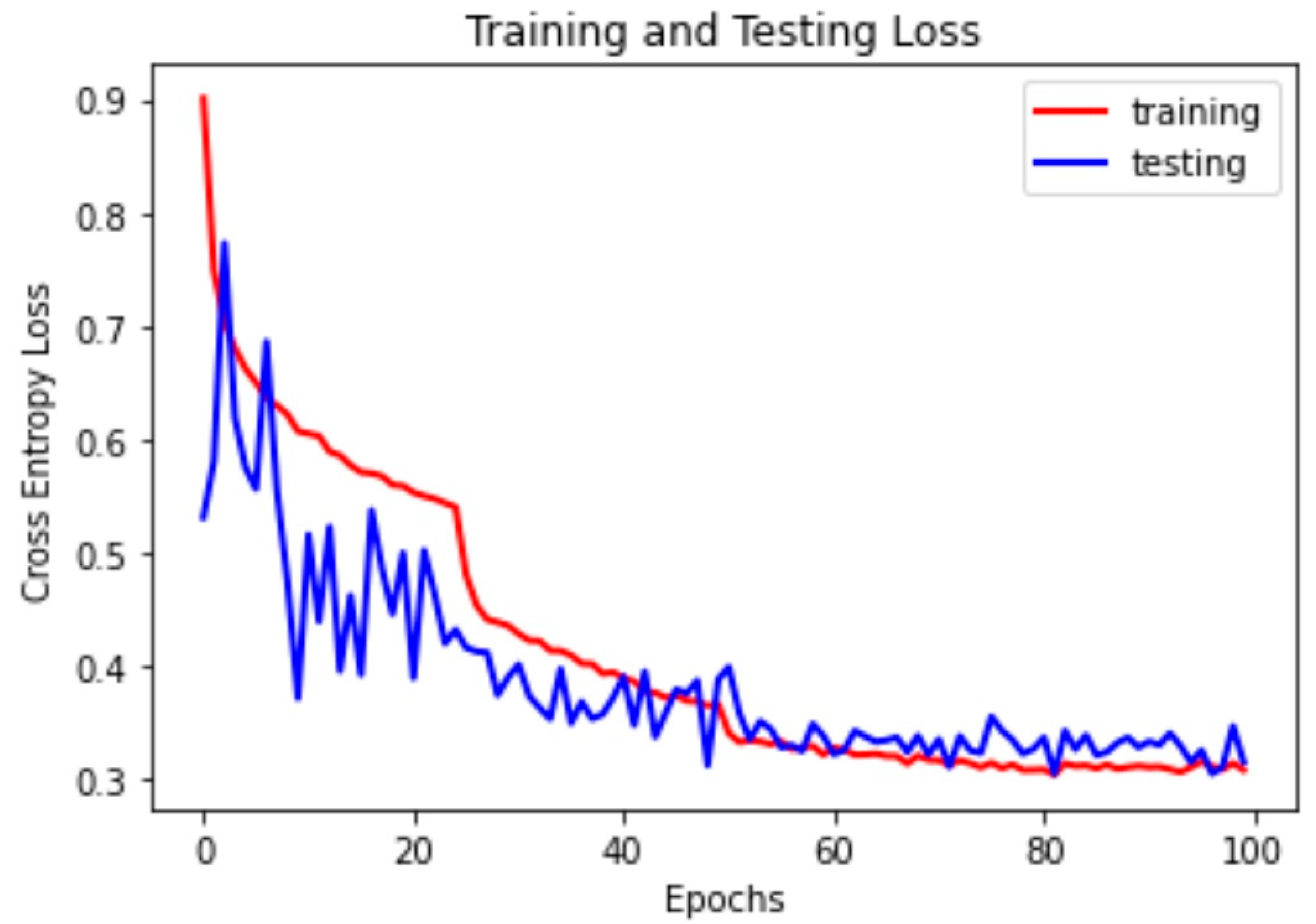
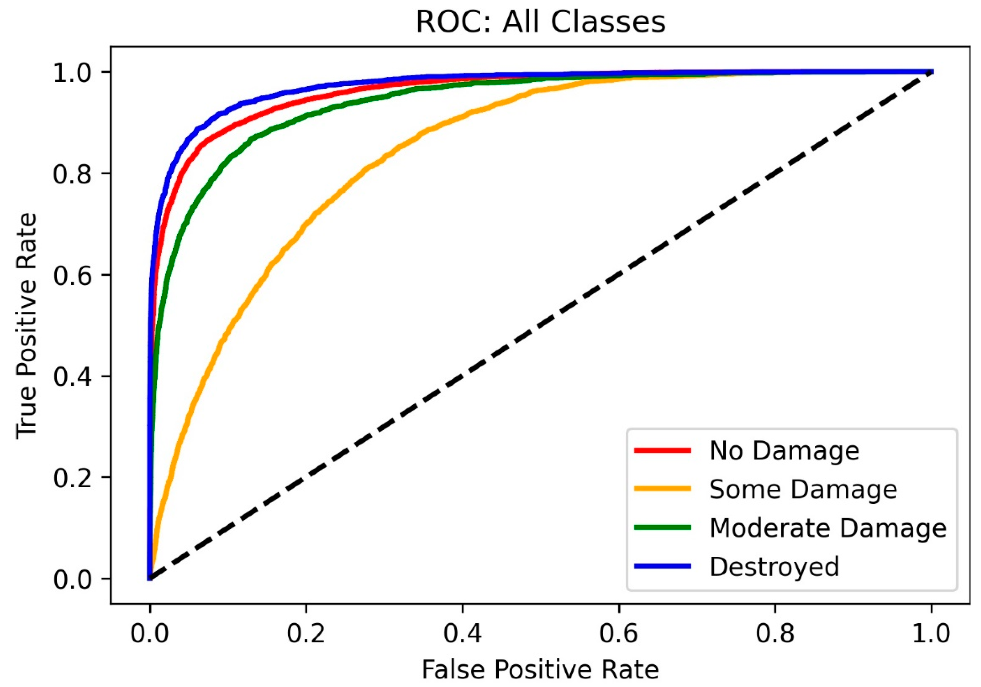
Figure 2 shows the results our final ResNet model produced when incorporated into the pipeline. The lightest shade of gray represents the buildings that were not damaged, the two darker shades of gray represent buildings with some damage and significant damage, and black represents buildings that were destroyed. Figure 3 displays the training and testing loss during our final experiments. In Figure 3, we show we were able to perform well in both training and testing phases and did not encounter overfitting in the best performing model. Additionally, we can see in Figure 4 that for all damage magnitude levels, we were able to perform well above random selection.
7. Discussion
7.1. High-Level Experimentation Analysis
As expected, transfer learning, decaying learning rates, and image augmentation helped to create a better model. Transfer learning had the largest effect on the resulting performance in our high-level experimentation. Transfer learning had the effect of enabling models to be more robust as a result of the model having already received training on millions of images from the ImageNet dataset, which included images of buildings. In this way, the best performing model was already primed to better distinguish between the shapes, colors, textures, and other features that delineated our samples into their respective classes. For similar reasons, image augmentation also proved to provide significant benefits. As a result of the cropping, zooming, and flipping methods we employed, the model was trained on a slightly different variant of the image at each epoch. For our high-level experimentation, this means that the model was trained on 50 variants of all 1000 training images. This has a large multiplicative effect and, again, greatly adds to the robustness of the model. Lastly, for any model trained with stochastic gradient descent, which most models use [19,34,35], decaying learning rates will boost performance, as shown by our experiments. Without decaying learning rates, the stochastic gradient descent process runs a greater risk of taking too large of a step near the minimum solution and consequently stepping over it. This leads to a situation where the minimum can be continually over-stepped and never reached, hence creating a situation where convergence is not reached during training and the resulting model has poorer performance. This becomes even more important as the number of epochs is raised for more sophisticated training.
Another gap in the literature is the utilization of a classification algorithm with no justification for their choice in selecting it. We avoided this issue in our work as demonstrated in Table 3. Because AlexNet is a predecessor to all the other algorithms we tested, it is not surprising that it had the lowest metrics in all categories. It is worth noting that it does run the fastest, however, so in cases where speed is of the essence, AlexNet still has value. We assume that we could achieve better performance out of both DenseNet and VGG with more individualized tuning, and they are popular options in the literature [13,27], but in an effort to keep parameters similar between algorithms so we could evaluate the algorithms equally, we did not dig deeply into individualized parameter tuning at this stage in our experimentation. This left us with both GoogleNet and ResNet as our top performers. ResNet did perform better, but it also took significantly longer to train. It is again a case where which algorithm to use will depend on the value placed on speed vs. performance metrics.
7.2. Low-Level Experimentation Analysis
As mentioned in the methods section, for the low-level experimentation, the main changes we made were that we increased from using 1000 training images to 114,000 training images, and we increased from 50 epochs to 100 epochs. We also increased from two steps to four steps when decaying the learning rate, but this was simply because we doubled the number of epochs for training. This changed our training time from under an hour to about twelve hours. This increase in performance between our high-level and low-level experiments is to be expected given the increase in samples and training resources provided.
We also noticed in our testing that the best performing model did not perform as well on the “some damage” and “moderate damage” cases. This result agrees with the observations discovered in [7], yet we were able to create models that achieved stronger predictive power across all classes than they were able to achieve as well. As mentioned before, the “some damage” and “moderate damage” cases are more subjective by their very nature compared to the “no damage” and “destroyed.” They include attributes such as some vs. moderate fire or water damage, which are hard to delineate from a machine or human perspective. These subjective measures can have a lot of room for overlap, which can create a lot of samples that are on the border between classes and would lower the reliability of the human annotated labels. By consequence, this also leaves more room for error for our trained model as well compared to the more definitive “no damage” and “destroyed” cases.
Between the algorithms we compared in our detailed experimentation, we can see that neither significantly outperformed the other in any metric. There is less than a percent difference between the models in all metrics recorded except for three of them, which are all still under 2%. The largest differences were between the metrics recorded for the recall in the “some damage” and “moderate damage” categories, where ResNet achieved higher metrics than GoogLeNet. This demonstrates another example where the “some damage” and “moderate” created the greatest challenges for the models we tested. It is worth noting that the ResNet took over 40% longer to process each image on average than the GoogLeNet algorithm. However, it is also important to note that we performed our training on the Google CoLabs servers.
8. Conclusions and Future Research Directions
In this work, we have developed a deep learning-based computer vision model to semantically infer the magnitude of damage to individual buildings after natural disasters from pre- and post-disaster satellite images. This is novel compared to other models in the literature as they do not provide any measure for the degree of damage magnitude to buildings from natural disasters. They only provide labels to tell whether a building still exists after a disaster.
Of equal importance, we outlined parameters that have a large impact in model training, particularly when using deep learning-based techniques in computer vision to generate models for inferring damage from satellite images. We found image augmentation, decaying learning rates, and transfer learning to be of high importance. This does not discount the importance of other often neglected parameters such as initial deep learning algorithm selection.
We believe that this work will pave the way for continued research in the automated assessment of damage magnitude with deep learning-based computer vision techniques. These techniques are perfectly poised to alleviate the barrier of entry imposed by other techniques requiring specialty knowledge or tools. They also alleviate many of the complicated steps required by other methods to expedite the creation of models and simplify design. In this way, one can create the solutions that will best aid the quick decision making and planning required in disaster management.
Now that we have proven we can predict the magnitude of damage to buildings with a moderate to high degree of certainty, there are several logical next steps. The first step would be to change our metric from the F1 score to the mean average precision (maP). We used F1 score for this work because it is the metric commonly used in the literature, and we wanted to use a metric that would provide a direct comparison between our work and others. However, in semantic segmentation-based models like ours, the maP is a significantly more common metric, and one that provides a better measurement of performance. In addition to measuring how well we can label buildings, the maP also measures how well we are able to locate the buildings. This will provide more meaningful information for determining the model that performs best as we are performing our training cycles.
Another opportunity exists in additional data. The dataset [21] only contains a subset of the satellite images from the original source [22]. Therefore, opportunities to extract additional training data potentially exist from these sets so we can make a stronger model. The authors of the dataset have also released an additional dataset since our experiments that we could also use for additional training.
Lastly, more complex models may prove beneficial now that we have developed a baseline model. The baseline model performs classification of damage magnitude based on the after-disaster image. More advanced algorithms exist that can provide sequential comparisons of images to learn better representations of change between images. Work with Siamese networks to directly enter and compare pre- and post-disaster images in the same network would be a logic first step in this direction.
Author Contributions
Conceptualization, B.J.W.; methodology, B.J.W.; software, B.J.W.; validation, B.J.W.; formal analysis, H.A.K.; writing—original draft preparation, B.J.W.; writing—review and editing, B.J.W. and H.A.K.; visualization, B.J.W.; supervision, H.A.K.; project administration, B.J.W. All authors have read and agreed to the published version of the manuscript.
Funding
This research received no external funding.
Conflicts of Interest
The authors declare no conflict of interest.
References
- Yu, M.; Yang, C.; Li, Y. Big data in natural disaster management: A review. Geosciences 2018, 8, 165. [Google Scholar] [CrossRef] [Green Version]
- Abdessetar, M.; Zhong, Y. Buildings change detection based on shape matching for multi-resolution remote sensing imagery. ISPRS Int. Arch. Photogramm. Remote Sens. Spat. Inf. Sci. 2017, 42, 683–687. [Google Scholar] [CrossRef] [Green Version]
- Janalipour, M.; Taleai, M. Building change detection after earthquake using multi-criteria decision analysis based on extracted information from high spatial resolution satellite images. Int. J. Remote Sens. 2016, 38, 82–99. [Google Scholar] [CrossRef]
- Doshi, J.; Basu, S.; Pang, G. From Satellite Imagery to Disaster Insights. 2018. Available online: http://arxiv.org/abs/1812.07033 (accessed on 5 May 2020).
- Albrecht, C.M.; Elmegreen, B.; Gunawan, O.; Hamann, H.F.; Klein, L.J.; Lu, S.; Mariano, F.; Siebenschuh, C.; Schmude, J. Next-Generation Geospatialtemporal Information technologies for Disaster Management. IBM J. Res. Dev. 2020, 64, 5-1. Available online: https://0-ieeexplore-ieee-org.brum.beds.ac.uk/stamp/stamp.jsp?tp=&arnumber=8977382 (accessed on 28 April 2020).
- Ghazouani, F.; Farah, I.R.; Solaiman, B. A multi-level semantic scene interpretation strategy for change interpretation in remote sensing imagery. IEEE Trans. Geosci. Remote Sens. 2019, 57, 8775–8795. [Google Scholar] [CrossRef]
- Gupta, R.; Hosfelt, R.; Sajeev, S.; Patel, N.; Goodman, B.; Doshi, J.; Heim, E.; Choset, H.; Gaston, M. xBD: A Dataset for Assessing Building Damage from Satellite Imagery. 2019. Available online: http://arxiv.org/abs/1911.09296 (accessed on 11 May 2020).
- Xu, J.Z.; Lu, W.; Li, Z.; Khaitan, P.; Zaytseva, V. Building Damage Detection in Satellite Imagery Using Convolutional Neural Networks. 2019. Available online: http://arxiv.org/abs/1910.06444 (accessed on 28 April 2020).
- Saito, K.; Spence, R.J.S.; Going, C.; Markus, M. Using high-resolution satellite images for post-earthquake building damage assessment: A study following the 26 January 2001 gujarat earthquake. Earthq. Spectra 2004, 20, 145–169. [Google Scholar] [CrossRef]
- He, K.; Zhang, X.; Ren, S.; Sun, J. Delving deep into rectifiers: Surpassing human-level performance on imagenet classification. In Proceedings of the 2015 IEEE International Conference on Computer Vision (ICCV), Santiago, Chile, 7–13 December 2015; pp. 1026–1034. [Google Scholar]
- Salah, H.S.; Goldin, S.E.; Rezgui, A.; El Islam, B.N.; Ait-Aoudia, S. What is a remote sensing change detection technique? Towards a conceptual framework. Int. J. Remote Sens. 2019, 41, 1788–1812. [Google Scholar] [CrossRef]
- Tu, J.; Li, D.; Feng, W.; Han, Q.; Sui, H. Detecting damaged building regions based on semantic scene change from multi-temporal high-resolution remote sensing images. ISPRS Int. J. Geo-Inf. 2017, 6, 131. [Google Scholar] [CrossRef] [Green Version]
- Cao, Q.D.; Choe, Y. Building damage annotation on post-hurricane satellite imagery based on convolutional neural networks. Nat. Hazards 2020, 1–20. [Google Scholar] [CrossRef]
- Bai, Y.; Mas, E.; Koshimura, S. Towards operational satellite-based damage-mapping using u-net convolutional network: A case study of 2011 tohoku earthquake-tsunami. Remote Sens. 2018, 10, 1626. [Google Scholar] [CrossRef] [Green Version]
- Girshick, R.; Donahue, J.; Darrell, T.; Malik, J.; Malik, J. Rich feature hierarchies for accurate object detection and semantic segmentation. In Proceedings of the 2014 IEEE Conference on Computer Vision and Pattern Recognition, Columbus, OH, USA, 23–28 June 2014; pp. 580–587. [Google Scholar]
- Krizhevsky, A.; Sutskever, I.; Hinton, G.E. ImageNet classification with deep convolutional neural networks. Commun. ACM 2017, 60, 84–90. [Google Scholar] [CrossRef]
- Cheng, G.; Han, J.; Lu, X. Remote sensing image scene classification: Benchmark and state of the art. Proc. IEEE 2017, 105, 1865–1883. [Google Scholar] [CrossRef] [Green Version]
- Mou, L.; Bruzzone, L.; Zhu, X.X. Learning spectral-spatial-temporal features via a recurrent convolutional neural network for change detection in multispectral imagery. IEEE Trans. Geosci. Remote Sens. 2018, 57, 924–935. [Google Scholar] [CrossRef] [Green Version]
- Nogueira, K.; Penatti, O.A.B.; Dos Santos, J.A. Towards better exploiting convolutional neural networks for remote sensing scene classification. Pattern Recognit. 2017, 61, 539–556. [Google Scholar] [CrossRef] [Green Version]
- Szegedy, C.; Liu, W.; Jia, Y.; Sermanet, P.; Reed, S.; Anguelov, D.; Erhan, D.; Vanhoucke, V.; Rabinovich, A. Going deeper with convolutions. In Proceedings of the 2015 IEEE Conference on Computer Vision and Pattern Recognition (CVPR), Boston, MA, USA, 7–12 June 2015; pp. 1–9. [Google Scholar]
- xView2. 2020. Available online: https://xview2.org/ (accessed on 27 April 2020).
- Maxar. 2020. Available online: https://www.digitalglobe.com/ecosystem/open-data (accessed on 27 April 2020).
- Singh, R.V. ImageNet Winning CNN Architectures—A Review. 2015. Available online: http://rajatvikramsingh.github.io/media/DeepLearning_ImageNetWinners.pdf (accessed on 27 April 2020).
- PyTorch Models. 2020. Available online: https://pytorch.org/docs/stable/torchvision/models.html (accessed on 27 April 2020).
- Deng, J.; Dong, W.; Socher, R.; Li, L.J.; Li, K.; Fei-Fei, L. ImageNet: A large-scale hierarchical image database. In Proceedings of the 2009 IEEE Conference on Computer Vision and Pattern Recognition, Miami, FL, USA, 20–25 June 2009. [Google Scholar]
- Sklearn Class Weighting. 2020. Available online: https://scikit-learn.org/stable/modules/generated/sklearn.utils.class_weight.compute_class_weight.html (accessed on 27 April 2020).
- Li, L.; Liang, J.; Weng, M.; Zhu, H. A multiple-feature reuse network to extract buildings from remote sensing imagery. Remote Sens. 2018, 10, 1350. [Google Scholar] [CrossRef] [Green Version]
- Torchvision Transforms. 2020. Available online: https://pytorch.org/docs/stable/torchvision/transforms.html (accessed on 15 May 2020).
- Brownlee, J. How to Configure the Learning Rate When Training Deep Learning Neural Networks. Machine Learning Mastery. 2019. Available online: https://machinelearningmastery.com/learning-rate-for-deep-learning-neural-networks/ (accessed on 6 May 2020).
- Kimura, M. GitHub-Motokimura/Spacenet_Building_Detection: Project to Train/Test Convolutional Neural Networks to Extract Buildings from Spacenet Satellite Imageries. 2020. Available online: https://github.com/motokimura/spacenet_building_detection (accessed on 27 April 2020).
- Ronneberger, O.; Fischer, P.; Brox, T. U-Net: Convolutional networks for biomedical image segmentation. Adv. Cryptol. CRYPTO 2017 2015, 9351, 234–241. [Google Scholar]
- Van Etten, A.; Lindenbaum, D.; Bacastow, T.M. SpaceNet: A Remote Sensing Dataset and Challenge Series. 2018. Available online: http://arxiv.org/abs/1807.01232 (accessed on 27 April 2020).
- Shelhamer, E.; Long, J.; Darrell, T. Fully convolutional networks for semantic segmentation. IEEE Trans. Pattern Anal. Mach. Intell. 2017, 39, 640–651. [Google Scholar] [CrossRef] [PubMed]
- Alshehhi, R.; Marpu, P.R.; Woon, W.L.; Mura, M.D. Simultaneous extraction of roads and buildings in remote sensing imagery with convolutional neural networks. ISPRS J. Photogramm. Remote Sens. 2017, 130, 139–149. [Google Scholar] [CrossRef]
- Sakrapee, P.; Jamie, S.; Pranam, J.; van den Anton, H. Semantic Labeling of Aerial and Satellite Imagery. IEEE J. Sel. Top. Appl. Earth Obs. Remote Sens. 2016, 9. Available online: https://ieeexplore-ieee-org.pitt.idm.oclc.org/stamp/stamp.jsp?tp=&arnumber=7516568 (accessed on 27 April 2020).
Figure 1.
Pipeline for classifying damage magnitude to buildings from satellite images.

Figure 2.
From left to right: The before-disaster, after-disaster, and damage magnitude inference images from our pipeline.
Figure 2.
From left to right: The before-disaster, after-disaster, and damage magnitude inference images from our pipeline.

Figure 3.
Training and testing cross-entropy loss of final ResNet model from Table 4.
Figure 3.
Training and testing cross-entropy loss of final ResNet model from Table 4.

Figure 4.
ROC curves for all four damage magnitude levels.


Table 1.
Joint damage scale classifications.
| Classification | Description |
|---|---|
| No damage | No damage indicated |
| Some damage | Minor damage such as some fire, water, or structural damage |
| Moderate damage | Major damage such as significant fire, water, or structural damage |
| Destroyed | Building scorched, collapsed, flooded, or missing completely |
Table 2.
Training with different parameters.
| Experiment | F1 Score | Precision | Recall |
|---|---|---|---|
| Baseline | 0.699 | 0.710 | 0.695 |
| No Decay | 0.639 | 0.639 | 0.640 |
| No Augmentation | 0.643 | 0.643 | 0.645 |
| No Pretraining | 0.547 | 0.552 | 0.545 |
Table 3.
Training with different algorithms.
| Metric | AlexNet | DenseNet | GoogLeNet | ResNet | VGG |
|---|---|---|---|---|---|
| F1 Score | 0.607 | 0.659 | 0.701 | 0.701 | 0.686 |
| Precision | 0.610 | 0.659 | 0.702 | 0.705 | 0.691 |
| Recall | 0.605 | 0.660 | 0.700 | 0.700 | 0.685 |
| Time | 0.219 | 0.857 | 0.234 | 0.864 | 0.626 |
Table 4.
Low-level experimentation.
| Metric | Category | GoogLeNet | ResNet |
|---|---|---|---|
| F1 Score | All | 0.868 | 0.868 |
| F1 Score | No Damage | 0.927 | 0.924 |
| F1 Score | Some Damage | 0.592 | 0.587 |
| F1 Score | Moderate Damage | 0.716 | 0.721 |
| F1 Score | Destroyed | 0.811 | 0.814 |
| Precision | All | 0.888 | 0.889 |
| Precision | No Damage | 0.977 | 0.98 |
| Precision | Some Damage | 0.489 | 0.478 |
| Precision | Moderate Damage | 0.665 | 0.666 |
| Precision | Destroyed | 0.770 | 0.772 |
| Recall | All | 0.858 | 0.855 |
| Recall | No Damage | 0.881 | 0.874 |
| Recall | Some Damage | 0.749 | 0.760 |
| Recall | Moderate Damage | 0.773 | 0.785 |
| Recall | Destroyed | 0.858 | 0.862 |
| Time | All | 0.227 | 0.388 |
© 2020 by the authors. Licensee MDPI, Basel, Switzerland. This article is an open access article distributed under the terms and conditions of the Creative Commons Attribution (CC BY) license (http://creativecommons.org/licenses/by/4.0/).
Share and Cite
MDPI and ACS Style
Wheeler, B.J.; Karimi, H.A. Deep Learning-Enabled Semantic Inference of Individual Building Damage Magnitude from Satellite Images. Algorithms 2020, 13, 195. https://0-doi-org.brum.beds.ac.uk/10.3390/a13080195
AMA Style
Wheeler BJ, Karimi HA. Deep Learning-Enabled Semantic Inference of Individual Building Damage Magnitude from Satellite Images. Algorithms. 2020; 13(8):195. https://0-doi-org.brum.beds.ac.uk/10.3390/a13080195
Chicago/Turabian StyleWheeler, Bradley J., and Hassan A. Karimi. 2020. "Deep Learning-Enabled Semantic Inference of Individual Building Damage Magnitude from Satellite Images" Algorithms 13, no. 8: 195. https://0-doi-org.brum.beds.ac.uk/10.3390/a13080195
Note that from the first issue of 2016, this journal uses article numbers instead of page numbers. See further details here.