Article

A Simheuristic Algorithm for Solving the Stochastic Omnichannel Vehicle Routing Problem with Pick-up and Delivery

by
Leandro do C. Martins
*,
Christopher Bayliss
,
Pedro J. Copado-Méndez
,
Javier Panadero
and
Angel A. Juan
Internet Interdisciplinary Institute (IN3)–Computer Science Department, Universitat Oberta de Catalunya, 08018 Barcelona, Spain
*
Author to whom correspondence should be addressed.
Submission received: 24 August 2020 / Revised: 14 September 2020 / Accepted: 15 September 2020 / Published: 19 September 2020
(This article belongs to the Special Issue Simulation-Optimization in Logistics, Transportation, and SCM)

Abstract

:
Advances in information and communication technologies have made possible the emergence of new shopping channels. The so-called ‘omnichannel’ retailing mode allows customers to shop for products online and receive them at home. This paper focuses on the omnichannel delivery concept for the retailing industry, which addresses the replenishment of a set of retail stores and the direct shipment of the products to customers within an integrated vehicle routing formulation. Due to its NP-Hardness, a constructive heuristic, which is extended into a biased-randomized heuristic and which is embedded into a multi-start procedure, is introduced for solving the large-sized instances of the problem. Next, the problem is enriched by considering a more realistic scenario in which travel times are modeled as random variables. For dealing with the stochastic version of the problem, a simheuristic algorithm is proposed. A series of computational experiments contribute to illustrate how our simheuristic can provide reliable and low-cost solutions under uncertain conditions.

1. Introduction

Today, people are changing their shopping behavior. Recent advances in information and communication technologies have introduced new shopping channels and models, which make possible the expansion of e-commerce and, consequently, the emergence of new challenges in operational research, transportation, and logistics areas. Specifically, regarding modern e-commerce business models, new decision variables and constraints have been incorporated in them, leading to emerging variants of distribution problems in supply chain management.
Unlike brick-and-mortar stores, where salespeople are available to support and help customers to make their purchases, the popularization of mobile devices with access to the Internet has promoted the use of different shopping channels. The online channel is an example that has emerged as a competitive marketing channel to that of traditional retail centers, transforming e-commerce into a global trend and an important tool for every business worldwide [1]. With e-commerce, customers are immersed in an environment of a plethora of information, opinions, and access to a vast combined supply of stock, which together allows them to browse through different stores in an online environment. According to some experts, the online shopping channels were predicted to kill off the physical ones. However, they co-exist and have completely transformed the way customers shop nowadays [2]. The use of a variety of shopping channels is referred to as ’omnichannel retailing,‘ where, instead of having only the single option of physically visiting a store to buy products, consumers can also buy them via online shopping to be delivered at their homes. Hence, the company also becomes responsible for delivering goods ordered online to consumers. Therefore, this new retailing environment has introduced the need to design integrated distribution systems for both serving online customers and for replenishing the stocks of retailer stores [3].
This paper focuses on the emerging omnichannel vehicle routing problem (OM-VRP) concept, which is an extension of the classical vehicle routing problem (VRP) in which a two-echelon distribution network is considered. The VRP aims to design cargo vehicle routes with minimum transportation costs, and sometimes the problem also considers facility location costs [4]. The generated routes are designed to distribute goods between depots and a set of final customers during a planning period [5]. Since the OM-VRP tackles simultaneously the replenishment of a set of retailer stores and the direct shipment of the products from those retailer stores to customers in an omnichannel retailing environment, the OM-VRP can be seen as an integrated problem that combines both the VRP and the pick-up and delivery problem (PDP). In the OM-VRP, which was first introduced by Abdulkader et al. [1], a single distribution center supplies a group of retailer stores–i.e., the first-echelon. In turn, this set of retail centers serve a set of online customers–the second-echelon–by using a single fleet of vehicles in both delivery levels in order to reduce transportation costs. Apart from reducing operating costs and improving supply chain competitiveness, the optimization of this two-echelon problem holds the potential to improve customer service levels and to enhance the on-time delivery of customer orders [6]. VRPs and PDPs are frequently considered in the literature as deterministic problems, where customers’ demands and travel times are constant values. In real-life, however, it is frequent that both demands and travel times are exposed to some degree of uncertainty. In these scenarios, it is more accurate to model these constant variables as random variables. In this paper, we extend the previous OM-VRP formulation by replacing the deterministic travel times by stochastic ones. To the best of our knowledge, it is the first time that a stochastic version of the OM-VRP has been considered.
Since the VRP and the PDP are both NP-hard problems [7,8], the OM-VRP is, consequently, NP-hard as well. Therefore, we propose a multi-start procedure, which employs a savings-based [9] biased-randomization heuristic technique [10]. The multi-start approach is able to generate a variety of good and feasible solutions in short computing times. Finally, in order to deal with the stochastic OM-VRP, the multi-start approach is combined with Monte Carlo simulation and extended into a simheuristic algorithm [11]. Simulation-optimization methods, and simheuristics in particular, allow us to properly deal with stochastic versions of combinatorial optimization problems [12,13], such as the one proposed in this work, where travel times are modeled as random variables. The simheuristic approach is also employed to measure the ‘reliability’ level of the proposed distribution plan, i.e., to measure the probability that the plan can be deployed, without any route failure, in a realistic scenario under uncertain travel times. To the best of our knowledge, this is the first time that a stochastic version of the OM-VRP has been considered in the scientific literature.
The remainder of the paper is arranged as follows: Section 2 presents a brief literature review on related topics; Section 3 describes, in more detail, the addressed problem; Section 4 introduces the proposed solving methodologies; Section 5 presents an analysis of the results and a comparison between the proposed heuristic and another solution methodology; finally, Section 6 highlights the main conclusions of this work and proposes some future lines of research.

2. Literature Review

With recent advances in information and communication technologies, different shopping channels have emerged which have attracted the attention of customers. Nowadays, customers use different channels to shop, giving them a multichannel shopping environment [14]. The transition from multichannel to omnichannel retailing has been discussed by Verhoef et al. [15] and Hübner et al. [16]. On the one hand, in multichannel retailing, the online and offline channels are treated as separate businesses. On the other hand, the use of both channels in an omnichannel environment is completely integrated, providing consumers with a seamless experience [17]. Therefore, the customer experience is different although multichannel and omnichannel retailing environments are often considered the same. Beck and Rygl [18] presented a complete categorization and definition of retailer channels: multi, cross, and omnichannel are clearly defined. According to Hübner et al. [3], there are several operations within the omnichannel distribution system which are responsible for its excellence, such as expanding delivery modes, increasing delivery speed, and service levels.
As mentioned, the OM-VRP combines the VRP and a PDP. The classical VRP, originally proposed by Dantzig and Ramser [19], has been extensively studied by practitioners and academics due to its wide applications in several areas. The VRP belongs to a set of NP-hard combinatorial optimization problems (COPs) [7]. Therefore, the use of exact algorithms is efficient only for solving small-sized VRP instances. Mostly, these exact approaches are based on the combination of column and cut generation algorithms [20,21]. On the other hand, approximate algorithms, such as metaheuristics, are frequently very efficient for solving large-sized instances of COPs. Several metaheuristics have been proposed to solve the VRP, which include tabu search (TS), genetic algorithms (GA), ant colony optimization (ACO), and some hybrid methodologies [22,23,24,25]. Pick-up and delivery problems have also been studied for more than 30 years. These problems incorporate some route order dependencies in which some nodes should be visited before others in order to transfer inventory between them. Similar to the VRP, the PDP is also an NP-hard problem [8], and some exact methodologies, based on branch-and-cut and branch-and-cut-and-price algorithms, have been developed to optimally solve small-sized PDP instances [26,27]. Moreover, several heuristics and metaheuristics algorithms have been developed to solve the PDP and some of its variants. We highlight the use of TS [28], GA [29], large neighborhood search heuristics (LNS) [30], adaptive LNS (ALNS) [31,32], particle swarm optimization (PSO) [33], and greedy clustering methods (GCM) [34]. A literature review and classification of PDPs is presented by Berbeglia et al. [35].
To the best of our knowledge, Abdulkader et al. [1] were the first authors to address the omnichannel VRP as a combination of the VRP and the PDP in an omnichannel retailing context. For solving this novel integrated problem, the authors proposed a two-phase heuristic, based on: (i) inserting consumers into retailers routes and on correcting infeasible solutions, and (ii) on joining the routes through the maximum-savings criterion, i.e., the Clarke & Write Savings heuristic (CWS) [36]. Apart from this two-phase heuristic, a multi-ant colony algorithm (MAC) was proposed. A complete set of instances have been generated to test their methodologies, and the MAC outperformed the heuristic’s performance. Martins et al. [9] proposed a simple and deterministic heuristic for solving the OM-VRP. Although no best-known solutions were found, the heuristic showed to be promising since feasible solutions were provided in short computational time and no repair operations were needed. Recently, the same problem have been also solved by Bayliss et al. [37] and Martins et al. [38]. In contrast to Bayliss et al. [37], Martins et al. [38] have framed the problem in the humanitarian logistics field, providing an agile optimization solving methodology–which combines parallel computing with biased-randomized heuristics–which was proposed for solving it in real-time. Competitive results were found in milliseconds, enabling the agile optimization technique able to outperform other heuristics from the literature. On the other hand, Bayliss et al. [37] formulated the OM-VRP as a mixed-integer program (MIP) and proposed a two-phase local search with a discrete-event heuristic for solving the problem. In contrast to Abdulkader et al. [1]’s model, their formulation avoids the need to directly assign retailers to vehicles, since the pick-up and delivery constraints are modeled through routing variables. The first phase of the approach employs a discrete-event constructive heuristic, while the second phase aims to refine the most promising solutions obtained in stage one, by applying a sequence of local search neighborhoods. The authors have found new best-known solutions for the vast majority of problem instances, and improved lower bounds for a set of small instances were obtained.
Constructive heuristics are simple deterministic procedures that follow a logical sequence of decisions and which always generate the same solution when starting from the same point. Biased-randomized algorithms incorporate non-symmetric random sampling in order to diversify the behavior of a base constructive heuristic [39]. At each stage of the base constructive heuristic, a list of candidate decisions is considered. The list is sorted in decreasing order of the benefit concerning an objective function, and a candidate is then randomly selected. In this random selection process, the higher-ranked candidates receive a higher probability of being selected. Biased-randomized algorithms have been employed for solving different COPs in transportation [40,41,42], scheduling [43,44], and facility location problems [39,45].
Simheuristic algorithms combine the use of approximate methods, such as heuristics or metaheuristics, with simulation techniques, in order to cope with stochastic combinatorial optimization problems. They have proven to be an efficient approach to solve stochastic problems [46]. The extension of traditional metaheuristics into simheuristics is gaining popularity, and they have already been applied to solve a wide set of stochastic optimization problems, in different fields such as permutation flow-shop [47], facility location problems [48], inventory routing problems [48,49,50], telecommunication networks [51] and finances [52].
Other examples of simheuristics include Lam et al. [53], Lopes et al. [54], and Santos et al. [55]. Lam et al. [53] employs a simheuristic approach for evolving agent behavior in the exploration of novel combat tactics. They use a genetic algorithm to find the states, during a flight maneuver, at which an aircraft should transit into the next phase of the maneuver. Lopes et al. [54] tackles a stochastic assembly line problem using a simheuristic approach. Demands for different product types are stochastic and occur in real-time. The optimization task lies in assigning tasks to stations in such a way that task precedence constraints are respected and the expected throughput is maximized. Santos et al. [55] develops a simheuristic based decision support tool for an iron ore crusher circuit. They propose and validate a simulation model of throughput efficiency depending on the amount of equipment active in each phase of the crusher circuit. The simheuristic integrates the simulation model with an iterated local search (ILS) metaheuristic. Their solutions improve throughput and reduce energy consumption compared to the all active equipment solution.
Despite the fact that travel times are stochastic in most real-life transportation activities, in the past only deterministic versions of the OM-VRP have been considered. Hence, our work goes one step further by considering random travel times and proposing a simheuristic algorithm to solve the stochastic version of the OM-VRP.

3. Details on the Stochastic OM-VRP

Usually, retail stores must be supplied from the depot with a large number of products, which are packed and frequently measured in terms of the number of pallets. In turn, and in contrast to retail stores’ demand, online customer orders are of negligible size but require processing at a physical retail store before their delivery. Since orders must be processed at retail stores before delivery, products ordered online cannot be shipped directly from the central warehouse to online customers.
In the OM-VRP, a single fleet of vehicles is employed to simultaneously perform three different operations: (i) bulk deliveries to retail stores from a main central depot; (ii) the pick-up of online customer orders from these retail stores; and finally, (iii) the deliver of online customers’ orders. Different product types are available at each retail store. Likewise, each retail store has a limited inventory of processed products that can be delivered to online customers. Therefore, the vehicle responsible for a particular online order must first visit a retail store with that product in stock. The available processed inventory and bulk demand for each retail store are known in advance. It is assumed that bulk inventory does not contribute to a retailer’s available inventory since bulk deliveries cannot be processed within the drop time of delivery. As a simplifying assumption, each online customer orders a single product. When more than one item is ordered, the consumer is replicated in the same location as a ‘virtual’ consumer, and each product is delivered separately. According to Abdulkader et al. [1], this strategy of considering single-item orders by consumers guarantees the solution feasibility and also minimizes the distribution cost.
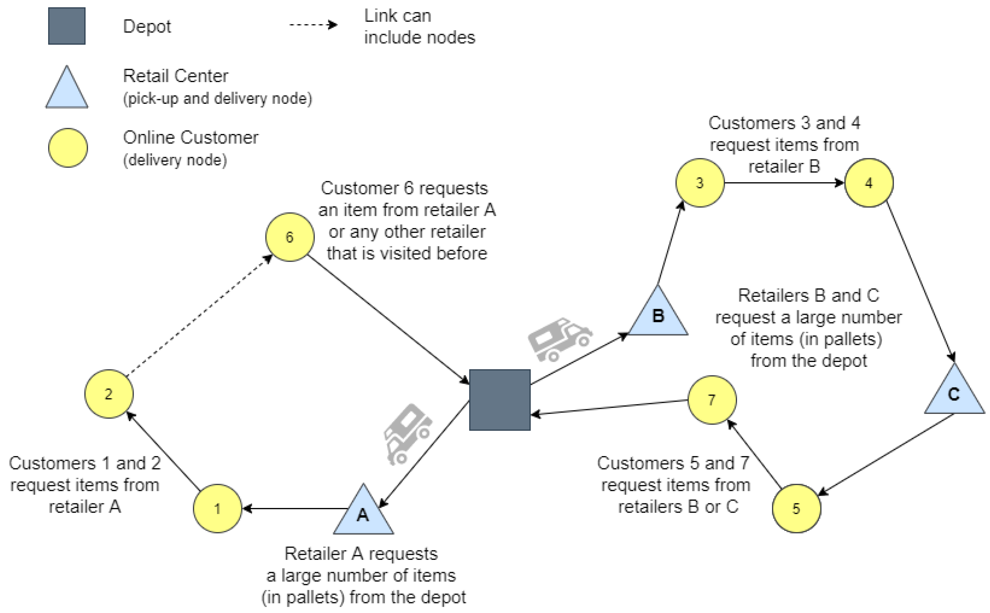
Figure 1 depicts how the processes of visiting retail centers and online customers are performed by the same fleet of vehicles. A route starts from the single and central depot, and the same cargo vehicle visits a set of retail centers and customers. Deliveries to customers cannot be directly performed from the depot. Hence, drivers must meet precedence constraints in order to pick-up customer orders from the retail centers before they can be delivered. Since retailers are supplied by the depot, these nodes are both delivery and pick-up points. On the other hand, customers require only the delivery of items from these retail centers, making them, delivery nodes. Apart from precedence and inventory constraints, the service of each route is limited by a maximum tour length and vehicle capacity limit.
We can define the distribution network of the OM-VRP as directed graph G = ( V , A ) . The set of vertices V = { 0 , 1 , 2 , , r + c } is composed of a single depot (0), r retail centers, and c online customers. In other words, the problem is represented by a set R of retail stores, which are supplied by the depot 0, and a set C of online customers, which are posteriorly supplied by the retail centers. The set N = R C comprises both sets R and C, in which R = { 1 , 2 , , r } and C = { r + 1 , r + 2 , , r + c } . The same fleet of capacitated vehicles, initially stationed at the central depot at the start time t 0 , is employed for serving both the retail centers and consumers. For the complete mathematical formulation of this problem, readers are referred to Abdulkader et al. [1]. In this work, we extend previous work on this topic by considering the case in which edge-traversal times are stochastic. We define the time to traverse edge ( i , j ) as T i j = t i j + D i j where t i j is the deterministic edge-traversal time (which represents the edge-traversal time under ‘ideal’ traffic conditions), D i j is a log-normally distributed delay term, and T i j denotes the distribution of edge-traversal times. The objective of this extended problem is to minimize the total travel cost of the vehicle routes such that: (i) every route starts and ends at the depot; (ii) the routes do not violate the maximum tour length; (iii) every node i N is visited by only one vehicle and only once; (iv) the total load of the vehicle does not exceed the vehicle capacity; (v) the total consumer demand to be fulfilled by a vehicle for a specific product does not exceed the inventory picked up by the vehicle; (vi) the retail store determined to satisfy the consumer’s demand must be visited before the consumer and by the same vehicle; and (vii) the routes must have a reliability level greater than a user-set parameter, R m i n . The reliability level of a set of routes is defined as the probability that all routes are completed within the maximum time limit of T m a x .
Two alternative mathematical formulations of the deterministic OM-VRP can be found in Abdulkader et al. [1], Bayliss et al. [37]. The differences in this case are a stochastic objective function and probabilistic constraint regarding route completion reliability. Let x f k i j be a binary decision variable indicating whether or not vehicle f in the fleet F traverses edge i j in the k t h node visit in its route. The stochastic objective function is given in Equation (1), where D i j is the stochastic delay associated with traversing edge i j .
m i n E f F k K i V j V x f k i j t i j + D i j .
The probabilistic route completion reliability constraint is given in Equation (2).
R m i n P i V j N k K t i j + τ + D i j x f k i j + i V k K t i 0 + D i 0 x f k i 0 T m a x , f F .
Equation (2) also accounts for the drop times ( τ ) that are required when performing deliveries and pickups. In this work we employ a simheuristic approach for addressing the stochastic aspects of the OM-VRP. The main novelty of the OM-VRP, in comparison to other VRPs, is the precedence constraints regarding the collection of customer orders from retailers and subsequent delivery to customers. The vehicle capacity constraint regarding the retailer demands that can be satisfied are expressed by Equation (3), where O P j denotes the number of ordered product units of node j (which is zero for customer nodes) and H denotes the vehicle capacity.
i N j V l = 1 k x f l i j O P j H , f F , k K .
The customer order precedence constraints are expressed by Equation (4), where O D j q denotes the number of items of type q Q ordered by node j (which is zero for retailer nodes) and P j q denotes the number of items picked up of type q Q at node j (which is zero for customer nodes).
i V j V l = 1 k x f l i j P j q O D j q 0 , f F , k K , q Q .
Table 1 provides the details for a small-sized instance, which is composed of one central warehouse, four retail stores, and nine online customers. For this instance, Table 1 provides: the geographic coordinates (X and Y) of each node, the demand required from the depot by each retail center i R , the demands for each customer j for each product type q ( O D j q ), and the inventory of each available product P i q , q { 1 , 2 , 3 } at the retail centers. Since the products are negligible in terms of capacity, they do not affect the vehicle load capacity. Accordingly, Figure 2 presents the optimal solution for the provided example. The routes are performed with a total cost of 455.91 distance units, and a fleet of vehicles each with a capacity of 100 weight units is employed for performing the routes. In the first route, customers 8, 5, and 9 are served by retail center 1, while customers 12 and 13 are served by retail 3. The route requires 272.37 distance units, and the vehicle starts with 93 loaded demand units. Note that the retail centers are first visited by the vehicle in order to deliver the required demand from the depot and to pick-up the products ordered by the customers. Similarly, in the second route, customers 11 and 10 are supplied by retail center 4 while customers 6 and 7 are served by retail store 2. The route requires 183.53 distance units, starting with 79 loaded demand units.

4. Methodology

The multi-start framework belongs to a family of metaheuristics algorithms [56] which includes approaches such as Evolutionary Algorithms [57,58] and Swarm Intelligence Algorithms [59,60,61,62], among others. Metaheuristics were introduced in order to provide high-quality solutions using a reasonable amount of computation time and memory. Typically, they require a time-consuming parameter tuning process. Although, there are approaches that provide self-adaptive parameter control [58], our methodology has been devised to work with a reduced number of parameters, providing an excellent trade-off between simplicity, computational time, and solution quality.
In order to solve the stochastic OM-VRP, a simheuristic approach is proposed. Our methodology combines a biased-randomized savings-based heuristic with simulation techniques to deal with the stochastic aspects of the problem. Biased-randomized heuristics can be extended into simheuristics in a natural way. Starting from a savings-based heuristic, which is completely deterministic, this solution method is then extended into a biased-randomized multi-start algorithm. Also, a local search procedure is applied to search for locally optimal solutions. Finally, the multi-start framework is extended into a simheuristic approach in order to deal with stochastic travel times.

4.1. Savings-Based Heuristic

As introduced, the savings-based heuristic (LH) [9] is based on greedy decisions and designed to solve the deterministic OM-VRP. The LH is composed of the following three stages:
  • In the first stage, a dummy solution is created, where each route in this dummy solution serves one node i N , which can be either a consumer or a retail store. Routes depart from the depot, travel to the node, and then return to the depot.
  • The second stage of LH, named as CWS 1 , is presented in the Figure 3, where the dummy routes from stage 1 are merged using a maximum-savings criterion [36]. Each box from Figure 3 is numbered to aid the following explanations.
    Initially, a savings list (SL) is constructed (step 1). This list considers all possible pairs of nodes–i.e., edges–from the problem. For each edge { i , j } , the corresponding savings value is calculated as s i j = t 0 i + t j 0 t i j , where t i j represents the deterministic travel time between nodes i and j. That is, candidate solutions are generated using ‘ideal’ traffic conditions for the edge-traversal times.
    Initially, all edges from SL are eligible. The list is sorted in descending order of the savings value (step 2), and the edge with the highest saving is selected (step 3). At this stage, the selection of edges is restricted to guarantee the assignment of a retail center to each consumer in the problem (step 5). In other words: a route containing one single customer can only be merged with a route containing a retail center, i.e., the selection is restricted to eligible edges { i , j } , where node j is a consumer in a dummy route and i is a node in a route with a retailer that can supply consumer j. According to Martins et al. [9], these attempts at only merging routes containing at least one retail center, which can supply a single consumer, are made first in order to avoid infeasible solutions–i.e., solutions in which some customers are not assigned to any retailer. This approach of addressing solution feasibility first is based on the observation that the availability of feasibility restoring merges will only decrease as the algorithm progresses.
    Based on CWS route-merging conditions (step 6), the two corresponding routes, i and j, of an edge { i , j } (obtained in steps 4.1 and 4.2 ) can be merged only if: (i) nodes i and j are exterior in their respective routes (a node is exterior if it is adjacent to the depot); (ii) i and j belong to different routes; (iii) the maximum tour length is not violated; and (iv) the vehicle capacity is not violated.
    The selected edge is deleted from SL (step 9) only if: (a) the corresponding merge is performed (step 7); or (b) at least one of the CWS constraints ((i)–(iv)) are violated (in step 6). Otherwise, the edge becomes temporarily ineligible (step 10), but it is not removed from the list since subsequent merges might restore eligibility. This can occur when a different retail center is merged into a route, increasing the available processed inventory for subsequent consumers. For example, when selecting an edge ( i , j ) , the evolving route of i may have insufficient processed inventory for customer j at this time. However, if in subsequent iterations route i is merged with another route containing retailers, the evolving route of i may then be able to serve customer j.
    When a merge is successfully performed (step 7), the entire SL becomes eligible (step 8), since a new inventory scenario is generated.
    At the end of this stage, all the consumers are supplied by the retail centers, guaranteeing a feasible final solution. Notice that this is achieved without solving separate assignment and routing problems, as done in Abdulkader et al. [1].
  • Finally, the third stage (CWS 2 ) tries to improve the solution generated in the previous step. To do that, the algorithm cycles through the SL list, which includes the remaining saving edges that were discarded in the previous step, with the aim of identifying more beneficial merges. Unlike the procedure used in the CWS 1 stage, in this phase all the customers are already assigned to a retail center, so step 5 of Figure 3 is not required. Hence, all edges are eligible. The process attempts all the available merging possibilities which may improve the solution. Each time a new edge is selected from the SL list, it is removed from the list, whether the corresponding merge is performed or not–due to it violating any of the constraints (i)–(iv). In each new iteration, the highest saving edge is selected to restart the merge process. This process is repeated until SL is empty. At the end of the procedure, a feasible solution is generated, without the necessity of repair operations.

4.2. Introducing a Local Search

Once an initial and feasible solution is constructed, a fast local search is applied to improve its quality. This local search mechanism is based on a 2-opt movement. Since this problem has some precedence particularities, the 2-opt movement, which consists of the reversal of sub-sequence of nodes, is restricted to movements that do not violate the precedence order between customers and their suppliers–hence, the feasibility of the solution is preserved.

4.3. Extending to a Biased-Randomized Algorithm

To modify the original greedy and deterministic behavior of our heuristic, the selection of candidates from the SL is randomized by introducing a skewed probability distribution into the selection process. For the biased-randomized component, we employ a geometric distribution, which is controlled by a single parameter, β ( 0 , 1 ) . β values closer to 1 increase the probability that the highest saving merges are selected. On the contrary, as β approaches 0, a near-uniform randomization is obtained. In this way, β controls the level at which the selection probabilities decrease along the sorted SL. Hence, unlike deterministic heuristics, which always generate the same solution when starting from the same initial solution, different decisions are taken at each selection iteration, consequently generating different solutions. Algorithm 1 represents the selection process of LH with biased-randomization, which replaces the greedy selection of edges from the SL.
Algorithm 1: brSelection.
Data: savings list S L , parameter β 0 , 1
1 l getNumberOfEligibleEdgesFromList ( S L );
2 Randomly select position x { 1 , , l } according to distribution Geom ( β );
3 e selectTheXthEligibleEdgeFromList ( x , S L );
4returne;
Considering all of the stages which have been introduced, Algorithm 2 represents the overall structure of our biased-randomized algorithm with local search (BRLH). This algorithm is then embedded into a multi-start procedure in order to obtain a variety of solutions (MSBRLH).
Algorithm 2: BRLH.
Data: set of nodes V, geometric distribution parameter β
1 s o l createDummySolution (V);
2 s o l CWS 1  ( s o l , β );
3 s o l CWS 2  ( s o l , β );
4 s o l localSearch ( s o l );
5return s o l

4.4. Extending to a Simheuristic Approach

Deterministic travel times are widely assumed in transportation problems. However, when dealing with real-life problems, which are often fraught with uncertainty, travel times are usually stochastic in nature. As introduced in Section 3, the deterministic travel time employed to traverse edge ( i , j ) , t i j , can be seen as the travel time required under ideal traffic conditions. In the proposed extension, the stochastic time to traverse ( i , j ) is computed as T i j = t i j + D i j , where D i j follows a l o g N o r m a l ( μ , σ ) probability distribution, and represents a random delay resulting from uncertain conditions. Since the l o g N o r m a l probability distribution can only take positive values, it follows that T i j > t i j , ( i , j ) in the set of connecting edges.
Algorithm 3 describes our simheuristic approach (SimBRLH). Initially, a solution is generated by our BRLH in line 1 (Algorithm 2), by employing the greedy approach (i.e., β 1 ). A short simulation is then performed on this initial solution (line 2), in order to estimate its average stochastic cost. This initial solution is set as the best-found stochastic solution cost (line 4). While the termination criterion is not met (line 6), different solutions are generated by BRLH (line 7). The deterministic cost of the initial solution is considered for guiding the search. Therefore, a solution is accepted for being submitted to the simulation module (line 10) only if its deterministic cost is smaller than the best-found deterministic solution cost plus m % of its value (line 9). This solution filtering approach reduces the amount of time spent on testing unpromising solutions in computationally expensive simulations. Moreover, by allowing the acceptance of moderately worse solutions, controlled by the parameter m, a better exploration of the solution space can be achieved [63]. At this stage, q s h o r t Monte Carlo simulation runs are used to test the accepted solution. Each simulation run replaces the deterministic travel times of a solution with randomly sampled ones–according to the assumed probability distribution. From this complete simulation process, the average stochastic cost of each solution is computed. Every time a new best stochastic cost is found (line 15), this solution is introduced into a pool of ‘elite’ solutions E (line 17). This process is repeated while the termination criterion is not met. On this reduced set of solutions, q l o n g Monte Carlo simulation runs are performed (line 23) in order to generate more accurate results for solutions in stochastic environments. During the simulation process we also obtain an estimate of the reliability rate of a solution [64]. This estimate is computed as the rate at which all routes show completion times lower than the maximum allowed travel time. At the end, the set of elite solutions is sorted in descending order of their expected cost (line 25), and the best-found stochastic solution is provided to the manager.
Algorithm 3: SimBRLH.
Algorithms 13 00237 i001

5. Results and Discussion

To test the proposed methodologies, we have used the 60 problem instances introduced in Abdulkader et al. [1]. These instances differ in the number of retail centers ( r { 10 , 15 , 20 , 25 } ), online customers ( c { 20 , 50 , 75 , 100 , 150 } ), and also in the inventory scenarios of the retail centers (tight, relaxed, and abundant). Therefore, for each inventory scenario, 20 different problem combinations are generated. The maximum tour length of the routes and the vehicle capacity are set to 8 h and 100 weight units, respectively. While the BRLH is guided by a single parameter, β , the simheuristic approach is also controlled by the maximum running time t i m e m a x , the acceptance margin of worst solutions m, and the number, q s h o r t and q l o n g , of simulation repeats in short and long simulation runs, respectively. The stochastic travel times for each edge are set by the log-normal distribution parameters, μ and σ .
Table 2 summarizes the setup of the parameters employed during the computational experiments. For calibrating these parameters, we have used the methodology proposed in Calvet et al. [65], which is based on a general and automated statistical learning procedure. Regarding the maximum run time t i m e m a x , the value was set depending on the size of the instance ( c + r ) × 0.342 , which leads to a maximum execution time of 60 s in the case of the largest instance. This stopping criterion is employed in both the multi-start and simheuristic strategies.
The algorithms were coded in Java and all tests were performed on an Intel Core i7-8550U processor with 16 GB of RAM.
Note that three different values have been considered for the σ parameter, which is used to modify the deterministic travel times. Since the maximum tour length is fixed independently of the size of the instances, small-sized instances are more likely to generate short routes. Therefore, a larger value for σ introduces more variability in the travel times, which increases route failure rates. On the other hand, large-sized instances are often composed of larger routes, then a small value for σ is introduced. In particular we have, σ = 2.5 for small instances (composed of 25 customers), σ = 1.55 for large instances (composed of 150 customers), and σ = 1.9 for the remaining medium-sized ones. This approach ensures that small, medium, and large instances each have similar levels of difficulty with respect to the risk of route failure.
The initial analysis aims to compare the solutions generated by our greedy heuristic (LH) and by our MSBRLH–in which β is (uniformly) randomly selected in the interval [ 0.45 , 0.75 ] –with the solutions obtained by the two-phase heuristic (AH) and multi-ant colony metaheuristic (MAC) proposed by Abdulkader et al. [1]. Their methodologies were performed on four 2.1 GHz processors with 16-cores each and a total of 256 GB RAM. That is, we initially focus on comparing each algorithm in terms of deterministic travel cost. Table 3, Table 4 and Table 5 present the results obtained for tight, relaxed, and abundant inventory scenarios, respectively. For each problem instance (I), we present results for: the cost of the best-found solution obtained by the different methodologies; the average cost of our MSBRLH; the CPU time (in seconds) required by each methodology; and their percentage gaps. The best results returned by the solution methodologies are highlighted in bold. Figure 4 and Figure 5 present how both the gap and the cost of the solutions, i.e., the objective function (OF) value, behave according to the employed solution approach and inventory scenario, respectively.
By analyzing Table 3, Table 4 and Table 5, we can observe that our MSBRLH algorithm is able to improve previous results (from LH) by 9–12%, on average (column gap (2)–(1)). When comparing the MSBRLH with the AH heuristic (column gap (3)–(2)), our approach is able to reduce solution costs by up to 26% in short computational times (about 18 s on average). On the other hand, when comparing our results with those generated by the MAC approach (column gap (4)–(2)), our solutions are between 9% and 21% worse, on average. Particularly, in the abundant inventory scenario, MSBRLH’s results are only 9% worse than MAC. Notice, however, that the processing time required by MAC is substantially larger in all inventory scenarios. By analyzing 
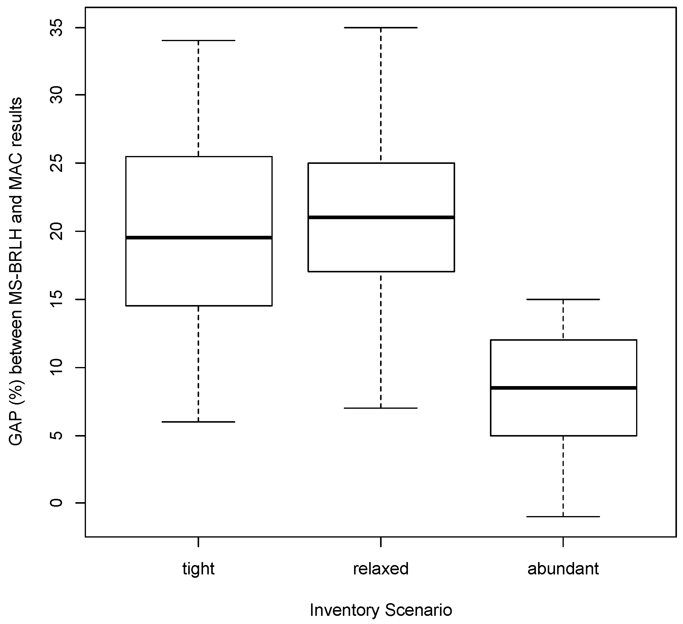
Figure 4, it is evident that MSBRLH performs better in the abundant inventory scenario, being able to find one better solution and several others with a maximum gap of 8%. Moreover, we can observe a variability of around 10% in the gap between MSBRLH and MAC on average. This variability is reduced to around 8% for the relaxed and abundant scenarios. These results demonstrate the robustness of our solution approach for the deterministic case. When analyzing 
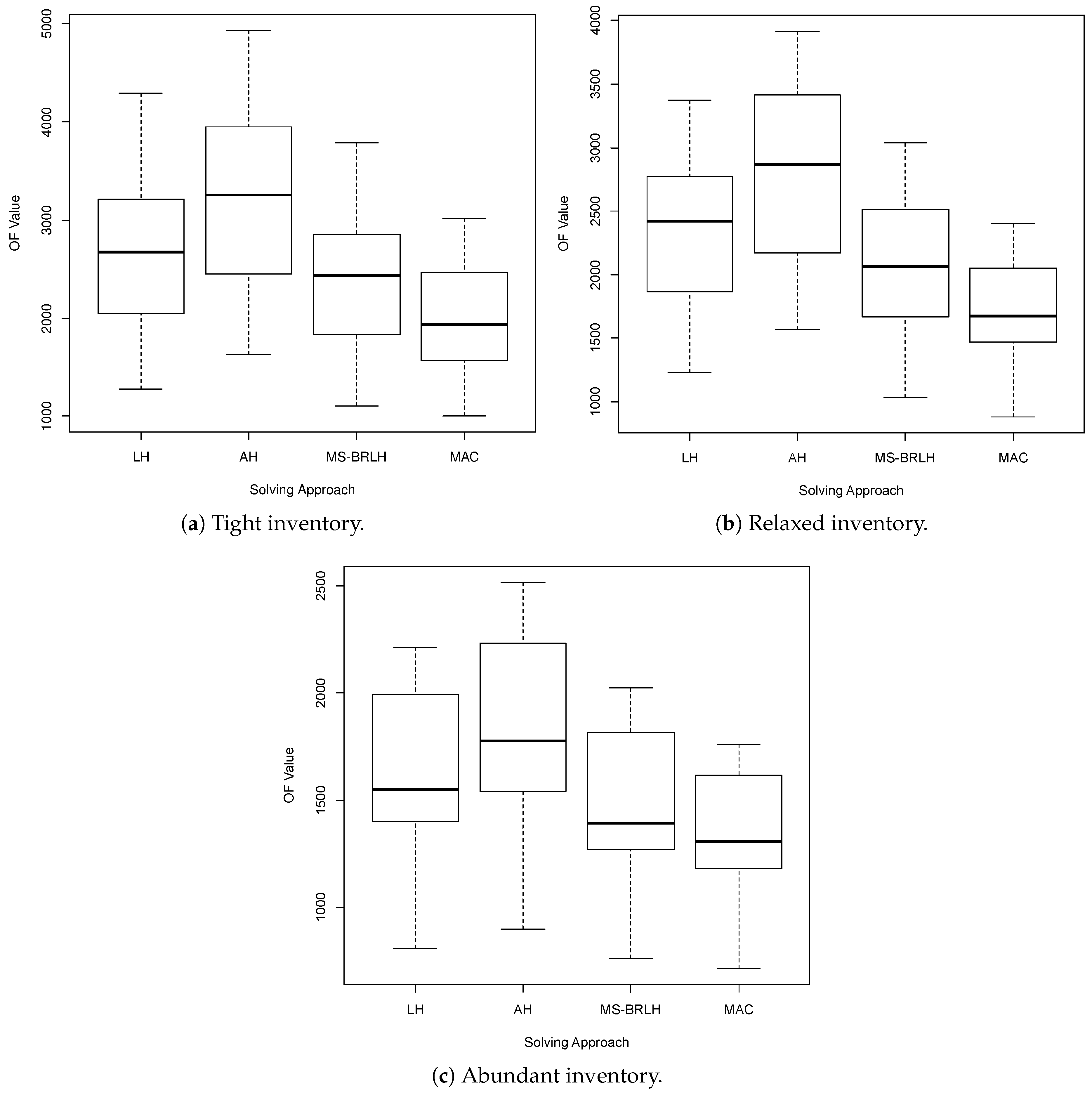
Figure 5, which presents the overall performance of each solution approach for each inventory scenario, we can observe that our multi-start strategy is more efficient than both LH and AH heuristics, by generating solutions with a lower cost. To complement these box-plots, an ANOVA test was run for each inventory scenario. The p-values associated with the tight, relaxed, and abundant inventory scenarios were, respectively, of 0.001 , 0.000 , and 0.000 . Also, the Fisher’s LSD test suggests significant differences in all tree scenarios between MAC and AH, between MS-BRLH and AH, as well as between MAC and LH. However, cost differences between MAC and MS-BRLH were not significant in any scenario, despite the fact that MAC employed a noticeably higher amount of computing time than MS-BRLH.
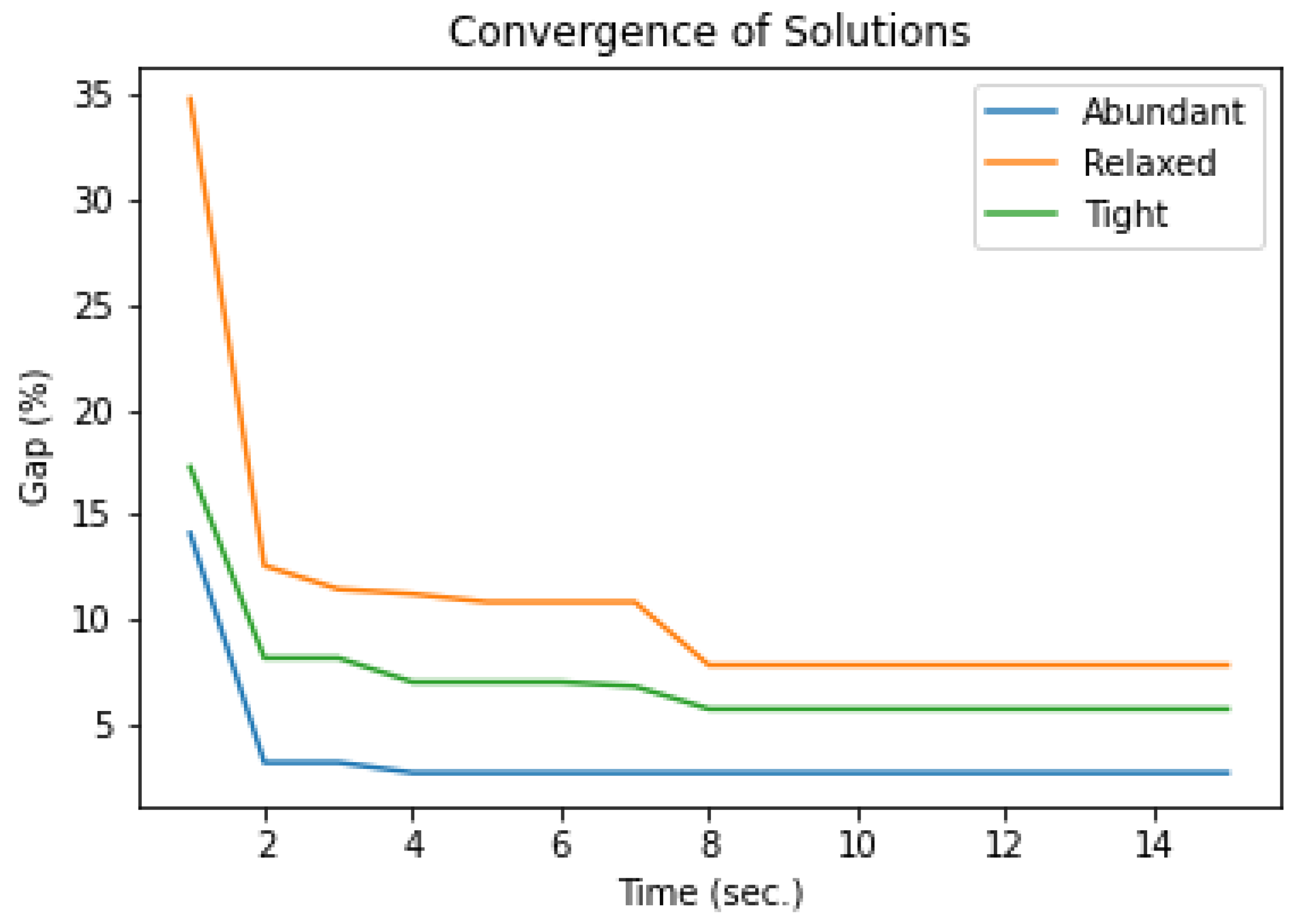
Next, in Figure 6, we present the convergence of three problem instances’ solutions, including one from each different inventory scenario (instances b 6 , b 26 , and b 46 ), by comparing the MSBRLH with the best-known solutions, in terms of gap. As introduced, these instances require approximately 15 s of processing time, given their magnitude.
As we can see in Figure 6, the instances demonstrate the same convergence behavior as solution time increases. It is noticeable that the convergence rate is abrupt during the first few seconds. However, contrary to the tight and relaxed inventory scenarios, where the solutions continue improving over time, the search demonstrates more stable convergence during the remaining execution time in the abundant scenario. Being more efficient in the more flexible inventory case, our multi-start approach quickly achieves its best solutions.
Next, we want to compare the quality of the solutions generated for the deterministic scenario (MSBRLH) against the solutions generated for the stochastic scenario (SimBRLH). Since the only difference between the deterministic and stochastic scenarios is that stochastic delays are added to edge traversal times, we can consider the deterministic cost of the best solutions generated by MSBRLH as a lower bound (LB) of the stochastic travel times of the best SimBRLH solution. Moreover, since MSBRLH does not account for stochastic travel times, we can consider the stochastic travel time of the best MSBRLH solution as an upper bound (UB) for the stochastic travel time of the best SimBRLH solutions. Table 6 provides both LBs and UBs values and the best-found stochastic travel times obtained by our SimBRLH. The solutions reported in the SimBRLH column are the best-found stochastic travel times.
As we can see in Table 6, all the SimBRLH solution costs are between the LB and the UB, as expected. For 24 problem instances, the solution returned by our simheuristic is better than the best deterministic solution when it is tested in the stochastic scenario (the U B column). From this, we can assert that our Sim
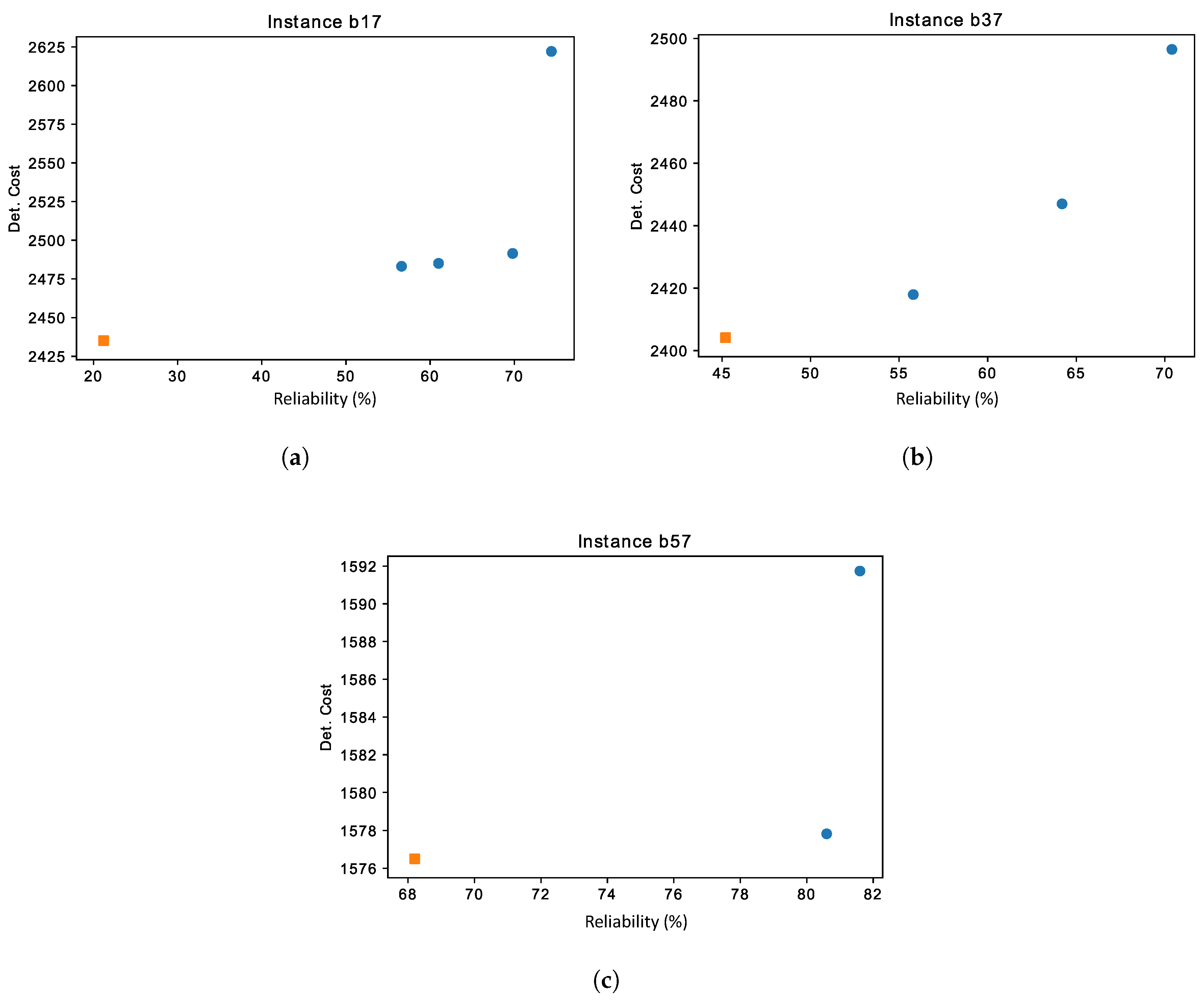
BRLH is able to generate competitive results for the stochastic scenario. The reliability value is calculated by simulation for each solution and represents the probability that all routes are completed within maximum tour duration. For visualizing this trade-off between the deterministic cost of the solutions and their reliability rate, which are conflicting objectives, a Pareto frontier of non-dominated is presented. Accordingly, Figure 7a–c present the non-dominated solutions for three different instances ( b 17 , b 37 , and b 57 ), each one belonging to a different inventory scenario. A solution is non-dominated if, no other solution has a greater reliability and a lower or equal travel cost, or if no other solution has a lower travel cost and a greater or equal reliability level. The b 17 solution was randomly chosen, while the b 37 and b 57 solutions are for the same problem but set in the two other inventory scenarios. The square orange dot represents the best deterministic solution found by our MSBRLH, while the remaining ones, round and blue, represent different solutions with a higher reliability rate, but with higher operating costs.
As we can see in Figure 7, despite being the solutions with the lowest cost, the best deterministic solutions (square dots) are the least reliable ones for stochastic scenarios. Particularly in Figure 7a, the best deterministic solution is approximately only 21% reliable under stochasticity. By selecting higher-cost solutions, the reliability rate reaches more than 70%. The same behavior is noticed in Figure 7b,c, however, the deterministic b 57 solution is reasonably reliable. Usually, low-cost solutions are made up of a small number of large vehicle routes, in terms of travel distance and time. Therefore, when increasing the travel time variability in those scenarios, the risk of exceeding the time constraint is higher. On the other hand, higher cost solutions are built from a larger number of smaller routes, and smaller routes exhibit a lower risk of violating the maximum tour duration constraint in stochastic scenarios. In this way, decision-makers should consider that low-cost solutions under deterministic scenarios might not necessarily be the best option when stochasticity is taken into account.

6. Conclusions and Future Work

With the emergence of online retail channels and the popularization of mobile devices, new retailing modes have become popular. Some of these retailing practices allow customers to browse through different online stores and, then, to get the items bought directly delivered to their homes. Hence, new versions of the vehicle routing problem (VRP) considering additional decision variables and constraints have emerged. Omnichannel retailing leads to an integrated problem combining the VRP and the pick-up and delivery problem. In omnichannel distribution systems, a set of retail stores need to be replenished and, at the same time, products have to be sent from these stores to final customers. The resulting omnichannel VRP consists in two stages: (i) a group of retail stores that must be served from a distribution center; and (ii) a set of online consumers who must be served, by the same fleet of cargo vehicles, from these retail stores.
For solving the deterministic OM-VRP, a simple heuristic was initially introduced. This heuristic was then extended into a multi-start biased-randomized algorithm, which is tested against the state-of-the-art methodologies. Our biased-randomized algorithm performs reasonably well in a set of 60 instances of the deterministic OM-VRP, which allows us to extend it into a full simheuristic for solving the stochastic version of the problem. This is a more realistic version of the OM-VRP where travel times are modeled as random variables following a log-normal distribution. Our simheuristic approach is also capable of measuring the reliability of any proposed solution when it is employed in a stochastic scenario. To the best of our knowledge, this is the first time that such a stochastic variant of the problem has been solved in the literature. Regarding the simheuristic results, we conclude that the best deterministic solutions may perform badly when used in a stochastic scenario. Those solutions are often not reliable in terms of completing all routes within a time limit. On the other hand, our simheuristic approach was able to generate reliable and competitive results for these stochastic scenarios. Therefore, our methodology enables decision makers to choose the solution that better fits his or her utility function in terms of cost and reliability level.
Two-echelon distribution systems, as the one considered here, are typically characterized by the use of different fleets of vehicles at each distribution level. Apart from considering a single fleet of vehicles for serving both delivery levels, the products ordered by customers were assumed to not affect the vehicles’ capacity. Therefore, future directions of research include the consideration of non-negligible sized online customer orders, heterogeneous vehicle fleets, and the incorporation of positive demands for multiple product types for each customer. Regarding the solution approach, different perturbation stages and local search operators could be tested in order to speed up the convergence process towards near-optimal solutions. This might be particularly relevant when considering large-sized instances.

Author Contributions

Conceptualization, L.d.C.M., C.B. and A.A.J.; methodology, L.d.C.M., C.B., P.J.C.-M., J.P. and A.A.J.; software, L.d.C.M. and P.J.C.-M.; writing, L.d.C.M., C.B., P.J.C.-M., J.P. and A.A.J.; validation, L.d.C.M., P.J.C.-M., J.P. and A.A.J. All authors have read and agreed to the published version of the manuscript.

Funding

This research received no external funding.

Acknowledgments

This work has been partially supported by Rhenus Freight Logistics GmbH & Co. KG and by the Spanish Ministry of Science, Innovation, and Universities (PID2019-111100RB-C21, RED2018-102642-T). We also acknowledge the support of the Erasmus+ Program (2019-I-ES01-KA103-062602).

Conflicts of Interest

The authors declare no conflict of interest.

References

  1. Abdulkader, M.M.S.; Gajpal, Y.; ElMekkawy, T.Y. Vehicle routing problem in omni-channel retailing distribution systems. Int. J. Prod. Econ. 2018, 196, 43–55. [Google Scholar] [CrossRef]
  2. Gallino, S.; Moreno, A. Integration of online and offline channels in retail: The impact of sharing reliable inventory availability information. Manag. Sci. 2014, 60, 1434–1451. [Google Scholar] [CrossRef] [Green Version]
  3. Hübner, A.; Holzapfel, A.; Kuhn, H. Distribution systems in omni-channel retailing. Bus. Res. 2016, 9, 255–296. [Google Scholar] [CrossRef] [Green Version]
  4. Quintero-Araujo, C.L.; Gruler, A.; Juan, A.A.; Faulin, J. Using horizontal cooperation concepts in integrated routing and facility-location decisions. Int. Trans. Oper. Res. 2019, 26, 551–576. [Google Scholar] [CrossRef]
  5. Crainic, T.G.; Laporte, G. Fleet Management and Logistics; Springer Science & Business Media: Berlin/Heidelberg, Germany, 2012. [Google Scholar]
  6. Cheng, B.Y.; Leung, J.Y.T.; Li, K. Integrated scheduling of production and distribution to minimize total cost using an improved ant colony optimization method. Comput. Ind. Eng. 2015, 83, 217–225. [Google Scholar] [CrossRef]
  7. Lenstra, J.K.; Kan, A. Complexity of vehicle routing and scheduling problems. Networks 1981, 11, 221–227. [Google Scholar] [CrossRef] [Green Version]
  8. Savelsbergh, M.W.; Sol, M. The general pickup and delivery problem. Transp. Sci. 1995, 29, 17–29. [Google Scholar] [CrossRef] [Green Version]
  9. Martins, L.D.C.; Bayliss, C.; Juan, A.A.; Panadero, J.; Marmol, M. A savings-based heuristic for solving the omnichannel vehicle routing problem with pick-up and delivery. Transp. Res. Procedia 2020, 47, 83–90. [Google Scholar] [CrossRef]
  10. Quintero-Araujo, C.L.; Caballero-Villalobos, J.P.; Juan, A.A.; Montoya-Torres, J.R. A biased-randomized metaheuristic for the capacitated location routing problem. Int. Trans. Oper. Res. 2017, 24, 1079–1098. [Google Scholar] [CrossRef]
  11. Juan, A.A.; Kelton, W.D.; Currie, C.S.; Faulin, J. Simheuristics applications: Dealing with uncertainty in logistics, transportation, and other supply chain areas. In Proceedings of the 2018 Winter Simulation Conference, Gothenburg, Sweden, 9–12 December 2018; pp. 3048–3059. [Google Scholar]
  12. Gonzalez-Martin, S.; Juan, A.A.; Riera, D.; Elizondo, M.G.; Ramos, J.J. A simheuristic algorithm for solving the arc routing problem with stochastic demands. J. Simul. 2018, 12, 53–66. [Google Scholar] [CrossRef]
  13. Gruler, A.; Fikar, C.; Juan, A.A.; Hirsch, P.; Contreras-Bolton, C. Supporting multi-depot and stochastic waste collection management in clustered urban areas via simulation–optimization. J. Simul. 2017, 11, 11–19. [Google Scholar] [CrossRef]
  14. Mosquera, A.; Pascual, C.O.; Ayensa, E.J. Understanding the customer experience in the age of omni-channel shopping. Icono14 2017, 15, 5. [Google Scholar] [CrossRef] [Green Version]
  15. Verhoef, P.C.; Kannan, P.K.; Inman, J.J. From multi-channel retailing to omni-channel retailing: Introduction to the special issue on multi-channel retailing. J. Retail. 2015, 91, 174–181. [Google Scholar] [CrossRef]
  16. Hübner, A.; Wollenburg, J.; Holzapfel, A. Retail logistics in the transition from multi-channel to omni-channel. Int. J. Phys. Distrib. Logist. Manag. 2016, 46, 562–583. [Google Scholar] [CrossRef]
  17. Heitz-Spahn, S. Cross-channel free-riding consumer behavior in a multichannel environment: An investigation of shopping motives, sociodemographics and product categories. J. Retail. Consum. Serv. 2013, 20, 570–578. [Google Scholar] [CrossRef]
  18. Beck, N.; Rygl, D. Categorization of multiple channel retailing in Multi-, Cross-, and Omni-Channel Retailing for retailers and retailing. J. Retail. Consum. Serv. 2015, 27, 170–178. [Google Scholar] [CrossRef]
  19. Dantzig, G.B.; Ramser, J.H. The truck dispatching problem. Manag. Sci. 1959, 6, 80–91. [Google Scholar] [CrossRef]
  20. Laporte, G.; Mercure, H.; Nobert, Y. An exact algorithm for the asymmetrical capacitated vehicle routing problem. Networks 1986, 16, 33–46. [Google Scholar] [CrossRef]
  21. Fukasawa, R.; Longo, H.; Lysgaard, J.; de Aragão, M.P.; Reis, M.; Uchoa, E.; Werneck, R.F. Robust branch-and-cut-and-price for the capacitated vehicle routing problem. Math. Program. 2006, 106, 491–511. [Google Scholar]
  22. Barbarosoglu, G.; Ozgur, D. A tabu search algorithm for the vehicle routing problem. Comput. Oper. Res. 1999, 26, 255–270. [Google Scholar]
  23. Nazif, H.; Lee, L.S. Optimised crossover genetic algorithm for capacitated vehicle routing problem. Appl. Math. Model. 2012, 36, 2110–2117. [Google Scholar] [CrossRef]
  24. Ezzatneshan, A. A algorithm for the Vehicle Problem. Int. J. Adv. Robot. Syst. 2010, 7, 14. [Google Scholar] [CrossRef]
  25. Lin, S.W.; Lee, Z.J.; Ying, K.C.; Lee, C.Y. Applying hybrid meta-heuristics for capacitated vehicle routing problem. Expert Syst. Appl. 2009, 36, 1505–1512. [Google Scholar] [CrossRef]
  26. Lu, Q.; Dessouky, M. An exact algorithm for the multiple vehicle pickup and delivery problem. Transp. Sci. 2004, 38, 503–514. [Google Scholar] [CrossRef]
  27. Ropke, S.; Cordeau, J.F. Branch and cut and price for the pickup and delivery problem with time windows. Transp. Sci. 2009, 43, 267–286. [Google Scholar] [CrossRef] [Green Version]
  28. Nanry, W.P.; Barnes, J.W. Solving the pickup and delivery problem with time windows using reactive tabu search. Transp. Res. Part B Methodol. 2000, 34, 107–121. [Google Scholar] [CrossRef]
  29. Pankratz, G. A grouping genetic algorithm for the pickup and delivery problem with time windows. OR Spectr. 2005, 27, 21–41. [Google Scholar] [CrossRef] [Green Version]
  30. Ropke, S.; Pisinger, D. An adaptive large neighborhood search heuristic for the pickup and delivery problem with time windows. Transp. Sci. 2006, 40, 455–472. [Google Scholar] [CrossRef]
  31. Li, Y.; Chen, H.; Prins, C. Adaptive large neighborhood search for the pickup and delivery problem with time windows, profits, and reserved requests. Eur. J. Oper. Res. 2016, 252, 27–38. [Google Scholar] [CrossRef]
  32. Ghilas, V.; Demir, E.; Van Woensel, T. An adaptive large neighborhood search heuristic for the pickup and delivery problem with time windows and scheduled lines. Comput. Oper. Res. 2016, 72, 12–30. [Google Scholar] [CrossRef] [Green Version]
  33. Ai, T.J.; Kachitvichyanukul, V. A particle swarm optimization for the vehicle routing problem with simultaneous pickup and delivery. Comput. Oper. Res. 2009, 36, 1693–1702. [Google Scholar] [CrossRef]
  34. Nadizadeh, A.; Kafash, B. Fuzzy capacitated location-routing problem with simultaneous pickup and delivery demands. Transp. Lett. 2019, 11, 1–19. [Google Scholar] [CrossRef]
  35. Berbeglia, G.; Cordeau, J.F.; Gribkovskaia, I.; Laporte, G. Static pickup and delivery problems: A classification scheme and survey. Top 2007, 15, 1–31. [Google Scholar] [CrossRef]
  36. Clarke, G.; Wright, J.W. Scheduling of vehicles from a central depot to a number of delivery points. Oper. Res. 1964, 12, 568–581. [Google Scholar] [CrossRef]
  37. Bayliss, C.; Martins, L.D.C.; Juan, A.A. A Two-phase Local Search with a Discrete-event Heuristic for the Omnichannel Vehicle Routing Problem. Comput. Ind. Eng. 2020, 148, 106695. [Google Scholar] [CrossRef]
  38. Martins, L.D.C.; Hirsch, P.; Juan, A.A. Agile optimization of a two-echelon vehicle routing problem with pickup and delivery. Int. Trans. Oper. Res. 2020, 28, 201–221. [Google Scholar] [CrossRef]
  39. Estrada-Moreno, A.; Ferrer, A.; Juan, A.A.; Bagirov, A.; Panadero, J. A biased-randomised algorithm for the capacitated facility location problem with soft constraints. J. Oper. Res. Soc. 2019, 0, 1–17. [Google Scholar] [CrossRef]
  40. Dominguez, O.; Guimarans, D.; Juan, A.A.; de la Nuez, I. A biased-randomised large neighbourhood search for the two-dimensional vehicle routing problem with backhauls. Eur. J. Oper. Res. 2016, 255, 442–462. [Google Scholar] [CrossRef]
  41. Belloso, J.; Juan, A.A.; Faulin, J. An iterative biased-randomized heuristic for the fleet size and mix vehicle-routing problem with backhauls. Int. Trans. Oper. Res. 2019, 26, 289–301. [Google Scholar] [CrossRef] [Green Version]
  42. Dominguez, O.; Juan, A.A.; de La Nuez, I.; Ouelhadj, D. An ILS-biased randomization algorithm for the two-dimensional loading HFVRP with sequential loading and items rotation. J. Oper. Res. Soc. 2016, 67, 37–53. [Google Scholar] [CrossRef] [Green Version]
  43. Al-Behadili, M.; Ouelhadj, D.; Jones, D. Multi-objective biased randomised iterated greedy for robust permutation flow shop scheduling problem under disturbances. J. Oper. Res. Soc. 2019, 1–13. [Google Scholar] [CrossRef]
  44. Ferone, D.; Hatami, S.; González-Neira, E.M.; Juan, A.A.; Festa, P. A biased-randomized iterated local search for the distributed assembly permutation flow-shop problem. Int. Trans. Oper. Res. 2020, 27, 1368–1391. [Google Scholar]
  45. Pages-Bernaus, A.; Ramalhinho, H.; Juan, A.A.; Calvet, L. Designing e-commerce supply chains: A stochastic facility–location approach. Int. Trans. Oper. Res. 2019, 26, 507–528. [Google Scholar]
  46. Rabe, M.; Deininger, M.; Juan, A.A. Speeding up computational times in simheuristics combining genetic algorithms with discrete-Event simulation. Simul. Model. Pract. Theory 2020, 103, 102089. [Google Scholar]
  47. Hatami, S.; Calvet, L.; Fernández-Viagas, V.; Framiñán, J.M.; Juan, A.A. A simheuristic algorithm to set up starting times in the stochastic parallel flowshop problem. Simul. Model. Pract. Theory 2018, 86, 55–71. [Google Scholar]
  48. Gruler, A.; Panadero, J.; de Armas, J.; Moreno, J.A.; Juan, A.A. A variable neighborhood search simheuristic for the multiperiod inventory routing problem with stochastic demands. Int. Trans. Oper. Res. 2020, 27, 314–335. [Google Scholar]
  49. Gruler, A.; Panadero, J.; de Armas, J.; Moreno, J.A.; Juan, A.A. Combining variable neighborhood search with simulation for the inventory routing problem with stochastic demands and stock-outs. Comput. Ind. Eng. 2018, 123, 278–288. [Google Scholar]
  50. Onggo, B.S.; Panadero, J.; Corlu, C.G.; Juan, A.A. Agri-food supply chains with stochastic demands: A multi-period inventory routing problem with perishable products. Simul. Model. Pract. Theory 2019, 97, 101970. [Google Scholar]
  51. Cabrera, G.; Juan, A.A.; Lázaro, D.; Marquès, J.M.; Proskurnia, I. A simulation-optimization approach to deploy Internet services in large-scale systems with user-provided resources. Simulation 2014, 90, 644–659. [Google Scholar]
  52. Panadero, J.; Doering, J.; Kizys, R.; Juan, A.A.; Fito, A. A variable neighborhood search simheuristic for project portfolio selection under uncertainty. J. Heuristics 2020, 26, 353–375. [Google Scholar]
  53. Lam, C.P.; Masek, M.; Kelly, L.; Papasimeon, M.; Benke, L. A simheuristic approach for evolving agent behaviour in the exploration for novel combat tactics. Oper. Res. Perspect. 2019, 6, 100123. [Google Scholar] [CrossRef]
  54. Lopes, T.C.; Michels, A.S.; Lüders, R.; Magatão, L. A simheuristic approach for throughput maximization of asynchronous buffered stochastic mixed-model assembly lines. Comput. Oper. Res. 2020, 115, 104863. [Google Scholar] [CrossRef]
  55. Santos, M.S.; Pinto, T.V.; Júnior, Ê.L.; Cota, L.P.; Souza, M.J.; Euzébio, T.A. Simheuristic-based decision support system for efficiency improvement of an iron ore crusher circuit. Eng. Appl. Artif. Intell. 2020, 94, 103789. [Google Scholar] [CrossRef]
  56. Glover, F.W.; Kochenberger, G.A. Handbook of Metaheuristics; Springer Science & Business Media: Berlin/Heidelberg, Germany, 2006; Volume 57. [Google Scholar]
  57. Dulebenets, M.A.; Moses, R.; Ozguven, E.E.; Vanli, A. Minimizing carbon dioxide emissions due to container handling at marine container terminals via hybrid evolutionary algorithms. IEEE Access 2017, 5, 8131–8147. [Google Scholar] [CrossRef]
  58. Dulebenets, M.A.; Kavoosi, M.; Abioye, O.; Pasha, J. A self-adaptive evolutionary algorithm for the berth scheduling problem: Towards efficient parameter control. Algorithms 2018, 11, 100. [Google Scholar] [CrossRef] [Green Version]
  59. Anandakumar, H.; Umamaheswari, K. A bio-inspired swarm intelligence technique for social aware cognitive radio handovers. Comput. Electr. Eng. 2018, 71, 925–937. [Google Scholar] [CrossRef]
  60. Brezočnik, L.; Fister, I.; Podgorelec, V. Swarm intelligence algorithms for feature selection: A review. Appl. Sci. 2018, 8, 1521. [Google Scholar] [CrossRef] [Green Version]
  61. Slowik, A.; Kwasnicka, H. Nature inspired methods and their industry applications—Swarm intelligence algorithms. IEEE Trans. Ind. Inform. 2017, 14, 1004–1015. [Google Scholar] [CrossRef]
  62. Zhao, X.; Wang, C.; Su, J.; Wang, J. Research and application based on the swarm intelligence algorithm and artificial intelligence for wind farm decision system. Renew. Energy 2019, 134, 681–697. [Google Scholar] [CrossRef]
  63. Talbi, E.G. Metaheuristics: From Design to Implementation; John Wiley & Sons: Hoboken, NJ, USA, 2009; Volume 74. [Google Scholar]
  64. Faulin, J.; Juan, A.A.; Serrat, C.; Bargueno, V. Predicting availability functions in time-dependent complex systems with SAEDES simulation algorithms. Reliab. Eng. Syst. Saf. 2008, 93, 1761–1771. [Google Scholar] [CrossRef]
  65. Calvet, L.; Juan, A.A.; Serrat, C.; Ries, J. A statistical learning based approach for parameter fine-tuning of metaheuristics. SORT-Stat. Oper. Res. Trans. 2016, 1, 201–224. [Google Scholar]
Figure 1. A general schema of the OM-VRP.
Algorithms 13 00237 g001
Figure 2. The optimal solution routes for Table 1.
Algorithms 13 00237 g002
Figure 3. The flowchart of CWS 1 .
Algorithms 13 00237 g003
Figure 4. Gap between our best-found solutions (from MSBRLH) and the MAC’s results, for each inventory scenario.
Algorithms 13 00237 g004
Figure 5. Comparison of the solutions cost (OF value) from each solving approach, for each inventory scenario.
Algorithms 13 00237 g005
Figure 6. Comparison between MSBRLH and MAC on solving large-sized instances.
Algorithms 13 00237 g006
Figure 7. Set of non-dominated solutions of problem instances b 17 (a), b 37 (b) and b 57 (c). (a) Non-dominated solutions for problem instance b 17 (tight inventory). (b) Non-dominated solutions for problem instance b 37 (relaxed inventory). (c) Non-dominated solutions for problem instance b 57 (abundant inventory).
Algorithms 13 00237 g007
Table 1. Problem instance data.
NodeXY OP i OD 1 OD 2 OD 3 Inventory
P 1 P 2 P 3
048230000000
1912044000102
225936000101
3566849000120
471143000121
526940001000
630150100000
74510001000
835780100000
979720001000
1016330010000
116160100000
1278890010000
1377610010000
Table 2. Parameter setup.
β m μ σ q short q long time max
[ 0.45 , 0.75 ] 20 % 0 { 1.55 , 1.9 , 2.5 } 1001000 ( r + c ) × 0.342
Table 3. Comparison of the results obtained by our methodologies (LH and MSBRLH) with those obtained by Abdulkader et al. [1]’s methods (AH and MAC) in the tight inventory scenario.
I | R | | C | 1234Avg. CostTime (sec.)Gap
LHMSBRLHAHMAC(2)(1)(2)(3)(4)(1)–(2)(3)–(2)(4)–(2)
b110251277.51110.91631.61002.51119.60707−13%−32%11%
b210501641.11378.22057.51192.01392.008047−16%−33%16%
b310752663.72437.23006.21815.42450.7025079−9%−19%34%
b4101002415.11930.32830.21529.01980.70150286−20%−32%26%
b5101502678.22395.33478.71905.22408.90380576−11%−31%26%
b615251540.51389.41774.41313.71400.60407−10%−22%6%
b715502059.01769.32461.81522.31803.700044−14%−28%16%
b815753105.32620.53545.12101.82630.3060131−16%−26%25%
b9151003121.52836.93529.02329.52860.5010209−9%−20%22%
b10151504292.43787.24916.83012.23797.40450430−12%−23%26%
b1120252035.21817.12432.61611.31838.4010011−11%−25%13%
b1220502335.42109.12695.31800.92112.801050−10%−22%17%
b1320753212.72765.13936.72406.02796.20120127−14%−30%15%
b14201003025.22842.73826.12483.82881.40200327−6%−26%14%
b15201503934.33308.04496.12679.23332.10500708−16%−26%23%
b1625252019.41847.22254.91669.61858.008013−9%−18%11%
b1725502665.92434.83020.81965.62442.8017046−9%−19%24%
b1825753207.62853.43963.52449.82885.80180136−11%−28%16%
b19251004064.03551.04933.92788.53588.70420257−13%−28%27%
b20251503782.73512.84721.32890.33525.50170712−7%−26%22%
Average 0170210−12%−26%19%
Table 4. Comparison of the results obtained by our methodologies (LH and MSBRLH) with those obtained by Abdulkader et al. [1]’s methods (AH and MAC) in the relaxed inventory scenario.
I | R | | C | 1234Avg. CostTime (sec.)Gap
LHMSBRLHAHMAC(2)(1)(2)(3)(4)(1)–(2)(3)–(2)(4)–(2)
b2110251233.01030.01571.6879.21048.905010−16%−34%17%
b2210501490.81275.71920.61083.71293.904085−14%−34%18%
b2310752468.02021.92699.21591.52049.50180167−18%−25%27%
b24101001885.01632.22305.11437.71645.3070528−13%−29%14%
b25101501998.61980.42700.41520.51981.803901836−1%−27%30%
b2615251591.41268.01665.21180.81308.904011−20%−24%7%
b2715501940.71652.12320.71329.31660.909073−15%−29%24%
b2815752436.32101.73016.51692.42160.4030279−14%−30%24%
b29151002648.32395.43302.42016.42412.50250567−10%−27%19%
b30151503373.22819.03919.02399.62847.601801407−16%−28%17%
b3120251835.51679.11993.51495.81682.7011016−9%−16%12%
b3220502320.51960.72713.01656.91965.706076−16%−28%18%
b3320752404.62267.23393.31799.62269.80280262−6%−33%26%
b34201002751.92469.33127.52018.52490.60340740−10%−21%22%
b35201503157.42818.03742.22291.02824.503202141−11%−25%23%
b3625251844.01683.72032.11550.01700.9013015−9%−17%9%
b3725502663.92322.33130.51939.52357.5022073−13%−26%20%
b3825752790.72559.73433.22088.62569.70300283−8%−25%23%
b39251003352.93038.13824.52244.13053.60270656−9%−21%35%
b40251502971.12830.63447.92229.42837.703702077−5%−18%27%
Average 0190565−12%−26%21%
Table 5. Comparison of the results obtained by our methodologies (LH and MSBRLH) with those obtained by Abdulkader et al. [1]’s methods (AH and MAC) in the abundant inventory scenario.
I | R | | C | 1234Avg. CostTime (sec.)Gap
LHMSBRLHAHMAC(2)(1)(2)(3)(4)(1)–(2)(3)–(2)(4)–(2)
b411025805.4760.5897.6711.3760.501016−6%−15%7%
b4210501014.2870.41287.8875.2871.2080143−14%−32%−1%
b4310751463.51259.61531.11132.11266.4090358−14%−18%11%
b44101001379.41284.91636.51224.11294.10300978−7%−21%5%
b45101501499.31364.31551.81273.91385.304302085−9%−12%7%
b4615251137.51024.31264.3996.91028.806022−10%−19%3%
b4715501247.61135.11488.11080.31141.00170159−9%−24%5%
b4815751595.31355.21815.21252.41361.20170559−15%−25%8%
b49151002021.31777.82242.41594.01798.902401167−12%−21%12%
b50151502059.61869.22459.51691.41873.602604126−9%−24%11%
b5120251507.21414.71660.91302.91418.2011033−6%−15%9%
b5220501464.71366.81740.71301.01368.4070156−7%−21%5%
b5320751797.71591.52096.81421.81599.70180605−11%−24%12%
b54201002066.21881.82226.41640.61883.902301370−9%−15%15%
b55201502214.02025.12518.21763.32030.005205321−9%−20%15%
b5625251423.21368.11550.71311.61372.307036−4%−12%4%
b5725501670.81559.71835.41468.11570.20110203−7%−15%6%
b5825752047.51845.32276.91654.91847.5070791−10%−19%12%
b59251001856.41797.82061.91575.71801.001501262−3%−13%14%
b60251501968.11837.32347.81653.31849.106004549−7%−22%11%
Average 01901197−9%−19%9%
Table 6. Analysis of the results obtained by our SimBRLH on scenarios of tight, relaxed and abundant inventory.
ITight InventoryIRelaxed InventoryIAbundant Inventory
LBSimBRLHUBLBSimBRLHUBLBSimBRLHUB
b11110.92164.52167.0b211030.02096.32154.6b41760.51731.01858.7
b21378.22084.72084.7b221275.71996.61996.6b42870.41574.11636.8
b32437.23465.33465.3b232021.93043.93043.9b431259.62239.42239.4
b41930.33184.33184.3b241632.22891.12989.5b441284.92553.42553.4
b52395.33790.23790.2b251980.43363.63363.6b451364.32753.92753.9
b61389.42628.32775.6b261268.02487.92487.9b461024.32269.22269.2
b71769.32544.92544.9b271652.12446.52446.5b471135.11919.31944.4
b82620.53715.63715.6b282101.73178.63178.6b481355.22420.62442.4
b92836.94209.94209.9b292395.43725.63725.6b491777.83138.73146.9
b103787.25258.75258.7b302819.04269.74269.7b501869.23308.83312.6
b111817.13261.53401.5b311679.13099.33099.3b511414.72814.03095.4
b122109.12978.82983.5b321960.72819.42832.9b521366.82233.42250.7
b132765.13917.13917.1b332267.23412.43412.4b531591.52732.92732.9
b142842.74312.34312.3b342469.33891.53914.8b541881.83289.13304.1
b153308.04813.74813.7b352818.04311.44311.4b552025.13510.53510.5
b161847.23460.43591.2b361683.73267.03273.6b561368.12944.63180.0
b172434.83377.23393.7b372322.33266.13268.6b571559.72497.42497.4
b182853.44082.64082.6b382559.73782.03788.0b581845.33065.63065.6
b193551.05039.25039.2b393038.14548.94548.9b591797.83287.33287.3
b203512.85088.25088.2b402830.64384.54385.9b601837.33380.03380.0

