Tuning of Multivariable Model Predictive Control for Industrial Tasks


Faculty of Electronics and Information Technology, Institute of Control and Computation Engineering, Warsaw University of Technology, ul. Nowowiejska 15/19, 00-665 Warsaw, Poland
*
Author to whom correspondence should be addressed.
Algorithms 2021, 14(1), 10; https://0-doi-org.brum.beds.ac.uk/10.3390/a14010010
Submission received: 1 December 2020
/
Revised: 29 December 2020
/
Accepted: 30 December 2020
/
Published: 3 January 2021
(This article belongs to the Special Issue Model Predictive Control: Algorithms and Applications)
Abstract
:This work is concerned with the tuning of the parameters of Model Predictive Control (MPC) algorithms when used for industrial tasks, i.e., compensation of disturbances that affect the process (process uncontrolled inputs and measurement noises). The discussed simulation optimisation tuning procedure is quite computationally simple since the consecutive parameters are optimised separately, and it requires only a very limited number of simulations. It makes it possible to perform a multicriteria control assessment as a few control quality measures may be taken into account. The effectiveness of the tuning method is demonstrated for a multivariable distillation column. Two cases are considered: a perfect model case and a more practical case in which the model is characterised by some error. It is shown that the discussed tuning approach makes it possible to obtain very good control quality, much better than in the most common case in which all tuning parameters are constant.
1. Introduction
There are a few advanced control methods, including model reference adaptive control [1], fault-tolerant control [2], stochastic control [3], fuzzy control [4] and Model Predictive Control (MPC) [5,6]. In particular, MPC algorithms make it possible to obtain excellent control quality in the case of Multiple-Input Multiple-Output (MIMO) processes with constraints. As a result, MPC methods have been used to numerous industrial processes [7], e.g., chemical reactors [8], distillation columns [9], waste water treatment plants [10], solar power stations [11], cement kilns [12], pasteurization plants [13] and pulp digesters [14]. In addition to that, MPC algorithms are more and more popular in other areas; example applications are: fuel cells [15], active vibration attenuation [16], combustion engines [17], robots [18], synchronous motors [19], mechanical systems [20], freeway traffic congestion control [21] and autonomous driving [22].
Tuning of MPC is an important issue since a good choice of parameters is likely to significantly increase control quality. The prediction and control horizons may be determined taking into account the process dynamics, the possible sampling period of the controller and the computational performance of the hardware platform used [23,24]. Additionally, it is possible to use the automatic tuning methodology [25] in which a step response model is experimentally obtained from the process, and the horizons are chosen using some hands-on tuning rules. A thorough review on how to find proper MPC horizons was given in [26]. On the other hand, the choice of numerous coefficients of the minimised MPC cost function is always an issue. This task is particularly important in the case of MIMO processes with strong interactions between the consecutive inputs and outputs. A few tuning methods have been discussed in the literature. In some simple cases, it is possible to explicitly calculate the tuning coefficients [27,28]. A tuning method based on the Robust Performance Number (RPN) was described in [29]. It is also possible to dynamically calculate set-points for MPC to accommodate user-defined output importance [30]. Multi-objective performance optimisation using the goal attainment approach was considered in [31]. A thorough comparison of a few heuristic optimisation algorithms was reported in [32] (the Particle Swarm Optimisation (PSO) method, the firefly algorithm, the grey wolf optimiser and the Jaya algorithm were used). An application of the genetic algorithm was described in [12], whereas the PSO algorithm used to find the parameters of MPC with model uncertainty was considered in [33]. In general, the optimisation-based tuning methods are very computationally demanding as there are numerous decision variables, which means that a large number of simulations must be performed. As a practical solution, a relatively computationally simple simulation optimisation tuning method presented in [34] may be used. It needs only a very limited number of simulations. The considered tuning method was discussed in [35] for the MPC employed for vehicle obstacle avoidance.
The tuning method discussed in [34] typically uses step set-point changes. In this work, a more industrially practical scenario is considered, i.e., compensation of disturbances that affect the process. The disturbances considered include process uncontrolled inputs and measurement noises. For a MIMO distillation column, the tuning procedure is detailed. Two cases are considered: a perfect model case and a more practical case in which the model is characterised by some error. It is shown that the discussed tuning approach makes it possible to use very good control quality, much better than in the most common case in which all tuning parameters are constant. The multicriteria control assessment is used since the control quality is assessed taking into account three factors: the sum of squared errors, the Huber standard deviation and the entropy [36,37].
The article is structured in the following way. First, in Section 2, the MPC task and its tuning parameters are recalled. Next, in Section 3, the tuning procedure is detailed, and the indicators used for control quality assessment are defined. Section 4 reports an application of the considered method for a MIMO distillation process with industrial disturbances. Finally, Section 5 summarises the article.
2. MPC Problem Formulation
In this work, we deal with MIMO processes that have as many as manipulated variables (inputs) and controlled variables (outputs). Hence, the following vectors are used: and . At each discrete sampling instant, , the MPC algorithm calculates on-line the vector of decision variables, which is defined by the increments of the future manipulated variables [6]:
where is the control horizon. The MPC decision variables (1) are found as a result of a computational procedure in which the predicted control quality is optimised. An example of the minimised MPC cost function is:
The first part of the cost function measures the control errors predicted over the prediction horizon N. The set-points and predicted values for the future sampling instant known at the sampling instant k are denoted by and , respectively, for all process outputs, i.e., . The role of the second part of the cost function is to minimise unwanted big changes of the manipulated variables. In some applications for the cost function (2), the predicted squared values of the future manipulated variables may be also taken into account. The tuning coefficients are: for , and for , . Typically, the penalties are chosen in such a way that the manipulated variables do not change rapidly. As far as the coefficients are concerned, the choice is more difficult. This is because these coefficients prioritise the predicted control errors of the consecutive controlled variables. Additionally, predicted control errors for different sampling instants over the prediction horizon may be taken into account in a different way. In practice, however, for simplicity, all coefficients are set to a constant value. Unfortunately, as is shown in Section 4, this may deteriorate the resulting control quality. The cost function (2) may be conveniently rewritten in a compact form:
where the set-point vector for the sampling instant is denoted by , the predicted vector of the output variables for the sampling instant is denoted by and both vectors are of length . The semidefinite-positive matrix is of dimensionality , and the definite-positive matrix is of dimensionality . In practice, we usually consider some constraints put on process variables. The typical rudimentary MPC optimisation problem is:
where the vectors and define the minimal and maximal values of the manipulated variables, respectively, the vectors and define the minimal and maximal changes of the manipulated variables, respectively, and the vectors and define the minimal and maximal predicted values of the controlled variables, respectively. In spite of the fact that as many as decision variables (1) are computed at every sampling instant k, only the first of them are actually applied to the process; in the consecutive sampling instants, the whole calculation procedure is repeated.
In this work, the Dynamic Matrix Control (DMC) algorithm [38] is considered. A characteristic feature of the DMC algorithm is the fact that for prediction, i.e., to calculate the scalars or the vectors , a discrete-time step-response model of the controlled process is used. The model may be obtained in a very simple way from the real process; no complicated identification algorithms need be used, which is a huge advantage. Since the step-response model is linear in terms of the manipulated variables, minimisation of the MPC optimisation task (4) is, in fact, a quadratic optimisation problem. Details related to the implementation of the DMC algorithm for MIMO processes may be found in [6].
3. MPC Tuning Procedure
When all parameters for , are optimised at the same time, the optimisation problem has as many as decision variables [12,32,33]. For typical lengths of the prediction horizon and a few controlled variables, the resulting optimisation problem is quite difficult. In order to simplify the computational task, the discussed tuning method is based on the following two rules:
- The tuning coefficients for only one manipulated variable are calculated at the same time, i.e., , for the consecutive process outputs .
- If all the coefficients were optimised directly at the same time by a numerical optimisation procedure, we still would have as many as N decision variables. As an alternative, that sequence of coefficients is parameterised using Gauss-like functions [34]. At first, a very general approximation of the Gauss function is used in which for one point, the function has a value of ; for all other points, it has a default value equal to one:The function (5) is characterised by two parameters: and . The first one defines the chosen sampling instant within the prediction horizon for which the function has the value of . When the parameters and are selected, the trajectory of the weights is calculated precisely from the Gauss function:where defines the spread.
All things considered, irrespective of the number of process outputs and the prediction horizon, in the discussed approach, there are always only three decision variables: , and . What is important is that they are not calculated at the same time, but always, only one parameter is found. Calculations are repeated for all process outputs, . Unlike fully-fledged optimisation-based tuning methods, in our simulation-based approach, we simply assess how the consecutive parameters influence the value of the performance indices, and we choose the parameters for which the best results are possible. No numerical optimisation is used, but we simply evaluate the values of control the performance indices for a chosen set of tuning parameters. Of course, our procedure is suboptimal, i.e., one may expect that full numerical optimisation of all tuning parameters at the same time may give better results, but our procedure is deliberately rather uncomplicated and is recommended to be used in industrial applications in which all tuning parameters are usually constant.
The tuning procedure is comprised of the following steps:
- The trajectory of the N coefficients is found for the controlled variable n. All other coefficients are tuned or have their default value.
- (a)
- The best trajectory (5) is found, i.e., its parameters and are determined.
- The constant value of the parameter is assumed. Its value has to be larger than one, and it should result in a noticeable change in control quality in comparison with the control quality achieved for the scenario in which all coefficients .
- The performance indices are calculated from simulations of the MPC algorithm for a few values of the parameter . It is recommended to start the tests from and analyse the results obtained in some neighbourhood of this value first.
- The value of the parameter is chosen for which the performance indices are the best.
- For the chosen value of , the performance indices are calculated from the simulations of the MPC algorithm for a few values of the parameter . This step should start with the values of the parameter that are lower than those assumed in the first step. Next, it is increased. It is recommended not to choose too large values of as this may result in dangerously large values of the manipulated variables.
- The value of the parameter is chosen for which the performance indices are the best.
- (b)
- The best trajectory (6) is found, i.e., its parameter is determined.
- The selected parameters and are used.
- The performance indices are calculated from the simulations of the MPC algorithm for a few values of the parameter . It is recommended to perform simulations starting from relatively low values of the parameter, e.g., , and slowly increase it until it is clear that any further increment results in no improvement of control quality.
- The value of the parameter is chosen for which the performance indices are the best.
- Tuning is repeated for the consecutive manipulated variables, for , i.e., the algorithm goes to Step 1.
Having completed the above procedure, the values of the coefficients are calculated from Equation (6) for the found parameters , and , for all . The flowchart of the tuning procedure is depicted in Figure 1.
Let us define the control error for the sampling instant k and process output n:
Although different performance criteria may be used to assess control accuracy, in this work, we use the multicriteria approach based on the following three indicators [36,39]:
- the Sum of Squared Errors () of the control error ,
- the Huber standard deviation of the control error ,
- the rational entropy of the control error .
The above indicators are calculated for all controlled variables.
In addition to the Gauss function (6), the application of other functions such as bell-shaped, triangular and trapezoidal ones was studied in [34]. The tuning procedure is similar, i.e., we do not optimise all parameters at the same time, but the influence of the consecutive parameters is analysed, while the best ones are chosen. It turns out that the proposed Gauss function results in the best control quality. This conclusion is based on the authors’ experiences with various MPC control algorithms, applied to a few Single-Input Single-Output (SISO) and MIMO processes.
4. Simulation Results
The discussed tuning method is verified in the control system of a simulated binary distillation column, which separates a two component mixture of water and methanol. The linear approximation of the process (scaled) is described by the following transfer function model introduced by Wood and Berry [40]:
The controlled variables, and , are: the top product (distillate) composition and the bottom product composition, respectively. The manipulated variables, and , are: the reflux flow rate and the vapour flow, respectively. The uncontrolled process input (the disturbance), F, is the flow rate of the input stream. All variables are deviations from a typical operating point, and all variables are dimensionless.
The sampling time of MPC is 1 min. To obtain a discrete process representation that is used to determine the step-response model necessary for prediction in the DMC algorithm [6], we use the forward Euler method and the zero-order holder. As a result, the following transfer function representation of the model (8) is obtained:
A resulting step-response model is obtained and next used for prediction in the DMC algorithm [6].
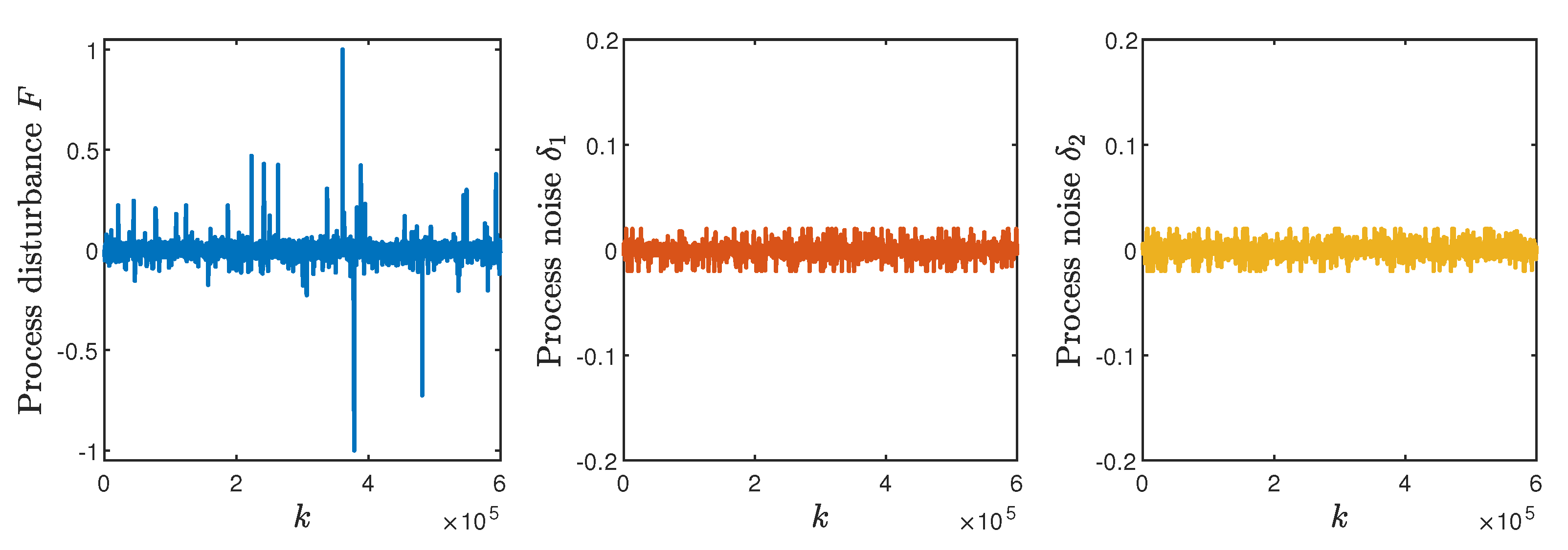
The horizons used in the DMC algorithm are: the prediction horizon , the control horizon and the horizon of process dynamics (the horizon of process dynamics is the number of step-response coefficients taken into account by the model used in the DMC algorithm) [39]. All values of the weights that penalise the excessive increments of the manipulated variables, i.e., , are equal to one. In this work, the objective of the controller is to effectively compensate the influence of three types of disturbances: changes of the flow rate of the input stream F, as well as the measurement noise of the first and the second process outputs, denoted as and , respectively. As many as 600,000 min (samples) are considered, i.e., approximately 417 days. It must be emphasised that in this work, the disturbances are not generated artificially, but real industrial disturbances recorded in a distillation process are used [39]. All 600,000 samples of the disturbances are shown in Figure 2.
All coefficients for , [39]. The problem to solve is to carefully select the tuning parameters for , . For this purpose, the tuning procedure presented in Section 3 is used.
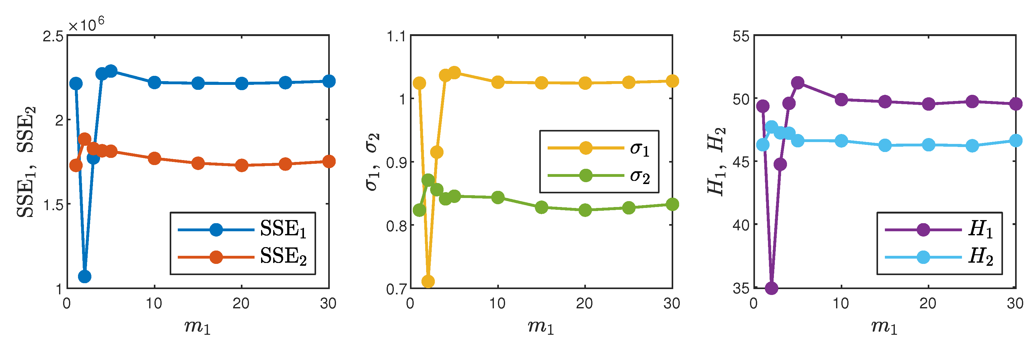
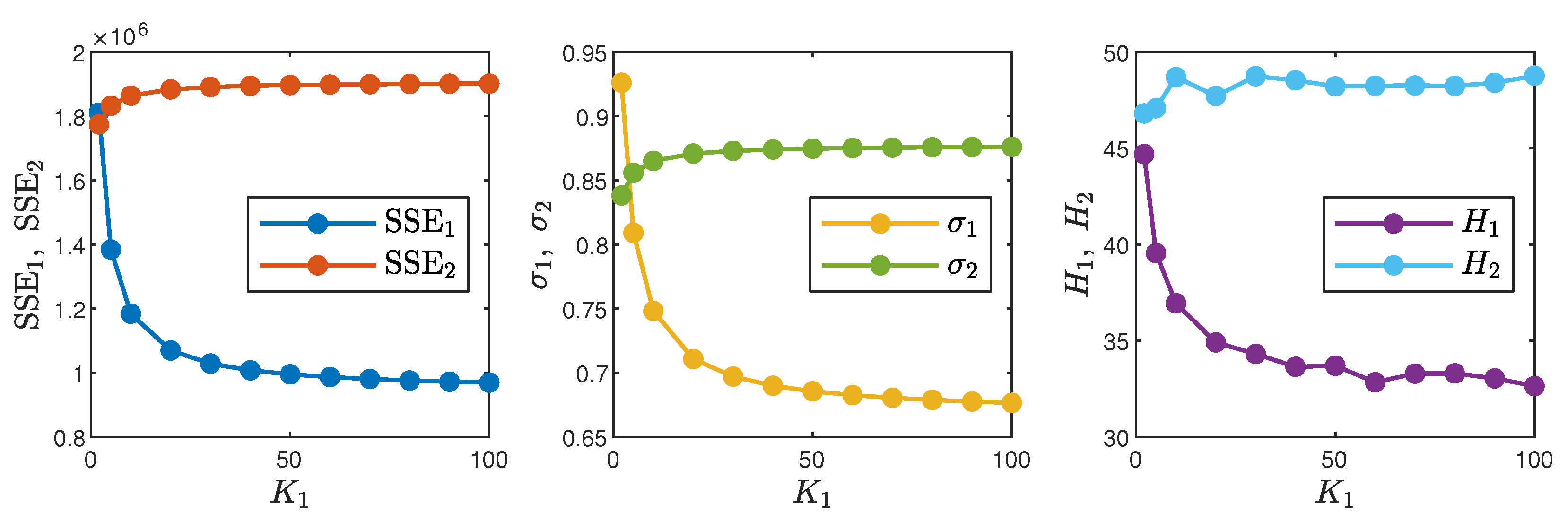
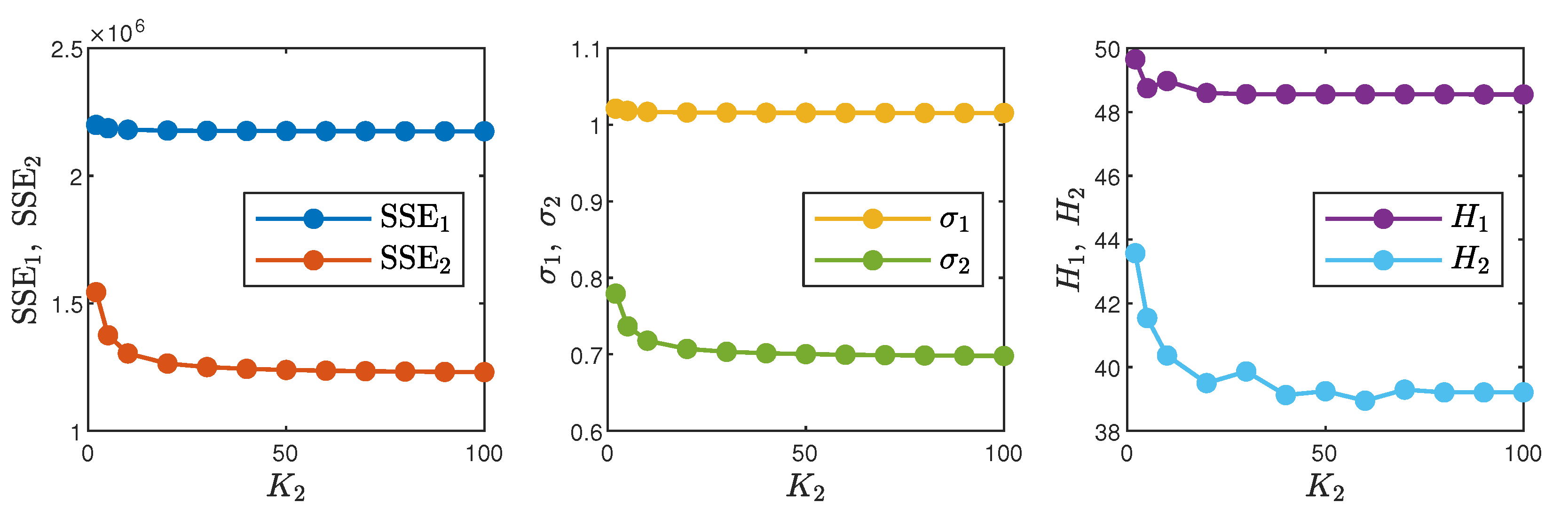
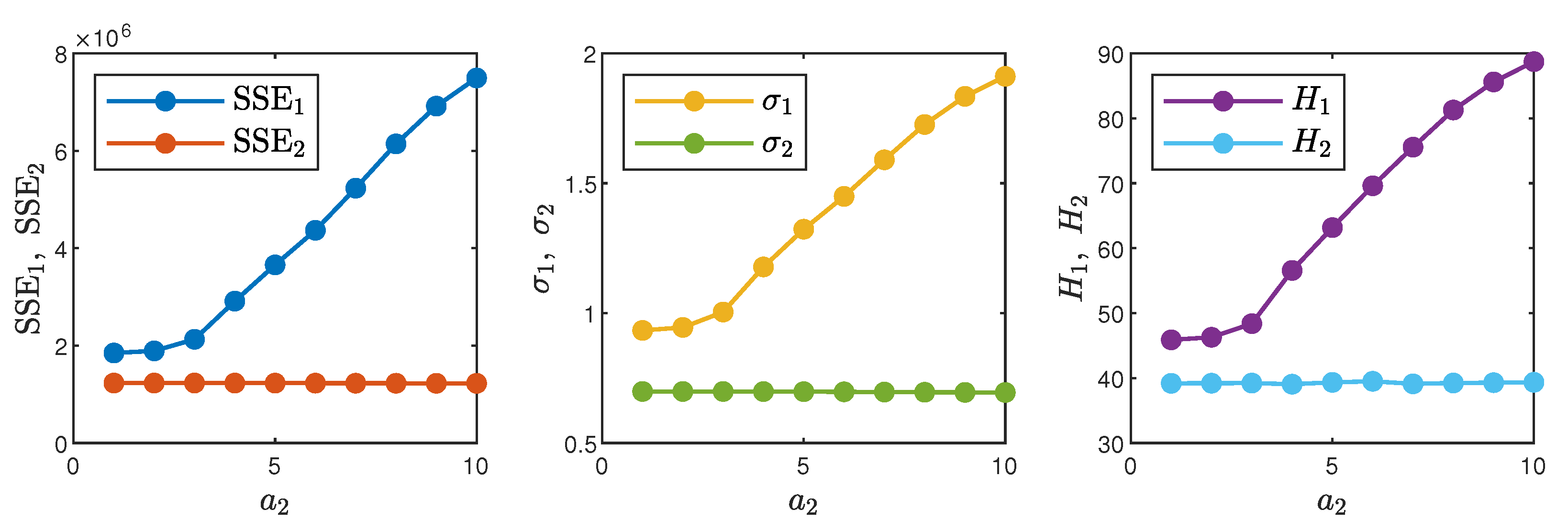
Let us first concentrate on tuning the coefficients , i.e., for the first process output, . Initially, the trajectory of the weights is parameterised by means of Equation (5), which is characterised by the parameters and . In the first step of the tuning procedure, the influence of the coefficient on the performance criteria , , , , and is analysed, and the results are shown in Figure 3. We take into account all three criteria for the first process output, i.e., the indices , and , and we choose the value because it gives the best control quality. Next, for the chosen parameter , in the second step, we assess the influence of the parameter , and it is shown in Figure 4. It is clear that the best results are obtained for . Finally, the trajectory of the weights is parameterised by means of Equation (6), which is characterised by the parameter as well as the fixed parameters and . Figure 5 depicts the influence of the parameter on the considered performance indices. The best set of control quality criteria is obtained for .
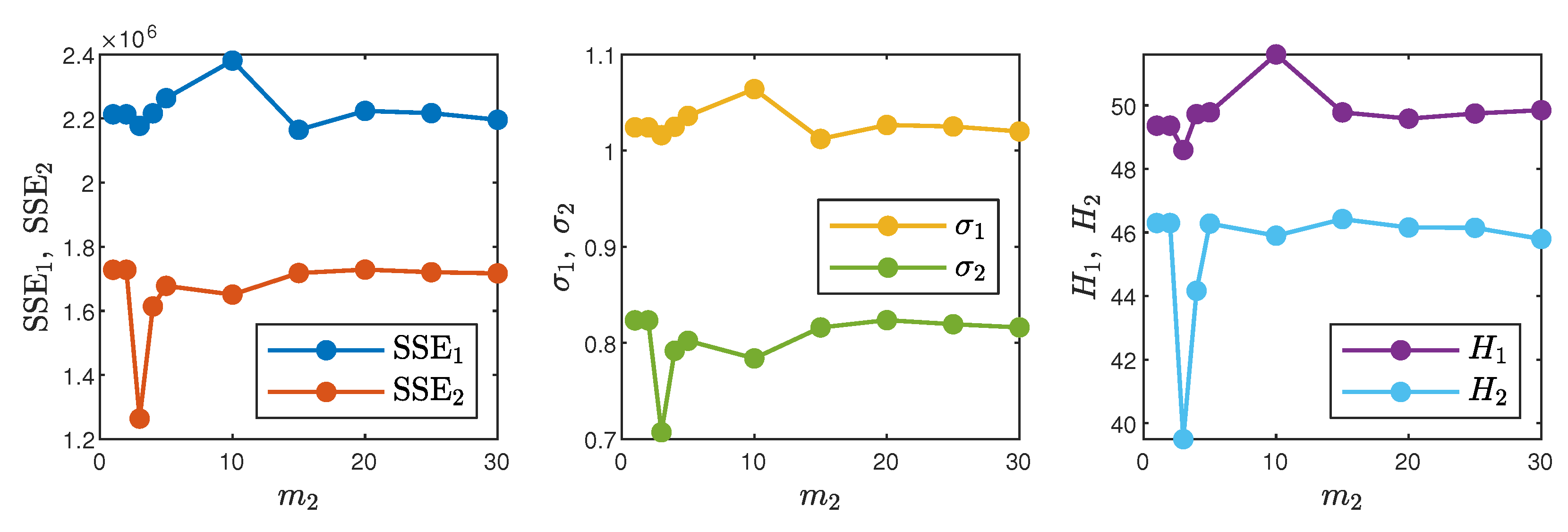
Next, having tuned the coefficients , let us concentrate on tuning the coefficients , i.e., for the second process output, . In the first step of the tuning procedure, the influence of the coefficient on the performance criteria is analysed, and the results are shown in Figure 6. We take into account all three criteria for the first process output, i.e., the indices , and . We easily find the best value . Next, for the chosen parameter , in the second step, we assess the influence of the parameter , and it is shown in Figure 7. It is clear that the best results are obtained for . Finally, Figure 8 depicts the influence of the parameter on the considered performance indices. The best results are obtained for .
All things considered, the coefficients are characterised by the set of parameters , and , while the coefficients by the parameters , and . The actual values of the coefficients used in MPC optimisation are computed from Equation (6).
To evaluate the efficiency of the chosen parameters and , let us consider the values of all six performance criteria. We not consider only the found coefficients, but additionally, we take into account the most practically cases in which all coefficients are constant, i.e., . In the latter case, we consider six values of the coefficients: 0.1, 1, 10, 100, 1000 and 10,000. The values of the obtained performance criteria are given in Table 1. For almost all considered indices (the only exception is , but the difference is not significant), the discussed tuning method gives the best results. For constant weights greater than 10,000, the results do not change.
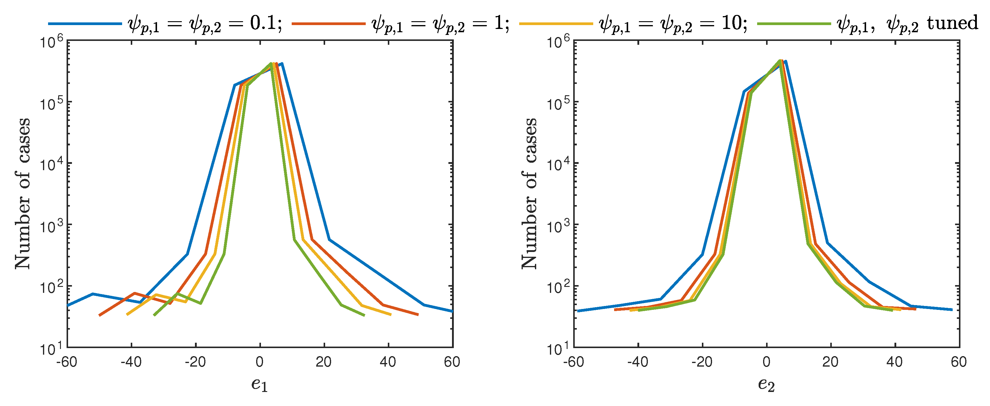
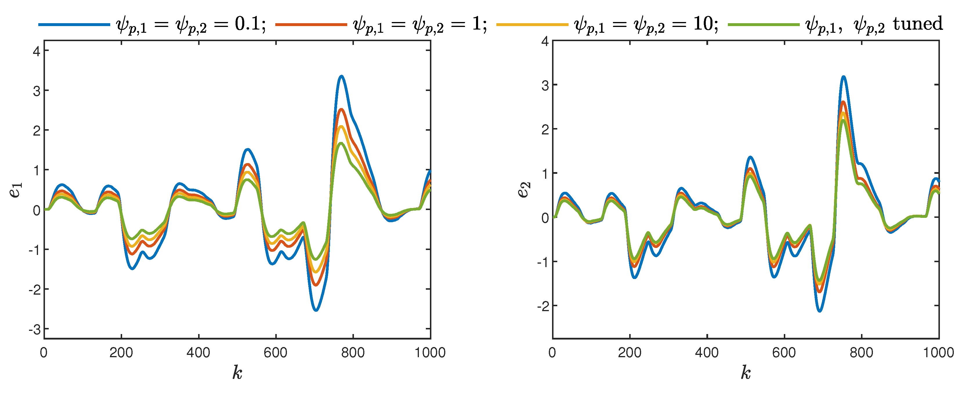
Let us now consider histograms of the control errors for constant values of the coefficients , and for the tuned ones. They are shown in Figure 9. Two observations are possible. Firstly, our tuning method gives the most narrow histograms. Secondly, they do not have long “tails”, which means that our method eliminates large negative and positive control errors. Figure 10 depicts the first 1000 samples of the control errors for constant values of the coefficients , and for the tuned ones. The obtained trends confirm the observations made on the basis of the histograms, i.e., our tuning method gives the best control quality.
In the second part of the simulations, we use the obtained set of tuning coefficients, but all gains of all input-output process channels are increased by 20%. Such a case is particularly interesting since the model used in MPC is (practically) never perfect. Table 2 shows the values of all six performance criteria. Additionally, we consider six cases in which all coefficients are constant and have the values 0.1, 1, 10, 100, 1000 and 10,000, respectively. For almost all considered indices (the only exception is , but the difference is not significant), the discussed method gives the best results. For constant weights greater than 10,000, the results do not change.
5. Conclusions
For MIMO processes, the classical optimisation approaches to finding the tuning parameters of MPC algorithms require very long vectors of decision variables. The resulting parameter optimisation task may be solved in simulations using some heuristic optimisation algorithms [12,32,33], but the huge computational complexity of such an approach in practice is an issue (the number of decision variables is large). This work presents a computationally simple approach to tuning of MPC parameters. The coefficients are not optimised directly, but they are parameterised. Moreover, the parameters are not calculated at the same time, but always, only one parameter is optimised. Multicriteria control quality assessment is possible. In this work, the following three indices are used: the sum of squared errors, the Huber standard deviation and the rational entropy. Unlike fully-fledged optimisation-based tuning methods, in our simulation-based approach, we simply assess how the consecutive parameters influence the value of the performance indices, and we choose the parameters for which the best results are possible. No numerical optimisation is used. The resulting tuning procedure is suboptimal, but our procedure is deliberately rather uncomplicated and is recommended to be used in industrial applications in which all tuning parameters are usually constant.
The efficiency of the discussed tuning method is demonstrated for a simulated MIMO distillation column. The classical process control task is considered, which is the compensation of the influence of the disturbances. It is shown that the discussed tuning method makes it possible to find the parameters that result in very good control quality, better than in the case of classical equal and large parameters. It is also shown that the determined set of parameters yields good control also in the imperfect model case.
Finally, let us stress the fact that our tuning method may be used to find parameters of numerous types of MPC algorithms. Classical MPC schemes based on linear models [6], as well as nonlinear ones [41] may be taken into account. Additionally, the constraints of different kinds may be included in the MPC optimisation problem.
Author Contributions
Conceptualization, R.N. and M.Ł.; methodology, R.N.; software, M.Ł.; validation, R.N. and M.Ł.; formal analysis, R.N.; investigation, R.N.; writing, original draft preparation, M.Ł.; writing, review and editing, R.N. and M.Ł.; visualization, M.Ł.; supervision, M.Ł. All authors read and agreed to the published version of the manuscript.
Funding
This research received no external funding.
Institutional Review Board Statement
Not applicable.
Informed Consent Statement
Not applicable.
Data Availability Statement
Data is contained within the article.
Conflicts of Interest
The authors declare no conflict of interest.
Nomenclature
| the spread of the Gauss function | |
| the control error of the nth process output | |
| the MPC cost function | |
| the parameter that defines the maximum value of the functions (5) and (6) | |
| MIMO | Multiple-Input Multiple-Output |
| the parameter that defines for which sampling instant p the Functions (5) and (6) have the value of | |
| N | the prediction horizon |
| the control horizon | |
| the number of process inputs | |
| the number of process outputs | |
| SISO | Single-Input Single-Output |
| , | the vectors that define the minimal and maximal values of the process inputs |
| , | the predicted value for the nth process output and the predicted vector for the sampling instant calculated at the current sampling instant k |
| , | the set point value for the nth process output and the set-point vector for the sampling instant known at the current sampling instant k |
| , | the vectors that define the minimal and maximal predicted values of the process outputs |
| , | the increment of the nth process input and the increment of the input vector for the sampling instant calculated at the current sampling instant k |
| decision variable vector of the MPC algorithm | |
| , | the vectors that define the minimal and maximal changes of the process inputs |
| the weighting matrix related to the change of the signal | |
| the weighting coefficient related to the change of the signal | |
| the weighting matrix related to the predicted control error | |
| the weighting coefficient related to the predicted control error |
References
- Balaska, H.; Ladaci, S.; Djouambi, A.; Schulte, H.; Bourouba, B. Fractional order tube model reference adaptive control for a class of fractional order linear systems. Int. J. Appl. Math. Comput. Sci. 2020, 30, 23–34. [Google Scholar]
- Salazar, J.C.; Sanjuan, A.; Nejjari, F.; Sarrate, R. Health-aware and fault-tolerant control of an octorotor UAV system based on actuator reliability. Int. J. Appl. Math. Comput. Sci. 2020, 30, 47–59. [Google Scholar]
- Bania, P. An information based approach to stochastic control problems. Int. J. Appl. Math. Comput. Sci. 2020, 30, 47–59. [Google Scholar]
- Salcedo, J.V.; Martínez, M.; García-Nieto, S.; Hilario, A. T-S fuzzy BIBO stabilisation of non-linear systems under persistent perturbations using fuzzy Lyapunov functions and non-PDC control laws. Int. J. Appl. Math. Comput. Sci. 2020, 30, 529–550. [Google Scholar]
- Maciejowski, J. Predictive Control with Constraints; Prentice Hall: Harlow, UK, 2002. [Google Scholar]
- Tatjewski, P. Advanced Control of Industrial Processes, Structures and Algorithms; Springer: London, UK, 2007. [Google Scholar]
- Plamowski, S.; Kephart, R.W. The model order reduction method as an effective way to implement GPC controller for multidimensional objects. Algorithms 2020, 13, 178. [Google Scholar] [CrossRef]
- Marusak, P.M. Numerically efficient fuzzy MPC algorithm with advanced generation of prediction—application to a chemical reactor. Algorithms 2020, 13, 143. [Google Scholar] [CrossRef]
- Assandri, A.D.; de Prada, C.; Rueda, A.; Martínez, J.S. Nonlinear parametric predictive temperature control of a distillation column. Control. Eng. Pract. 2013, 21, 1795–1806. [Google Scholar] [CrossRef]
- Morales-Rodelo, K.; Francisco, M.; Alvarez, H.; Vega, P.; Revollar, S. Collaborative control applied to BSM1 for wastewater treatment plants. Processes 2020, 8, 1465. [Google Scholar] [CrossRef]
- Gallego, A.J.; Merello, G.M.; Berenguel, M.; Camacho, E.F. Gain-scheduling model predictive control of a Fresnel collector field. Control Eng. Pract. 2019, 82, 1–13. [Google Scholar] [CrossRef]
- Ramasamy, V.; Sidharthan, R.; Kannan, R.; Muralidharan, G. Optimal tuning of model predictive controller weights using genetic algorithm with interactive decision tree for industrial cement kiln process. Processes 2019, 7, 938. [Google Scholar] [CrossRef] [Green Version]
- Pour, F.; Puig, V.; Ocampo-Martinez, C. Multi-layer health-aware economic predictive control of a pasteurization pilot plant. Int. J. Appl. Math. Comput. Sci. 2018, 28, 97–110. [Google Scholar] [CrossRef] [Green Version]
- Rahman, M.; Avelin, A.; Kyprianidis, K. An approach for feedforward model predictive control of continuous pulp digesters. Processes 2019, 7, 602. [Google Scholar] [CrossRef] [Green Version]
- Chatrattanawet, N.; Kheawhom, S.; Chen, Y.S.; Arpornwichanop, A. Design and implementation of the off-line robust model predictive control for solid oxide fuel cells. Processes 2019, 7, 918. [Google Scholar] [CrossRef] [Green Version]
- Takács, G.; Batista, G.; Gulan, M.; Rohal’-Ilkiv, B. Embedded explicit model predictive vibration control. Mechatronics 2016, 36, 54–62. [Google Scholar] [CrossRef]
- Kaleli, A. Development of the predictive based control of an autonomous engine cooling system for variable engine operating conditions in SI engines: Design, modeling and real-time application. Control Eng. Pract. 2020, 100, 104424. [Google Scholar] [CrossRef]
- Hou, X.; Guo, S.; Shi, L.; Xing, H.; Yin, H.; Li, Z.; Zhou, M. Improved model predictive-based underwater trajectory tracking control for the biomimetic spherical robot under constraints. Appl. Sci. 2020, 10, 8106. [Google Scholar] [CrossRef]
- Wang, Y.; Yu, H.; Che, Z.; Wang, Y.; Zeng, C. Extended State Observer-Based Predictive Speed Control for Permanent Magnet Linear Synchronous Motor. Processes 2019, 7, 618. [Google Scholar] [CrossRef] [Green Version]
- Sands, T. Comparison and interpretation methods for predictive control of mechanics. Algorithms 2019, 12, 232. [Google Scholar] [CrossRef] [Green Version]
- Chen, J.; Yu, Y.; Guo, Q. Freeway traffic congestion reduction and environment regulation via model predictive control. Algorithms 2019, 12, 220. [Google Scholar] [CrossRef] [Green Version]
- Lima, P.F.; Pereira, G.C.; Mårtensson, J.; Wahlberg, B. Experimental validation of model predictive control stability for autonomous driving. Control Eng. Pract. 2018, 81, 244–255. [Google Scholar] [CrossRef]
- Scattolini, R.; Bittanti, S. On the choice of the horizon in long-range predictive control–some simple criteria. Automatica 1990, 26, 915–917. [Google Scholar] [CrossRef]
- Seborg, D.E.; Edgar, T.F.; Mellichamp, D.A.; Doyle, F.J., III. Process Dynamics and Control; John Wiley & Sons: New York, NY, USA, 2011. [Google Scholar]
- Ionescu, C.; Copot, D. Hands-on MPC tuning for industrial applications. Bull. Pol. Acad. Sci. Tech. Sci. 2019, 67, 925–945. [Google Scholar]
- Garriga, J.L.; Soroush, M. Model predictive control tuning methods: A review. Ind. Eng. Chem. Res. 2010, 49, 3505–3515. [Google Scholar] [CrossRef]
- Shridhar, R.; Cooper, D.J. A tuning strategy for unconstrained multivariable model predictive control. Ind. Eng. Chem. Res. 1998, 37, 4003–4016. [Google Scholar] [CrossRef]
- Shridhar, R.; Cooper, D.J. A tuning strategy for unconstrained SISO model predictive control. Ind. Eng. Chem. Res. 1997, 36, 729–746. [Google Scholar] [CrossRef]
- Trierweiler, J.; Farina, L. RPN tuning strategy for model predictive control. J. Process Control 2003, 13, 591–598. [Google Scholar] [CrossRef]
- Yamashita, A.S.; Alexandre, P.M.; Zanin, A.C.; Odloak, D. Reference trajectory tuning of model predictive control. Control Eng. Pract. 2016, 50, 1–11. [Google Scholar] [CrossRef]
- Exadaktylos, V.; Taylor, C. Multi-objective performance optimisation for model predictive control by goal attainment. Int. J. Control. 2010, 83, 1374–1386. [Google Scholar] [CrossRef]
- Sawulski, J.; Ławryńczuk, M. Optimisation-based tuning of dynamic matrix control algorithm for multiple-input multiple-output processes. In Proceedings of the 2018 23rd International Conference on Methods & Models in Automation & Robotics (MMAR), Miedzyzdroje, Poland, 27–30 August 2018; pp. 160–165. [Google Scholar]
- Júnior, G.A.; Martins, M.A.F.; Kalid, R. A PSO-based optimal tuning strategy for constrained multivariable predictive controllers with model uncertainty. ISA Trans. 2014, 53, 560–567. [Google Scholar] [CrossRef]
- Nebeluk, R.; Marusak, P. Efficient MPC algorithms with variable trajectories of parameters weighting predicted control errors. Arch. Control. Sci. 2020, 30, 325–363. [Google Scholar]
- Nebeluk, R.; Ławryńczuk, M. Tuning of nonlinear MPC algorithm for vehicle obstacle avoidance. In Advanced, Contemporary Control; Bartoszewicz, A., Kabziński, J., Kacprzyk, J., Eds.; Springer: Cham, Switzerland, 2020; Volume 1196, pp. 993–1005. [Google Scholar]
- Domański, P. Control Performance Assessment: Theoretical Analyses and Industrial Practice. In Control Performance Assessment: Theoretical Analyses and Industrial Practice; Springer: Cham, Switzerland, 2020; Volume 245. [Google Scholar]
- Domański, P.D. Performance assessment of predictive control—A survey. Algorithms 2020, 13, 97. [Google Scholar] [CrossRef] [Green Version]
- Cutler, C.R.; Ramaker, B.L. Dynamic matrix control–A computer control algorithm. In Proceedings of the AIChE National Meeting, Denver, CO, USA, 17–21 June 1979. [Google Scholar]
- Domański, P.; Ławryńczuk, M. Multi-criteria control performance assessment method for a multivariate MPC. In Proceedings of the American Control Conference (ACC 2020), Denver, CO, USA, 1–3 July 2020; pp. 1968–1973. [Google Scholar]
- Wood, R.K.; Berry, M.W. Terminal composition control of binary distillation column. Chem. Eng. Sci. 2019, 28, 1707–1717. [Google Scholar] [CrossRef]
- Ławryńczuk, M. Computationally Efficient Model Predictive Control Algorithms: A Neural Network Approach. In Studies in Systems, Decision and Control; Springer: Cham, Switzerland, 2014; Volume 3. [Google Scholar]
Figure 1.
The flowchart of the tuning procedure.
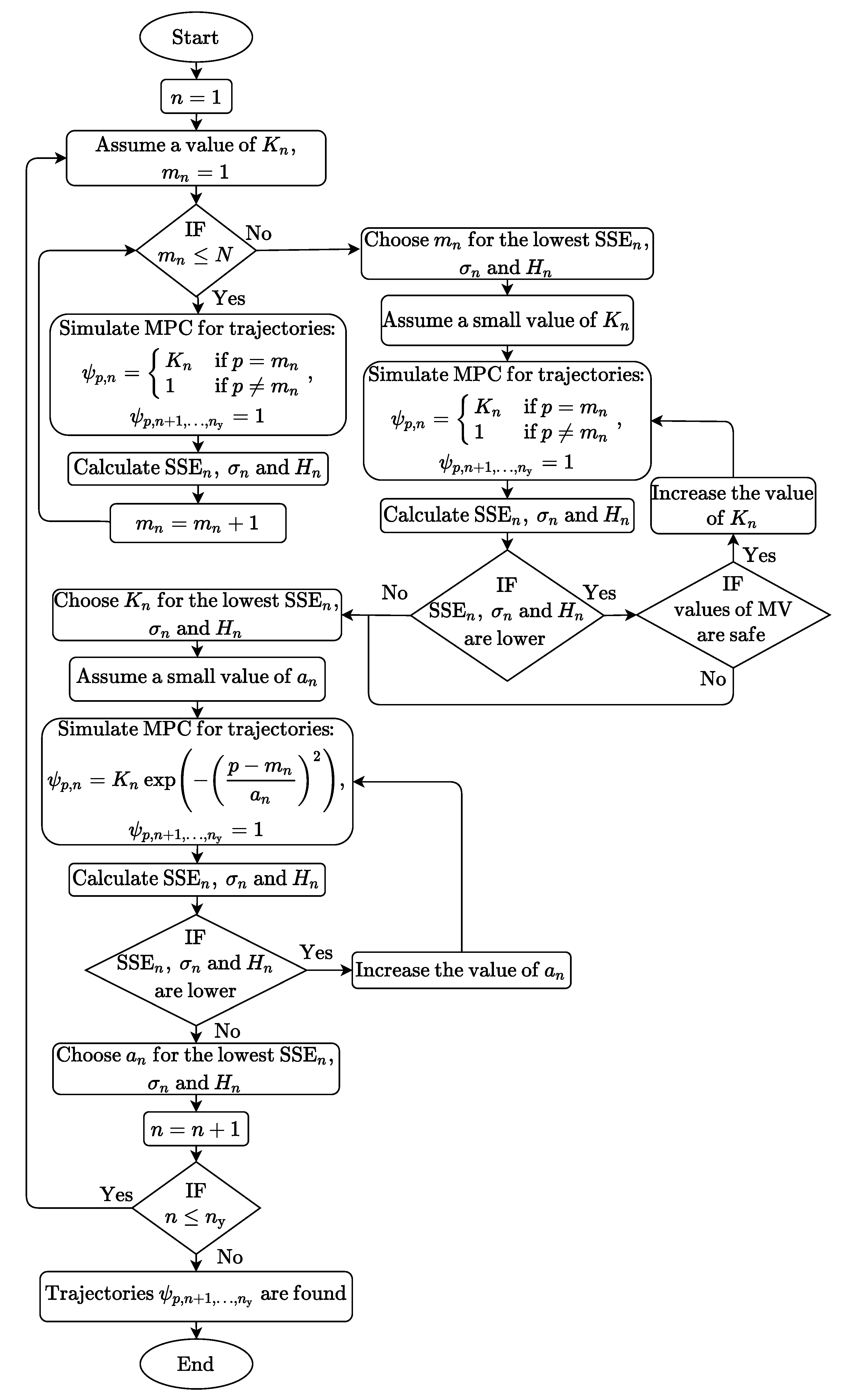
Figure 2.
All 600,000 samples of the disturbances.

Figure 3.
The first step of tuning the coefficients : the influence of the coefficient on the performance criteria , , , , and (for all 600,000 samples).
Figure 3.
The first step of tuning the coefficients : the influence of the coefficient on the performance criteria , , , , and (for all 600,000 samples).

Figure 4.
The second step of tuning the coefficients : the influence of the coefficient on the performance criteria , , , , and (for all 600,000 samples).
Figure 4.
The second step of tuning the coefficients : the influence of the coefficient on the performance criteria , , , , and (for all 600,000 samples).

Figure 5.
The third step of tuning the coefficients : the influence of the coefficient on the performance criteria , , , , and (for all 600,000 samples).
Figure 5.
The third step of tuning the coefficients : the influence of the coefficient on the performance criteria , , , , and (for all 600,000 samples).
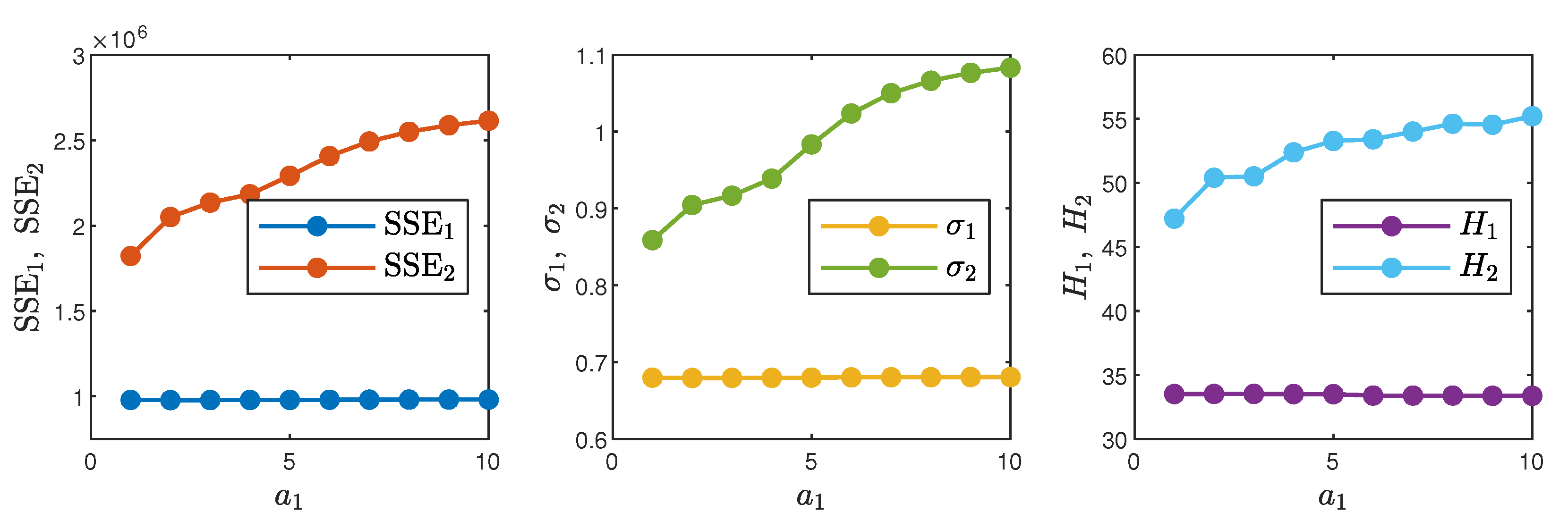
Figure 6.
The first step of tuning the coefficients : the influence of the coefficient on the performance criteria , , , , and (for all 600,000 samples).
Figure 6.
The first step of tuning the coefficients : the influence of the coefficient on the performance criteria , , , , and (for all 600,000 samples).

Figure 7.
The second step of tuning the coefficients : the influence of the coefficient on the performance criteria , , , , and (for all 600,000 samples).
Figure 7.
The second step of tuning the coefficients : the influence of the coefficient on the performance criteria , , , , and (for all 600,000 samples).

Figure 8.
The third step of tuning the coefficients : the influence of the coefficient on the performance criteria , , , , and (for all 600,000 samples).
Figure 8.
The third step of tuning the coefficients : the influence of the coefficient on the performance criteria , , , , and (for all 600,000 samples).

Figure 9.
The histograms of the control errors for constant values of the coefficients , and for the tuned ones (for all 600,000 samples).
Figure 9.
The histograms of the control errors for constant values of the coefficients , and for the tuned ones (for all 600,000 samples).
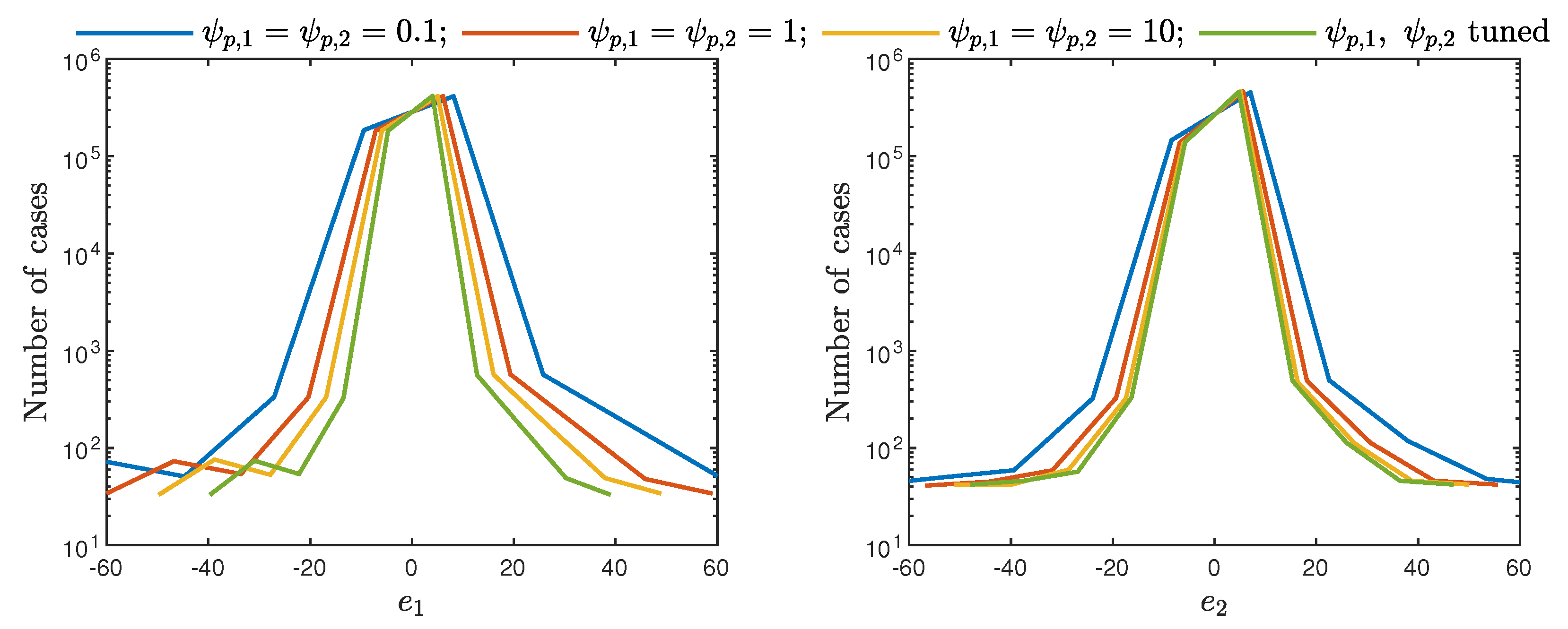
Figure 10.
The first 1000 samples of the control errors for constant values of the coefficients , and for the tuned ones.
Figure 10.
The first 1000 samples of the control errors for constant values of the coefficients , and for the tuned ones.
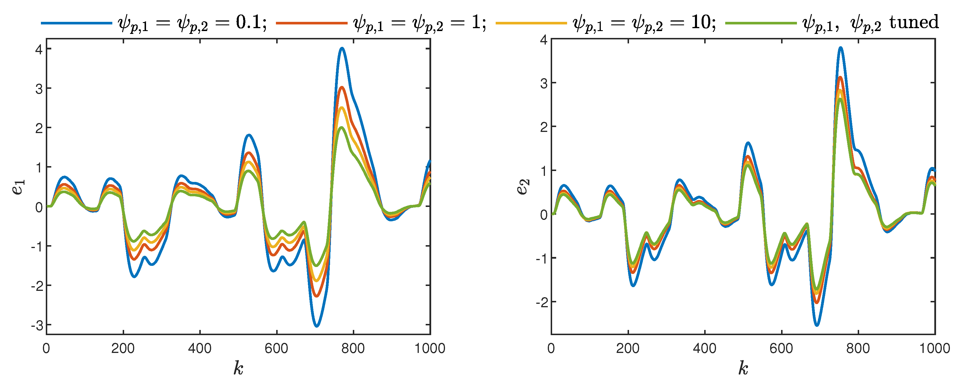
Figure 11.
The histograms of the control errors for constant values of the coefficients , and for the tuned ones (the imprecise model case, for all 600,000 samples).
Figure 11.
The histograms of the control errors for constant values of the coefficients , and for the tuned ones (the imprecise model case, for all 600,000 samples).

Figure 12.
The first 1000 samples of the control errors for constant values of the coefficients , and for the tuned ones (the imprecise model case).
Figure 12.
The first 1000 samples of the control errors for constant values of the coefficients , and for the tuned ones (the imprecise model case).


Table 1.
The values of the considered control quality indices for different constant parameters , , as well as for the tuned one (for all 600,000 samples).
Table 1.
The values of the considered control quality indices for different constant parameters , , as well as for the tuned one (for all 600,000 samples).
| Parameters | ||||||
|---|---|---|---|---|---|---|
| , tuned |
Table 2.
The values of the considered control quality indices for different constant parameters , , as well as for the tuned one (the imprecise model case, for all 600,000 samples).
Table 2.
The values of the considered control quality indices for different constant parameters , , as well as for the tuned one (the imprecise model case, for all 600,000 samples).
| Parameters | ||||||
|---|---|---|---|---|---|---|
| , tuned |
Publisher’s Note: MDPI stays neutral with regard to jurisdictional claims in published maps and institutional affiliations. |
© 2021 by the authors. Licensee MDPI, Basel, Switzerland. This article is an open access article distributed under the terms and conditions of the Creative Commons Attribution (CC BY) license (http://creativecommons.org/licenses/by/4.0/).
Share and Cite
MDPI and ACS Style
Nebeluk, R.; Ławryńczuk, M. Tuning of Multivariable Model Predictive Control for Industrial Tasks. Algorithms 2021, 14, 10. https://0-doi-org.brum.beds.ac.uk/10.3390/a14010010
AMA Style
Nebeluk R, Ławryńczuk M. Tuning of Multivariable Model Predictive Control for Industrial Tasks. Algorithms. 2021; 14(1):10. https://0-doi-org.brum.beds.ac.uk/10.3390/a14010010
Chicago/Turabian StyleNebeluk, Robert, and Maciej Ławryńczuk. 2021. "Tuning of Multivariable Model Predictive Control for Industrial Tasks" Algorithms 14, no. 1: 10. https://0-doi-org.brum.beds.ac.uk/10.3390/a14010010
Note that from the first issue of 2016, this journal uses article numbers instead of page numbers. See further details here.