A Bayesian Nonparametric Learning Approach to Ensemble Models Using the Proper Bayesian Bootstrap


1
Department of Mathematics, University of Pavia, 27100 Pavia, Italy
2
Department of Political and Social Sciences, University of Pavia, 27100 Pavia, Italy
3
Department of Decision Sciences, Bocconi University, 20100 Milano, Italy
*
Author to whom correspondence should be addressed.
†
These authors contributed equally to this work.
Algorithms 2021, 14(1), 11; https://0-doi-org.brum.beds.ac.uk/10.3390/a14010011
Submission received: 9 December 2020
/
Revised: 21 December 2020
/
Accepted: 29 December 2020
/
Published: 3 January 2021
(This article belongs to the Special Issue Bayesian Networks: Inference Algorithms, Applications, and Software Tools)
Abstract
:Bootstrap resampling techniques, introduced by Efron and Rubin, can be presented in a general Bayesian framework, approximating the statistical distribution of a statistical functional , where F is a random distribution function. Efron’s and Rubin’s bootstrap procedures can be extended, introducing an informative prior through the Proper Bayesian bootstrap. In this paper different bootstrap techniques are used and compared in predictive classification and regression models based on ensemble approaches, i.e., bagging models involving decision trees. Proper Bayesian bootstrap, proposed by Muliere and Secchi, is used to sample the posterior distribution over trees, introducing prior distributions on the covariates and the target variable. The results obtained are compared with respect to other competitive procedures employing different bootstrap techniques. The empirical analysis reports the results obtained on simulated and real data.
1. Introduction
Decision trees ([1]) are nonparametric predictive models used in regression and classification problems. Given a learning set where the represents the target variable, either categorical or numerical, and is a p dimensional vector of input variables, predictive models aim to make inference about an unknown function f that relates the target variable Y and the covariates vector . Decision trees work dividing the variables space into rectangles, making the final model easy interpretable. Despite their advantages in terms of results interpretability and predictive performance, decision trees are recognized to be an unstable procedure ([2,3]) and different ensemble techniques, based on Efron’s bootstrap procedure ([4]), have been proposed to improve stability.
Bagging classification and regression Trees ([2]) work generating a single predictor on different learning sets created by “bootstrapping” the original dataset and combining all of them to obtain the final prediction. Random Forests algorithm ([5,6]) employs bagging procedure coupled with a random selection of features, thus controlling the model variance and improving its stability. On the other hand, in Boosting techniques ([7,8]) the distribution of each training set, on which single models are trained, is based on the performance of previous predictors: the final prediction is obtained as a linear combination of single models, weighted using their performance errors.
In the Bayesian framework, Bayesian CART model ([9]) computes the final prediction using a linear combination of trees, in particular, the posterior distribution of a Bayesian single tree model is obtained averaging the resulting predictions weighted according to posterior probabilities. BART model ([10]) is the sum of M different tree models defined assigning a prior on the tree structure. BART model is extended in [11] to reduce the computational cost and provide a Bayesian competitive prediction result with respect to the Random Forests algorithm.
More recently, Bayesian nonparametric learning has been recognised as a good approach to solve predictive problems, overcoming the main weaknesses of parametric Bayesian models which assume fixed-dimensional probabilistic distributions ([12]). In [13], a Bayesian nonparametric procedure based on the Rubin’s bootstrap technique ([14]) is proposed to obtain a new class of algorithms called by the authors Bayesian Forests, under the idea that ensemble tree models can be represented as a sample from a posterior distribution over trees. Rubin’s bootstrap has been discussed as bagging procedure for different prediction models also in [15,16], proving that Bayesian bootstrap lead to more stable prediction results in particular with small sample sized datasets.
We remark that ensemble tree models based on Efron’s and Rubin’s bootstraps ([4,14]) are both non informative procedures since they do not take into account apriori knowledge (i.e., they build the prediction model just considering only observed values included in the data at hand and giving zero probability to values not available in the sample data). In addition these two procedures are proved to be asymptotically equivalent and first order equivalent from the predictive point of view ([17,18]).
The element of novelty of this paper is to introduce Proper Bayesian Bootstrap proposed by [19] in classification and regression ensemble trees models and compare the results obtained on simulated and real datasets with respect to classical bootstrap approaches available in the literature as Efron’s and Rubin’s bootstraps. More precisely, Proper Bayesian bootstrap is used to sample the posterior distribution over trees, introducing prior distributions on the covariates and the target variable.
The main aim of this paper is to employ Proper Bayesian bootstrap method in the data generative process introducing an ensemble approach based on decision tree models. In this work, bootstrap resampling techniques are applied to approximate the posterior distribution of a statistical functional , where F is a random distribution function as defined in the Proper Bayesian bootstrap ([19]) and is a decision tree. Note that our methodological proposal inherits the main advantages of Bayesian nonparametric learning such as the flexibility and the computational strength, considering also prior opinions and thus overcoming the main drawbacks of Efron’s and Rubin’s bootstrap procedures. On the basis of the results achieved in simulated and real datasets, our approach provides a reliable gain in predictive performance regarding the stability of the model, coupled with a competitiveness in terms of prediction accuracy.
The paper is structured as follows: Section 2 describes the Bayesian nonparametric learning framework, Section 3 shows the extension of bootstrap techniques in the Bayesian nonparametric framework, Section 4 introduces our methodological proposal involving Proper Bayesian bootstrap procedure, Section 5 presents empirical evaluations of our method with respect to other ensemble learning models. Finally, conclusions and further ideas of research are reported in Section 6.
2. Bayesian Nonparametric Learning Using the Dirichlet Process
The aim of the Bayesian nonparametric learning, introduced by [12,20], is to estimate the data generative process without limiting the family of involved probability density functions to the one with finite-dimensional parameters. Different prior distributions are available in literature both parametrics and nonparametrics; in our approach the Dirichlet process ([21]) is adopted.
A Dirichlet process prior with parameter is described by two quantities: a baseline distribution function , which defines the “center” of the prior distribution, and a non negative scaling precision parameter k, which determines how the prior is concentrated around . It is well known that the Dirichlet process is conjugate ([21]): given a random sample from , the posterior distribution is again a Dirichlet process:
with
The parameter of the Dirichlet process, given the data, is then a convex combination of the prior guess and the empirical distribution function . If then a non informative prior on is considered. If the parameter of the posterior Dirichlet Process is reduced to .
In this case it is easy to compute the posterior distribution, by simple updating the parameters of the prior distribution. This important property allows to derive easily Bayesian nonparametric estimation of different functional of F, such as the mean, median and other quantiles.
It has to be noticed that infinite computational time is required to sample from the posterior distribution. Since is continuous, in order to approximate the posterior distribution, bootstrap techniques can be applied as explained in the next Section.
3. Bootstrap Techniques in Nonparametric Learning
Let be i.i.d. realizations from a random variable X, and a functional depending on the distribution of X. In order to generate the distribution of the estimator , repeated bootstrap replications are drawn from the sample at hand.
From a Bayesian perspective, the aim is to estimate the posterior of the statistic under interest. Refs [22,23] discuss the connection between Bayesian procedures and bootstrapping. Given exchangeable sequence of real random variables, defined on a probability space , De Finetti’s Representation theorem ensures the existence of a random distribution F conditionally on which the variables are i.i.d with distribution F. The bootstrap procedure approximates the unknown probability distribution F with a . In particular, we are interested in calculating the distribution of a statistic conditionally on the sequence
where X refers to the sequence of random variables . Using bootstrap methods, (3) can be approximated by
where is obtained using different approaches of bootstraps as the Efron’s bootstrap ([4]), Rubin’s bootstrap ([14]) and Proper Bayesian bootstrap ([19]).
3.1. Efron’s Bootstrap
The Efron’s bootstrap ([4]) can be considered as a generalization of the jackknife ([24]) and it consists in generating independently each bootstrap resample from the empirical distribution of . This procedure is equivalent to draw, for each bootstrap replication, a weights vector w for the observations from a Multinomial distribution with parameters , where is the identity matrix of dimension . In this way we obtain:
where and is the indicator function.
Efron’s procedure assumes that the sample cumulative distribution function is the population cumulative distribution function and, under this assumption, it generates a bootstrap replication with replacement from the original sample.
3.2. Rubin’s Bootstrap
In [14] an alternative bootstrap procedure, called Bayesian bootstrap, is introduced. In particular with this procedure the distribution F is approximated by:
where and are two random independent vectors and and is the indicator function.
Following the nonparametric approach explained in Section 2 the prior is assumed to be a Dirichlet process, thus the obtained posterior is again a Dirichlet process. In this case k is set equal to 0, such that the empirical cumulative density function approximates the distribution F, as in Efron’s bootstrap resampling. The main difference between the two methods is that in Rubin procedure the vectors of the weights are drawn from a Dirichlet distribution with parameters . On the other hand, this approach, due to its assumptions regarding the data generating process, has the great advantage of characterizing the posterior distribution of given , as a Dirichlet process with parameters .
3.3. Proper Bayesian Bootstrap
A generalization of the Bayesian bootstrap introduced by Rubin is proposed in [19,25], with the main advantage of introducing prior knowledge represented by a distribution function . Following [21], the prior of F is defined as a Dirichlet process where is a proper distribution function and k represents the level of confidence in the initial choice . The resulting posterior distribution for F, given a sample from F, is still a Dirichlet process with parameter . As a special case when the procedure is equivalent to the Rubin’s one. This bootstrap method allows to introduce explicitly prior knowledge on the data through the choice of and k. It is important to remark that, since is a function of F, an informative prior on F is an informative prior on .
When it is often difficult to derive analytically the distribution of . When is discrete with finite support one may produce a reasonable approximation on the distribution of by a Monte Carlo procedure obtaining i.i.d. samples from . If is not discrete, in order to compute the posterior distribution , a possible way proposed by [19] is to first approximate the parameter through , where is the empirical distribution of an i.i.d. bootstrap resample of size m generated from:
The bootstrap resample is generated from a mixture of the empirical distribution function of and . Let now define as a random distribution which, conditionally on the empirical distribution of , is a Dirichlet process . Thus, since is given by a mixture of Dirichlet processes, using [26], when the law of weakly converges to the Dirichlet process .
Algorithm 1 shows how to estimate (4).
The conditional distribution expressed in (3) is approximated deriving the empirical distribution function generated by , where B is the number of bootstrap resamples.
The Bayesian nonparametric approach based on Proper Bayesian bootstrap can be introduced in ensemble models as explained in Section 4.
| Algorithm 1: |
 |
4. Our Proposal: Bayesian Nonparametric Learning Applied to Ensemble Tree Modeling
In the context of ensemble tree models, the statistic of interest is a decision tree model. As explained in Section 3, an estimation of the posterior distribution of can be derived through bootstrap procedures. In [13] Rubin’s bootstrap is applied to estimate the posterior distribution for . Each tree is obtained fitting the model on the weighted dataset (whose weights are drawn from a Dirichlet distribution) and the obtained predictions are an approximation of the posterior mean.
This paper extends the contribution of [13] introducing the Proper Bayesian bootstrap proposed in [19]. As described in Section 3, the Proper Bayesian bootstrap needs a definition of a prior distribution for F. In our case F represents the distribution of the data at hand and is a Dirichlet process with parameters k and . In order to explain a response variable y given a vector of P covariates , the parameter of the Dirichlet process is a joint distribution depending both on .
Following [19] we sample from the posterior of using Algorithm 2.
| Algorithm 2: |
 |
The bootstrap resample is generated by a mixture of distributions of the prior guess and the empirical distribution . When a new observation of bootstrap resample is generated, a new vector of covariates is generated from the prior distributions defined for the covariates, then the new value of the response variable is associated on the basis of the prior distribution chosen to model the relation between the target variable and the covariates. As in the other ensemble procedure based on tree models, the proposed method can be applied both for regression and classification problems, just considering different prior distribution based on the nature of the data at hand.
The main difference, with respect to classical ensemble procedure (i.e., Bagging trees and Bayesian Forest), is that the prior allows to generate new observations, not contained in the training set, which can enrich our prediction model. The obtained bootstrap samples are less dependent one to each other, thus obtaining a model which is less sensitive to changes in the learning dataset reducing overfitting. For this reason the obtained model is more stable and the error prediction benefits from a lower variance, as shown in Section 5.
5. Empirical Analysis
In this Section a sensitivity analysis on the parameters of the model introduced in Section 4 is performed choosing different prior distributions and setting different values of k (i.e., the level of confidence in our initial choice ). Our contribution, described in Section 4, is compared to Bagging algorithms based on Efron’s bootstrap and on Rubin’s bootstrap, respectively used in [2,13]. Empirical evidences and results about the prediction accuracy of the methods under comparison are provided, with the aim of investigating the properties of Proper Bayesian bootstrap in ensemble tree models. In details, each time a new dataset is analysed, the model is build on a different training set and a validation set (containing data not used in the model building phase) is used to evaluate their performance. The three different methods are evaluated observing the resulting mean squared error (MSE), the squared bias and the model variance. The squared bias evaluates the error in terms of erroneous assumptions in the learning algorithm while the model variance evaluates the stability of the model and is an estimation of the sensitivity of the model to small fluctuations in the training set. These two quantities are estimated, respectively, as:
where is the value of an observed y in the validation set estimated by the trained model. The sum of these two values gives the MSE, that is a general measure of quality of an estimator. The models are applied, first, on a simulated dataset to perform a bias-variance analysis of our prediction output, and finally results on a real dataset are reported.
For sake of comparison the number of bootstrap resamples B, and as a consequence the number of trees developed for each ensemble model under comparison, is fixed to 100.
5.1. Simulation Study
The Friedman function ([27]) allows to generate simulated datasets to perform performance comparisons between different regression models. The Friedman function is generated using the following equation
where and .
To evaluate the bias-variance trade-off 100 different datasets of size N, which represent our training sets, have been simulated. A regression model has been developed for each training set and each model has been evaluated on a common validation set generated from Friedman example made up of 100 observations.
A sensitivity analysis is performed on the simulated dataset from three different point of view: first, results are compared changing the prior distribution of the covariates, secondly, the prior on the relation between covariates and response variable to generate the pseudo-samples is changed, finally performances are shown based on different values of k and different values of training set sample size N.
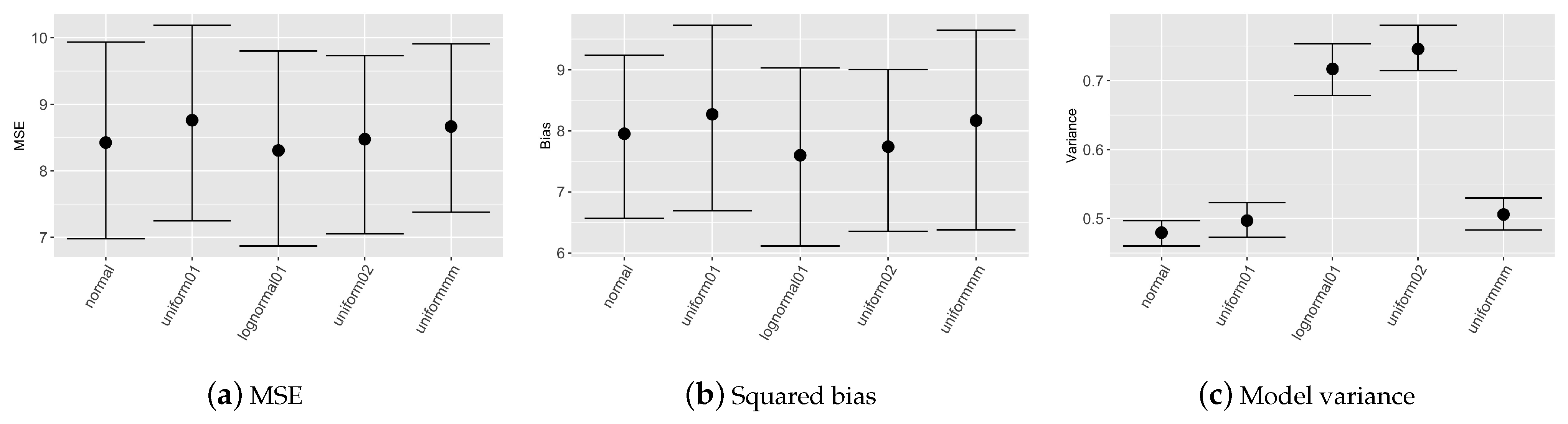
5.1.1. Empirical Evaluations Varying Prior on the Covariates
Figure 1 reports nonparametric confidence intervals evaluated on the 100 simulated datasets for mean squared error, squared bias and models variance considering different prior distributions for covariates. Table 1 describes the prior distributions chosen for the sensitivity analysis on the covariates prior choice. In this scenario the prior weight k is set to obtain considering that the sample size of the training set is composed of 100 observations. The prior relation between y and x is a nearest neighbour with . Figure 1 depicts, that MSE evaluated on the validation set is almost equal for all the prior choices; differences are evident in model variance, more precisely with prior set to or model results are less stable since variance shows higher values.
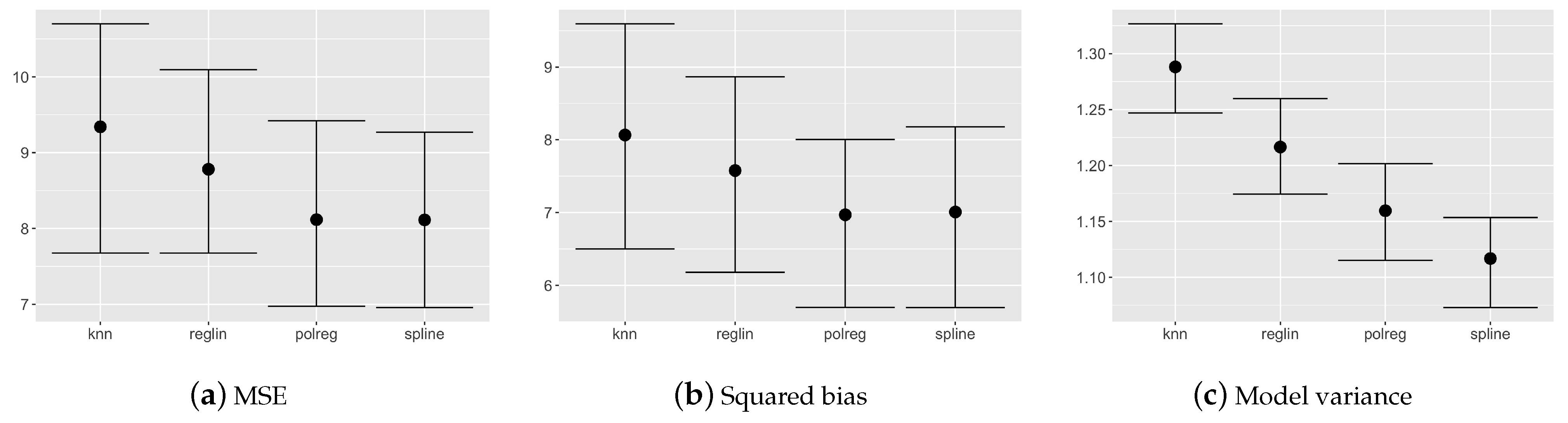
5.1.2. Empirical Evaluations Varying Prior on the Relation among x and y
The second approach on sensitivity analysis considers different prior models for the generation of the pseudo-dataset . In order to obtain the response variable , different prior regression models have been implemented as reported in Table 2. In this scenario we set the prior for each covariate as .
Figure 2 shows the results assuming the prior weight k as to obtain and a number of observations in the dataset equal to 100. The best results in terms of prediction accuracy come up using polinomial and spline regression. This is probably due to the nature of the simulated dataset. We remark that these differences are not statistically significant, thus we can say that the model is not sensitive to the prior choice.
5.1.3. Empirical Evaluations Varying k and Sample Size
The last exercise about sensitivity analysis considers different values of prior weights and different sample sizes of the training set. Figure 3, Figure 4 and Figure 5 show the results of the bootstrap confidence intervals for total mean squared error, squared bias and variance obtained on the validation set by the compared models: Efron’s bootstrap, Rubin’s bootstrap, Proper Bayesian bootstrap with different values of prior weight k (i.e., k such that the weight is equal to respectively: and ) and different sample sizes of the training set (i.e., , , ). In this simulation study, the prior for each covariate is set to and the prior relation among y and is a nearest neighbour with .
Figure 3 and Figure 4 show that the ensemble tree models outperform the single decision tree, as expected, even with different sample sizes of the training set. Values of the MSE and squared bias for the considered ensemble tree models are comparable, however, results obtained by the Proper Bayesian bootstrap present a slightly improvement especially for low values of the parameter k and low sample sized training set.
Figure 5 shows good results in terms of model stability. Ensemble tree models employing Proper Bayesian bootstrap seem to be the most stable models among the chosen ones, in particular when the value of w increases. If the weight given to the prior distribution is high, the bootstrap resamples include an higher number of new observations generated from the prior which enrich the original training set. As a consequence, the trees constructed for each bootstrap resample are more independent one from each other and the variance of the global ensemble model decreases. We can conclude that the proposed model is more stable, compared to other models introduced by [2,13] which employ different bootstrap techniques, while still remaining competitive in terms of prediction accuracy.
5.2. A Real Example: The Boston Housing Dataset
The Bayesian nonparametric algorithm introduced in this paper is also evaluated and compared to other models on a well known real dataset: the Boston housing dataset from the UCI repository [28]. The dataset is composed of 506 samples and 13 variables. The objective of this regression problem is to predict the value of prices of houses using variables at hand.
The training set is made up of the 70% of the observations (N) and the remaining part is taken as validation set on which mean squared error, bias and variance are evaluated. The model is built using a 10 fold cross validation.
The Uniform distribution is chosen as prior distribution for each covariate , and a k nearest neighbour with is used for the generation of the pseudo-samples in the Proper Bayesian bootstrap, as explained in previous sections.
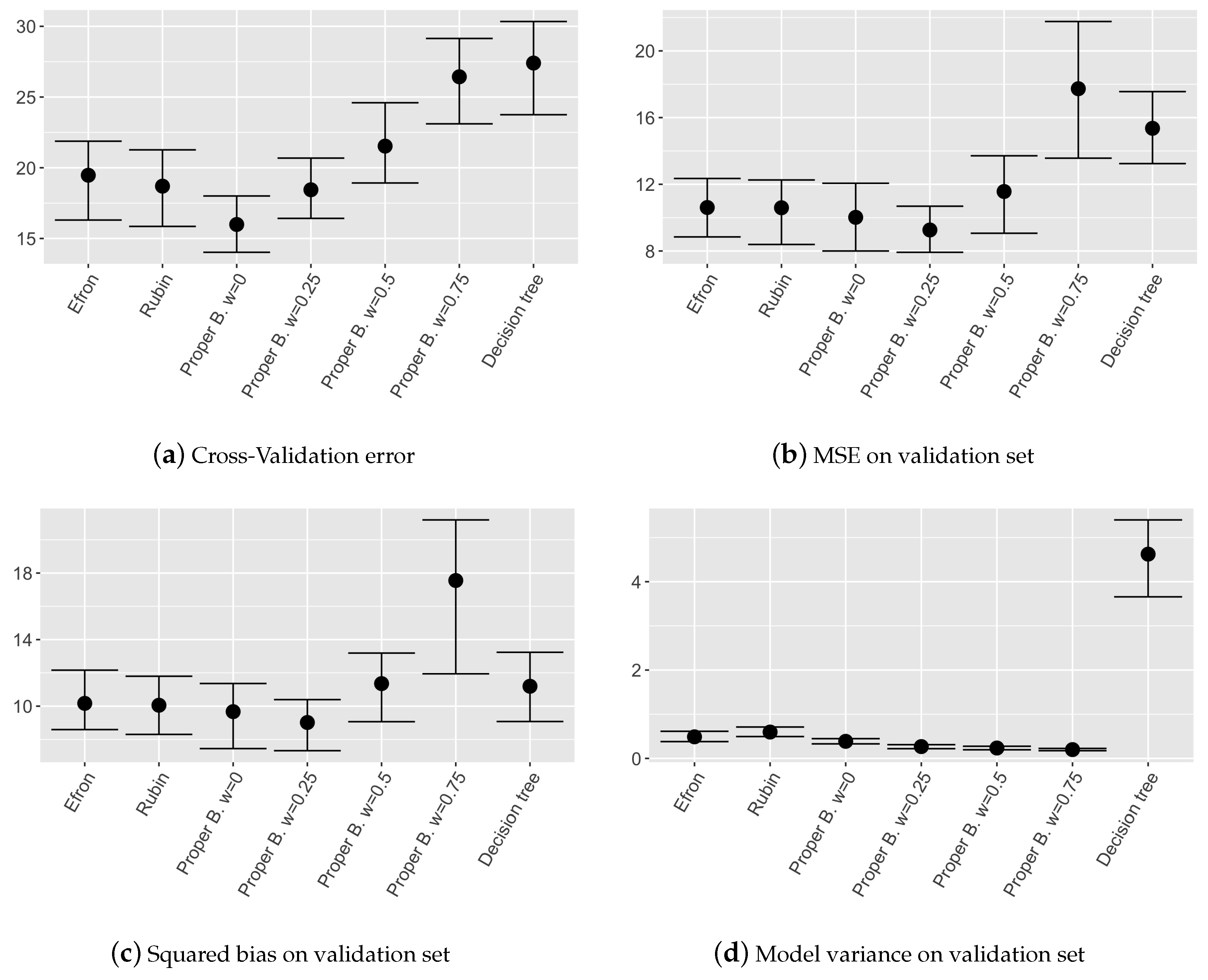
Results in terms of nonparametric confidence intervals evaluated on MSE, squared bias and variance of the different models are shown in Figure 6.
Observing the mean squared error on the validation set and the cross validation error, it can be noticed that the model involving Proper Bayesian bootstrap with low w performs as well as other ensemble models. While when w is high, i.e., prior is over weighted, the performances are influenced by the fact that in the dataset too many pseudo-samples are introduced.
As expected, observing the models variance in Figure 6d, it can be noticed that ensemble models are in general more stable than single decision tree and the models involving Proper Bayesian bootstrap are the most stable ones, as obtained in the simulated example. This is due to the higher independence among single trees given by the external pseudo-data introduced thanks to the prior distribution. We can conclude that also on real dataset the proposed model is more stable with respect to other ones employing different bootstrap techniques, maintaining a competitive level of accuracy.
6. Conclusions
In this paper a new approach in ensemble tree modelling using informative Bayesian bootstrap is proposed. In ensemble methods based on bagging, each data resample is generated through Efron’s bootstrap. This procedure is equivalent to consider the multinomial distribution as the prior distribution for the data generating process which assigns to each observation equal probability of being sampled. Under the Bayesian framework the natural extension is the bootstrap technique proposed by Rubin which considers the Dirichlet distribution as a prior distribution for the data generating process. It is well known that Efron’s and Rubin’s bootstraps are strongly dependent on the observed values and do not take into consideration any prior opinions.
In this paper the Proper Bayesian Bootstrap procedure is proposed in ensemble tree modelling. This procedure allows to introduce expert opinions through the definition of the prior parameter, thus overcoming the main drawbacks of the classical ensemble models which only consider the data without any prior opinion. However, if the prior distribution is not properly chosen, giving high weight to the prior could introduce noise in the data, thus loosing in model performance.
Obtained results suggest that, with the introduction of pseudo-samples in the data and a proper choice of prior weight, the final model can gain in terms of stability without loosing in model performance. These results are highlighted both in simulated and real datasets.
Author Contributions
Data curation, M.G.; Methodology, C.B.; Software, C.B.; Supervision, S.F. and P.M. All authors have read and agreed to the published version of the manuscript.
Funding
This research received no external funding.
Conflicts of Interest
The authors declare no conflict of interest.
References
- Breiman, L.; Friedman, J.; Olshen, R.A.; Stone, C.J. Classification and Regression Trees; Chapman & Hall: New York, NY, USA, 1984. [Google Scholar]
- Breiman, L. Bagging predictors. Mach. Learn. 1996, 24, 123–140. [Google Scholar] [CrossRef] [Green Version]
- Turney, P. Bias and the quantification of stability. Mach. Learn. 1995, 20, 23–33. [Google Scholar] [CrossRef] [Green Version]
- Efron, B. Bootstrap methods: another look at the jackknife. In Breakthroughs in Statistics; Springer: Berlin/Heidelberg, Germany, 1992; pp. 569–593. [Google Scholar]
- Ho, T.K. Random decision forests. In Proceedings of the 3rd International Conference on Document Analysis and Recognition, Montreal, QC, Canada, 14–16 August 1995; Volume 1, pp. 278–282. [Google Scholar]
- Breiman, L. Random forests. Mach. Learn. 2001, 45, 5–32. [Google Scholar] [CrossRef] [Green Version]
- Freund, Y.; Schapire, R.E. Experiments with a new boosting algorithm. In Proceedings of the 13th International Conference on Machine Learning, Bari, Italy, 3–6 July 1996; Volume 96, pp. 148–156. [Google Scholar]
- Friedman, J.H. Greedy function approximation: A gradient boosting machine. Ann. Stat. 2001, 29, 1189–1232. [Google Scholar] [CrossRef]
- Chipman, H.A.; George, E.I.; McCulloch, R.E. Bayesian CART model search. J. Am. Stat. Assoc. 1998, 93, 935–948. [Google Scholar] [CrossRef]
- Chipman, H.A.; George, E.I.; McCulloch, R.E. BART: Bayesian additive regression trees. Ann. Appl. Stat. 2010, 4, 266–298. [Google Scholar] [CrossRef]
- Hernández, B.; Raftery, A.E.; Pennington, S.R.; Parnell, A.C. Bayesian additive regression trees using Bayesian model averaging. Stat. Comput. 2018, 28, 869–890. [Google Scholar] [CrossRef] [PubMed]
- Lyddon, S.; Walker, S.; Holmes, C.C. Nonparametric learning from Bayesian models with randomized objective functions. In Proceedings of the Advances in Neural Information Processing Systems, Montréal, QC, Canada, 3–8 December 2018; pp. 2071–2081. [Google Scholar]
- Taddy, M.; Chen, C.S.; Yu, J.; Wyle, M. Bayesian and Empirical Bayesian Forests. In Proceedings of the International Conference on Machine Learning, Lille, France, 6–11 July 2015; pp. 967–976. [Google Scholar]
- Rubin, D.B. The Bayesian bootstrap. Ann. Stat. 1981, 9, 130–134. [Google Scholar] [CrossRef]
- Clyde, M.; Lee, H. Bagging and the Bayesian Bootstrap. In Proceedings of the AISTATS, Key West, FL, USA, 3–6 January 2001. [Google Scholar]
- Fushiki, T. Bayesian bootstrap prediction. J. Stat. Plan. Inference 2010, 140, 65–74. [Google Scholar] [CrossRef]
- Lo, A.Y. A large sample study of the Bayesian bootstrap. Ann. Stat. 1987, 15, 360–375. [Google Scholar] [CrossRef]
- Weng, C.S. On a second-order asymptotic property of the Bayesian bootstrap mean. Ann. Stat. 1989, 17, 705–710. [Google Scholar] [CrossRef]
- Muliere, P.; Secchi, P. Bayesian nonparametric predictive inference and bootstrap techniques. Ann. Inst. Stat. Math. 1996, 48, 663–673. [Google Scholar] [CrossRef]
- Fong, E.; Lyddon, S.; Holmes, C. Scalable Nonparametric Sampling from Multimodal Posteriors with the Posterior Bootstrap. In Proceedings of the International Conference on Machine Learning, Beach, CA, USA, 10–15 June 2019; pp. 1952–1962. [Google Scholar]
- Ferguson, T.S. A Bayesian analysis of some nonparametric problems. Ann. Stat. 1973, 1, 209–230. [Google Scholar] [CrossRef]
- Efron, B. Second thoughts on the bootstrap. Stat. Sci. 2003, 18, 135–140. [Google Scholar] [CrossRef]
- Efron, B. Bayesians, frequentists, and scientists. J. Am. Stat. Assoc. 2005, 100, 1–5. [Google Scholar] [CrossRef]
- Miller, R.G. The jackknife—A review. Biometrika 1974, 61, 1–15. [Google Scholar] [CrossRef]
- Muliere, P.; Secchi, P. Weak convergence of a Dirichlet-multinomial process. Georgian Math. J. 2003, 10, 319–324. [Google Scholar]
- Antoniak, C.E. Mixtures of Dirichlet processes with applications to Bayesian nonparametric problems. Ann. Stat. 1974, 2, 1152–1174. [Google Scholar] [CrossRef]
- Friedman, J.H. Multivariate adaptive regression splines. Ann. Stat. 1991, 19, 1–67. [Google Scholar] [CrossRef]
- Dua, D.; Graff, C. UCI Machine Learning Repository. 2017. Available online: https://archive.ics.uci.edu/ml/index.php (accessed on 2 January 2020).
Figure 1.
Comparison of nonparametric confidence intervals for MSE, squared bias and model variance related to the validation set for different prior choices on the covariates.
Figure 1.
Comparison of nonparametric confidence intervals for MSE, squared bias and model variance related to the validation set for different prior choices on the covariates.

Figure 2.
Comparison of nonparametric confidence intervals for mean squared error (MSE), squared bias and model variance related to the validation set for different prior choices on the relation among dependent and independent variables.
Figure 2.
Comparison of nonparametric confidence intervals for mean squared error (MSE), squared bias and model variance related to the validation set for different prior choices on the relation among dependent and independent variables.

Figure 3.
Nonparametric confidence intervals for MSE on the validation set varying N, number of observations in the training set.
Figure 3.
Nonparametric confidence intervals for MSE on the validation set varying N, number of observations in the training set.
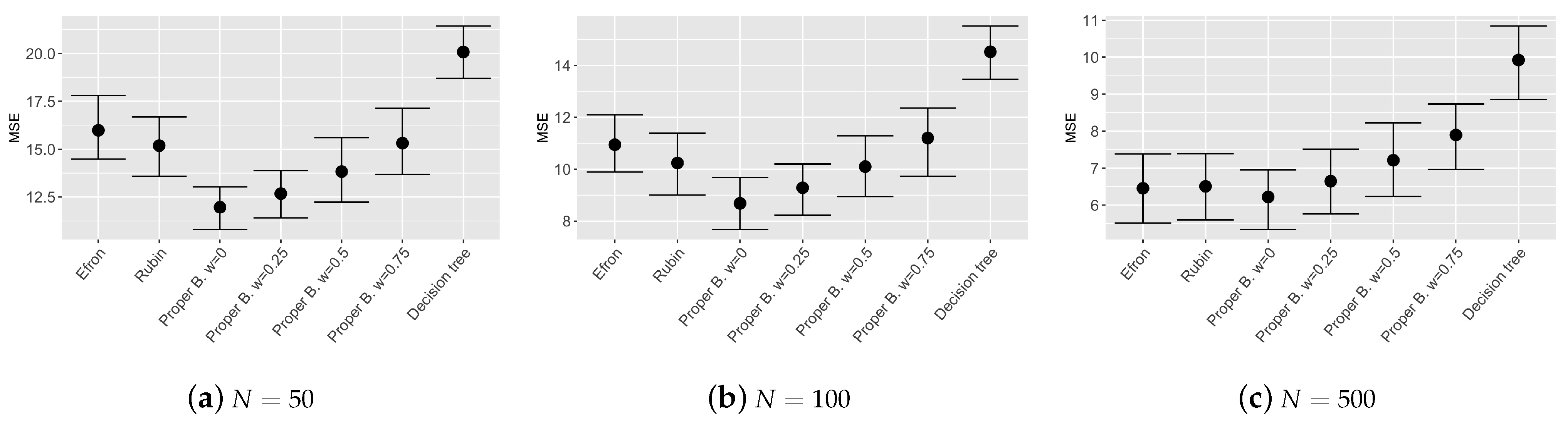
Figure 4.
Nonparametric confidence intervals for the squared bias on the validation set varying N, number of observations in the training set.
Figure 4.
Nonparametric confidence intervals for the squared bias on the validation set varying N, number of observations in the training set.
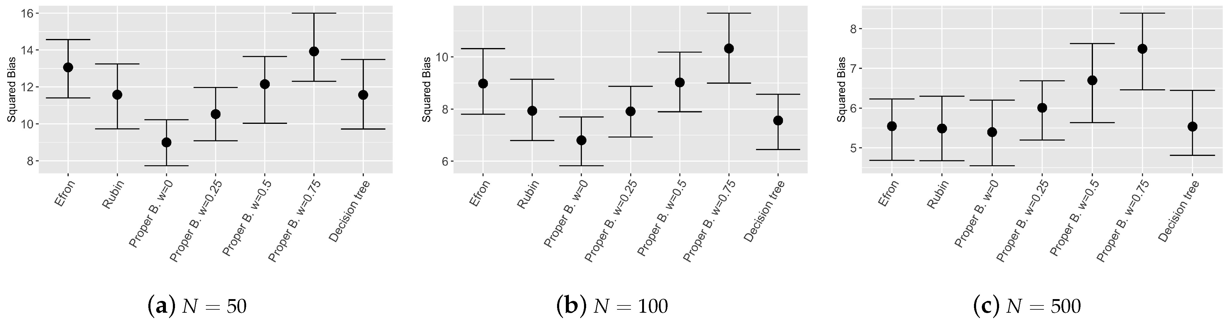
Figure 5.
Nonparametric confidence intervals for the variance on the validation set varying N, number of observations in the training set.
Figure 5.
Nonparametric confidence intervals for the variance on the validation set varying N, number of observations in the training set.
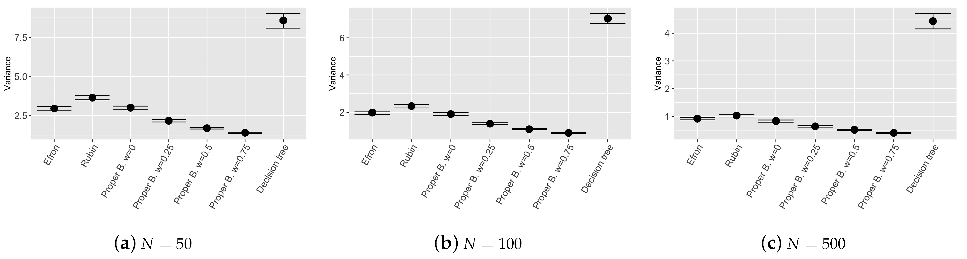
Figure 6.
Nonparametric confidence intervals on obtained results in real dataset.

Table 1.
Prior distribution for covariates.
| Plot Name | Prior Distribution |
|---|---|
| normal | |
| uniform01 | |
| lognorm01 | |
| uniform02 | |
| uniformmm |
Table 2.
Prior relation between response variable and covariates.
| Plot Name | Prior Distribution |
|---|---|
| knn | K-nearest neighbors with = 5 |
| reglin | Multiple linear regression |
| polreg | Polynomial regression with degree = 2 |
| spline | Spline regression |
Publisher’s Note: MDPI stays neutral with regard to jurisdictional claims in published maps and institutional affiliations. |
© 2021 by the authors. Licensee MDPI, Basel, Switzerland. This article is an open access article distributed under the terms and conditions of the Creative Commons Attribution (CC BY) license (http://creativecommons.org/licenses/by/4.0/).
Share and Cite
MDPI and ACS Style
Galvani, M.; Bardelli, C.; Figini, S.; Muliere, P. A Bayesian Nonparametric Learning Approach to Ensemble Models Using the Proper Bayesian Bootstrap. Algorithms 2021, 14, 11. https://0-doi-org.brum.beds.ac.uk/10.3390/a14010011
AMA Style
Galvani M, Bardelli C, Figini S, Muliere P. A Bayesian Nonparametric Learning Approach to Ensemble Models Using the Proper Bayesian Bootstrap. Algorithms. 2021; 14(1):11. https://0-doi-org.brum.beds.ac.uk/10.3390/a14010011
Chicago/Turabian StyleGalvani, Marta, Chiara Bardelli, Silvia Figini, and Pietro Muliere. 2021. "A Bayesian Nonparametric Learning Approach to Ensemble Models Using the Proper Bayesian Bootstrap" Algorithms 14, no. 1: 11. https://0-doi-org.brum.beds.ac.uk/10.3390/a14010011
Note that from the first issue of 2016, this journal uses article numbers instead of page numbers. See further details here.