Quantitative Spectral Data Analysis Using Extreme Learning Machines Algorithm Incorporated with PCA


Centre for Intelligent Systems and School of Engineering and Technology, Central Queensland University, Rockhampton, QLD 4701, Australia
*
Author to whom correspondence should be addressed.
Algorithms 2021, 14(1), 18; https://0-doi-org.brum.beds.ac.uk/10.3390/a14010018
Submission received: 3 December 2020
/
Revised: 5 January 2021
/
Accepted: 7 January 2021
/
Published: 11 January 2021
(This article belongs to the Special Issue Algorithms in Hyperspectral Data Analysis)
Abstract
:Extreme learning machine (ELM) is a popular randomization-based learning algorithm that provides a fast solution for many regression and classification problems. In this article, we present a method based on ELM for solving the spectral data analysis problem, which essentially is a class of inverse problems. It requires determining the structural parameters of a physical sample from the given spectroscopic curves. We proposed that the unknown target inverse function is approximated by an ELM through adding a linear neuron to correct the localized effect aroused by Gaussian basis functions. Unlike the conventional methods involving intensive numerical computations, under the new conceptual framework, the task of performing spectral data analysis becomes a learning task from data. As spectral data are typical high-dimensional data, the dimensionality reduction technique of principal component analysis (PCA) is applied to reduce the dimension of the dataset to ensure convergence. The proposed conceptual framework is illustrated using a set of simulated Rutherford backscattering spectra. The results have shown the proposed method can achieve prediction inaccuracies of less than 1%, which outperform the predictions from the multi-layer perceptron and numerical-based techniques. The presented method could be implemented as application software for real-time spectral data analysis by integrating it into a spectroscopic data collection system.
1. Introduction
Spectroscopy is one of the primary exploratory tools that have been used to study the micro-world, investigating the physical structure of substances at the atomic and molecular scale, and characterizing the properties of novel materials, as the physical structure and properties of substances at the micro-world scale cannot be directly measured or observed by any instruments. Through spectroscopic technology, it is possible to determine the key properties of matter such as compositions and electronic structures at the nano-level. There are some different spectroscopic techniques that can be used to reveal different properties and characteristics of materials. So far, several spectroscopic methods, like emission, absorption, Raman, and backscattering, etc., have been well developed. In this article, we mainly discuss the data analysis problem of the Rutherford backscattering spectroscopy (RBS). RBS is a physical process in which a beam of high energy incident ions is projected to a thin solid sample to be analyzed. The backscattering spectrum of the incident particles is recorded, which essentially is a noisy curve of the backscattering particle yield against the energy of scattered ions or the device channels. By a quantitative analysis of the RBS spectra, the elementary compositions and their depth profiles of substances are extracted. Conventionally, the problem of RBS spectral data analysis has been viewed as a numerical fitting problem, assisting with complementary knowledge in advanced physics. The solution by a numerical fitting procedure, generally starts with an initial guess on the sample structural information, and then calculates the theoretical spectral curve from the backscattering physics. The sum of mean-squared error between the theoretical spectra and measured spectroscopic data is minimized in an iteration process by a least-square algorithm. In the iteration process, the measured spectra and theoretical spectra are recursively compared, and the structural parameters are adjusted in the running computational program till a convincing match or a pre-set error value is achieved. The conventional numerical method has two major issues—(i) The convergence of minimizing error process is not guaranteed; and (ii) It highly relies on the analyst’s empirical skills and advanced physics knowledge.
The emergence of new algorithms in machine learning in decades, has inspired researchers’ passions and interests to attempt novel solutions based on optimization algorithms or intelligent techniques, such as simulated annealing, support vector machines, and artificial neural networks. Barradas and co-authors [1] proposed to apply the combinatorial optimization simulated annealing (SA) algorithm [2,3,4] to the analysis of RBS spectra. Their analysis method could be designed in a fully automatic manner, without human intervention on the parameter adjustments in the analysis process. The proposed method was tested on a few complicated physical samples, such as iron-cobalt silicide and SiOF spectra, and the sample structural parameters were correctly determined in terms of a quantitative way. In addition to the SA algorithm, the neural computing-based method was also considered to solve specific problems in RBS spectral data analysis. Barradas et al. [5,6,7] developed a multilayer perceptron (MLP) model with the spectrum as input and the sample structural parameters as output for the quantitative analysis of RBS data. The developed MLP model was strictly trained with thousands of theoretically generated spectra of the samples that have the known nominal structures. Then the well-trained MLP acquired a learning capability to interpret the spectrum of a given sample, for which the physical structure was unknown. Their numerical results showed the developed MLP model could quantitatively predict the sample structure with reasonable accuracies, provided a sufficient amount of training data. These investigations appear to be a great advancement toward developing a relatively easy data-driven analysis approach, without much expert knowledge involved.
However, it should mention that in Barradas’ method of using the neural network model, each RBS spectrum with up to several hundred data points was used as a single input, without a necessary dimensionality reduction. Such a method inevitably requires a huge amount of training data and a very long training time, which influences the convergence. This is a gap to be filled in our study by using a data dimensionality reduction technique.
We should emphasize that neural network models are not limited to solving data analysis problems in the domain of natural science. More commonly, neural networks and other methods of machine learning have been extensively applied to a wide range of disciplines, such as system identification and control [8], pattern recognition and classification [9], medical diagnosis [10,11,12], finance, and many others. The successes of using machine learning methods have been proven in these works, with significant improvement of classification and prediction accuracies. As a variation of single-hidden layer feed-forward neural network (SLFN), extreme learning machine (ELM) is a special SLFN network where input weights and biases of the hidden layer are randomly generated, and the output weights are analytically determined from input data [13]. Due to its fast learning capability and excellent generation performance, a large number of applications of ELM have been carried out in the past fifteen years [14,15,16,17,18]. There are several works [19,20,21] that apply ELMs to make classifications on food or wine associated with spectroscopic data or relevant feature selections. Zheng et al. [19,20] presented a study based on the combination of spectroscopy and ELM algorithm for food classification. Four benchmark spectroscopic datasets [22] involving food samples including coffee, olive oil, meat, and fruit, with corresponding measured near-mid infrared spectroscopy were used in their investigations. They also compared the experimental results from the ELM algorithm with those from other methods like back-propagation artificial neural networks (BP-ANN), k-nearest neighbor (KNN), and support vector machines (SVM). Their study shows the classification accuracies of ELM can be achievable up to 100%, 97.78%, 97.35%, and 95.05% for coffee, meat, olive oil, and fruit, respectively, which improved about 6% compared to other methods in addition to faster classification speed.
More recently, ELMs have appeared in a deep structure for investigating specific pattern recognition or object classification problems [23,24,25]. Different from the three-layer architecture of a single ELM, the multi-layered deep ELM can be constructed by stacking a series of standard ELM models with or without constraints. Khan et al. [23] designed and implemented a neural classifier based on deep ELMs for fabric weave pattern and yarn colour recognition and classification. They have reported that the deep ELM classifier significantly improved the classification error rates and achieved better recognition accuracy up to 97.5% [23] for complex weave patterns, whereas the recognition accuracies from other methods are between 80% and 84% for the same problem.
In this study, a universal method that incorporates neural networks and the dimensionality reduction technique has been proposed to explore a new approach for spectral data analysis. Our objectives include firstly transforming the complicated numerical computation problem into a multivariate regression problem associated with a learning process through datasets, secondly reducing data dimensionality in the input space for easier training and ensuring convergency, and thirdly utilizing extreme learning machines to establish a mapping mechanism using the reduced data components as input to produce an accurate prediction of the structural parameter information. This work contributes to a newly proposed method transforming conventional numerical analysis based problem into a statistical learning problem through data. The proposed method is a general-use approach for any spectra-oriented applications. It has been demonstrated by a set of RBS data with producing accurate predictions of the physical sample structures. This method significantly reduces the reliance on an initial guess and user intervention in the process of analyzing spectral data, which greatly alleviates the burden of analysts. It may be applicable for spectral analysis applications involving high volumes of data, even for automating the analyzing process in collecting real-time experimental spectra if a suitable interface between the spectrometer and application software is implemented properly.
2. Materials and Methods
2.1. Spectral Data Analysis and Multivariate Regression Problems
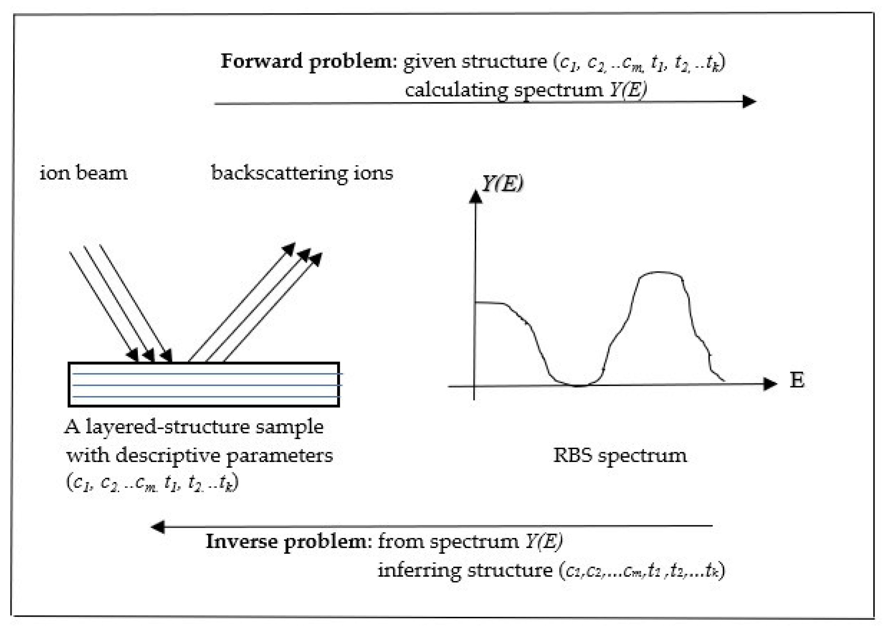
As discussed in the last section, RBS is a backscattering physical process. The relationship between cause and effect of a physical process can be described in terms of mathematical problems—the forward problem and the inverse problem. The forward problem starts with causes and gets the outcome by calculating the effects. On the contrary, the inverse problem is to give information on the outcome of a physical phenomenon or process, but it requires inferring the causes quantitatively. Parameters of a physical process are required to be defined in order to describe the “causes” in a quantitative manner. Forward problems in practice often can be solved satisfactorily by physics principles and computationally mathematical models if the relevant process and mechanism are well understood. However inverse problems usually are extremely difficult, since they generally are ill-posed and the solutions are non-unique [26,27]. There may exist a large solution space with many possible solutions that match the observed outcome. In certain circumstances, even a unique solution could be found to be accurate for a set of data, but it could be unstable to the perturbation of noise in the other observed dataset.
The problem of spectral data analysis can be defined as an inverse problem, because it gives a set of spectral data or measured spectroscopic curves and requires acquiring the cause—the values of the physical parameters governing the corresponding physical process by a computational method. Solving the inverse problems that are arisen in spectroscopy has significant importance because it is an effective means to secure the accurate values of the physical parameters related to the process. The diagram in Figure 1 illustrates the backscattering physical process and the formal definition of the inverse problem in the RBS data analysis.
It is obvious that the problem of calculating an RBS spectrum itself is a forward problem that computes the backscattering yield curve against energies or channels based on Rutherford’s theory for a given sample structure. The backscattering yield can be written as a multiple integral form as below [28],
where E is incident ion energy, Q, θ, and others are the related physical quantities; and ξ is the system noise.
In a compact form, the backscattering spectrum can be abstracted as a parametric function h(E,p)
where p represents the structural information parameter that describes the property of a physical sample to be analyzed. More specifically, for most RBS analysis problems, the structural parameter p can be flattened and written as a vector
where ci and tj (i = 1, 2, …, m; j = 1, 2, …, k) are atomic concentrations and thickness parameters of the sample, with total m compositions and k layers, and T refers to the transpose operation.
The actual task of RBS data analysis is that given a backscattering spectrum y(E), it requires securing the sample structural parameter p (i.e., compositional depth profile). This can be formulated as an inversion of Equation (3), which can be expressed into
where h−1(y) is an inversion function and the noise is combined in the spectrum y(E). On the contrary to the forward problem, there does not exist the analytical expression on the inversion function h−1(y). Despite the ill-posed property of the inverse problems, in terms of statistical learning perspective, we can transform the inverse problem as a multivariate regression problem as it has a lot of observation data from spectroscopy measurements for a statistical learning process. This can be re-depicted as the following form,
where fmodel(.) represents a multivariate nonlinear regression model with n explanatory variables which are the discretized spectral intensity values at energy positions El (l = 1, 2, …, n) with N observations. Thus a tough inverse problem is converted as a regression problem. As the neural network technique has been successfully applied to resolve many regression and classification problems, we proposed using a special class neural network named extreme learning machine (ELM) to approximate the nonlinear regression function where the spectrum is treated as input via n nodes and the structural parameter p vector is the output, and the built network constitutes a mathematical realization of the multivariate nonlinear regression model fimodel(y(E1), y(E2), …, y(En)), i = 1, 2, …, n. Through an efficient training and validation from the existing spectroscopic data with known structures, the unknown structural parameter for a new sample can be determined by a generalization process.
i = 1, 2, …, N
2.2. Solution by an Enhanced ELM
In statistical learning theory, an unknown nonlinear regression function can be approximated by a set of basis function expansions. This can be analytically expressed into [29,30]
where βi(x) is known as basis functions, and λi are expansion coefficients. Broomhead and Lowe [31] extended this concept by restricting the basis functions to the radial basis functions and applied it to resolve the multi-dimensional interpolation problems, in which each basis function was treated as an activation function in the node of the single hidden layer network, and therefore the Equation (7) is equivalent to a radial basis function (RBF) network with M neurons in the hidden layer. Due to its excellent analytical properties, the RBF network can approximate any continuous function to an arbitrary accuracy if a sufficiently large number of hidden nodes is provided [32]. The idea was further extended by allowing input weights and parameters of hidden layer nodes can be randomly assigned, which is called extreme learning machine (ELM), proposed by Huang et al. [13]. By denoting the output weight vector as w and the activation function as φ(x), the output function of the ELM can be expressed as
where a and b are the input weight vector and hidden layer node activation function parameters, with L hidden layer nodes. In practical applications, the Gaussian function is often chosen as the activation function. The Gaussian function is a typical localized function that decays quickly from the locations nearby its centers. As our previous studies indicated [33,34], by adding a linear neuron, it would efficiently reduce the localized effect and therefore improve the modeling accuracy. With the additional linear term, the enhanced version ELM output function can be written as [33]
Considering N pair training sample data {x,t}Ni=1, substituting them into Equation (9), we obtain the linear equation system
The sets of equations can be re-written as a matrix form,
where
The optimal solution of Equation (11) on the output weight is [13]
where Φ+ is called Moore–Penrose generalized inverse matrix [35]. With the Gaussian function as the activation function, the matrix elements of Equation (12) have the following form
Figure 2 shows the architecture of the ELM for the solution scheme of the current problem. The ELM network obtains the output weight matrices by computing a pseudoinverse in the Equation (13). Unlike an MLP, ELM does not need to compute stochastic gradient descents iteratively.
2.3. Principal Component Analysis and Dimensionality Reduction
Spectral data are typically high-dimensional data containing many noises and background signal. Each spectrum is a curve that could have up to a few thousand data points. However, they also may contain a lot of redundancy and irrelevant information in such a way that only a small part of data actually represents the useful information—the “signal” or “feature”, whereas others are simply related to noise and background. Dimensionality reduction is essential in neural computing since the high-dimensional data as input often result in overfitting and incorrect outcomes.
We use a quantitatively rigorous method—principal component analysis (PCA) [36] —to achieve the dimensional reduction on our spectroscopic dataset. PCA projects high-dimensional data into a lower-dimensional space in such a way that a sum-squared error is optimized. This can be performed by a linear orthogonal transformation, in which the original data vectors are transformed into a new coordinate system in such a way that the largest variance by a projection of the dataset comes to lie at the first new coordinate axis knowns as the first component, the second-largest variance is on the second coordinate axis which is perpendicular to the first component, and so on. Mathematically, the projections of the data vector x can be represented by [36,37]
where , under the constraints that ||qj|| = 1, is the data matrix consisting of n cases observed with m variables, and oj are called the principal components. The qj can be realized by solving the eigenvalue equation of the covariance matrix cov(Xqi, Xqj) = 0. By discarding those terms that have small variances, we retain the largest l principal components
Thus, the number of the dimension of data vector x is reduced from m to l, with losing some information with minor importance. As an illustrative example, it is interesting to examine a well-known benchmark dataset in the regression problem—the Boston Housing dataset [38], which contains thirteen feature variables and one target variable, with 506 observations. By using PCA, thirteen explanatory variables can be reduced to 3 variables while it retains 99.01% of all variability.
3. Experiment
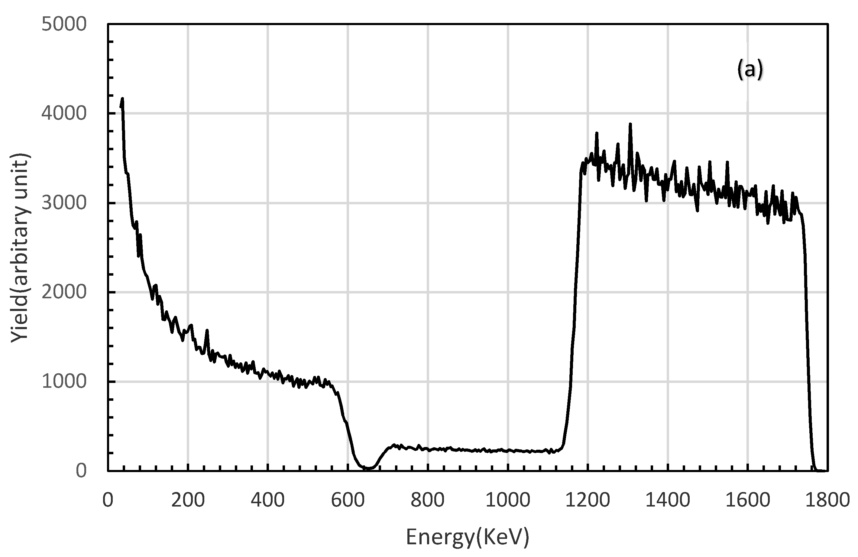
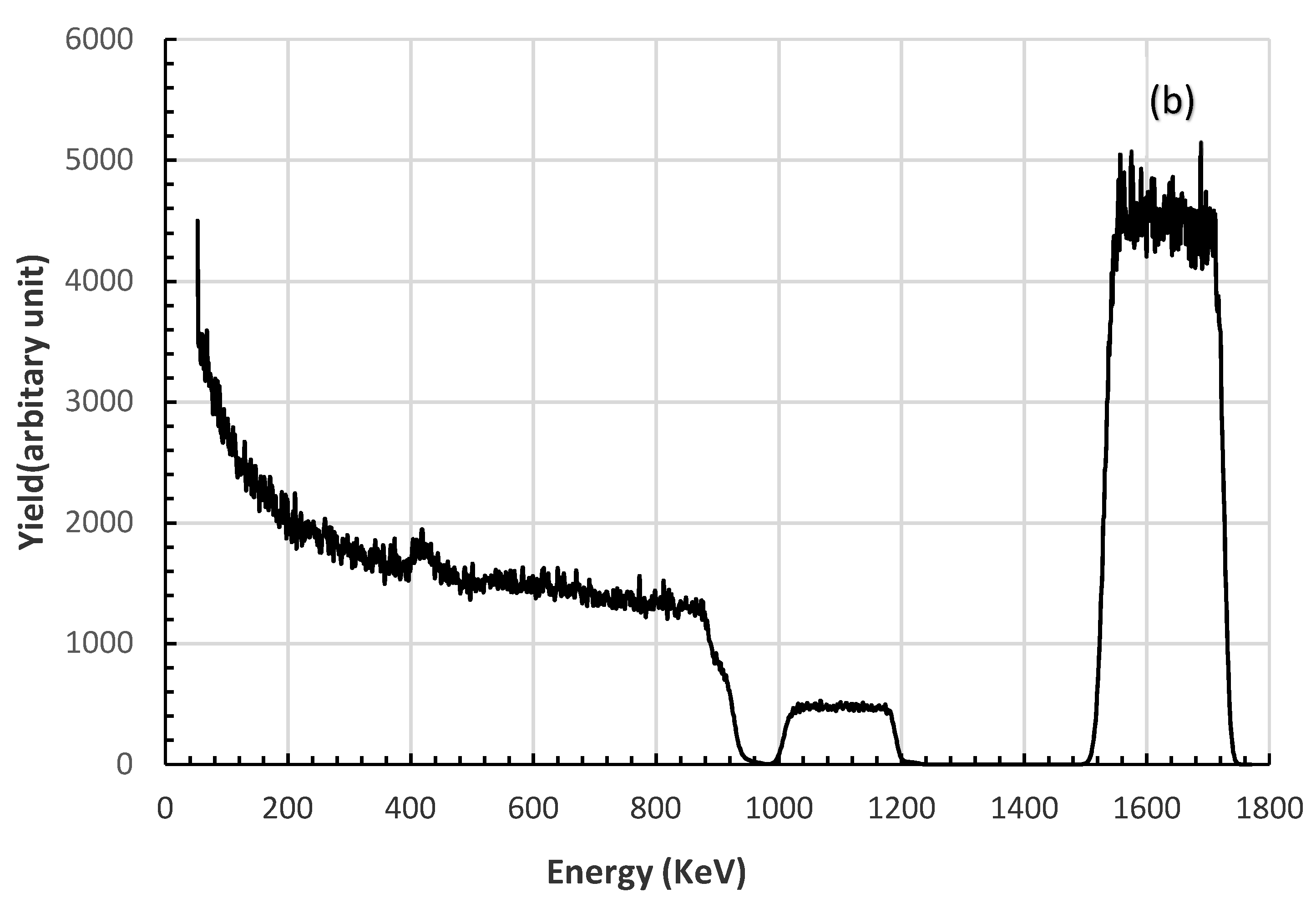
The proposed method and theoretical framework for solving the inverse problem in the spectral data analysis can be verified by numerical experiments. We have constructed a set of training and test data by utilizing a rigorous RBS spectrum simulation software package—SIMNRA 7.02 [39]. SIMNRA is a de facto standard simulation software for generating RBS spectra. It not only treats the basic scattering phenomena but also takes into account the subtle features in spectra that are arisen from complex interactions such as energy straggling effect, plural and multiple scattering, resonance, and surface roughness [39,40]. As an illustrative example, we consider a typical physical sample consisting of a film SnxS0.87−xO0.13 on the silicon substrate, where the structural parameters in this case include the thickness of the sample and concentration of Sn and S. The ion species in the simulated RBS spectra are alpha particles with the incident energy 2 MeV at a backscattering angle 165°. This is a typical experimental setting in RBS analysis. For the training purpose, the thickness and concentrations are randomly generated within the range between 400 × 1015 atoms/cm2 and 4000 × 1015 atoms/cm2, and between 0.32 and 0.55, respectively. The full data set used for the computer experiments is composed of a series of spectral curves (input vector), and the corresponding structural parameters (output vector). To make the synthetic spectra close to the realistic ones, Gaussian noises were added to the simulated smooth spectra. Figure 3a,b illustrate two typical simulation spectral curves and their corresponding structural parameters. Within the specific ranges of the sample thickness and concentrations, a total of 482 spectra are generated by running SIMNRA7.02. 75% of the full data is for training, and the remaining data is used for testing. It must mention that the pre-processing of spectroscopic data must be carried out since they vary in the different order of magnitudes. The pre-processing is made by applying a simple transformation zi = log10(zi + 10), which normalizes the spectral yield between 1 and 5. The spectral data are further compressed by the PAC method as described in Section 2.3, which produces a significant dimensional reduction. In this application, a spectral curve with 400 points, undergoing the dimensionality reduction by PCA, retains seven principal components (PCs) which sufficiently accounts for 99% variances in the dataset. Thus these principal components are selected as the new input variables for the constructed ELM network.
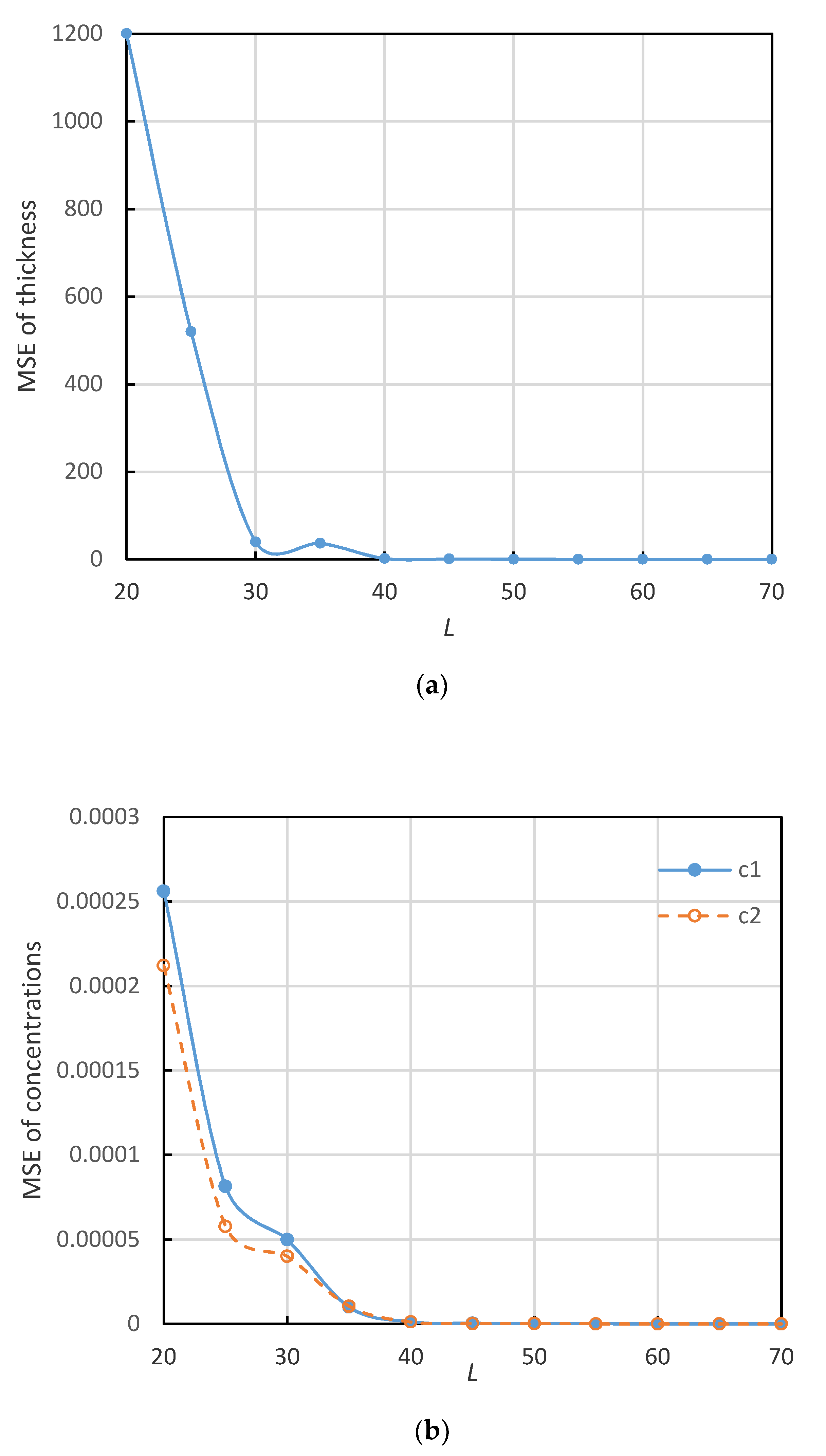
The numerical experiments are conducted under the MATLAB platform. The number of hidden layer node L is an adjustable parameter in the experiments. Some trials with different values of L have been tested. Figure 4a,b shows that the specified metrics—the mean squared errors (MSE) vary with L. It has been noted that MSEs, starting a large initial value, decrease quickly with the increase of the hidden layer node number and it tends to be stable to a non-zero minimal value when L takes values greater than 40, indicating a good convergence. The optimal number of L also could be available via an optimization method such as particle swarm optimization (PSO) where the MSE can be defined as the cost function.
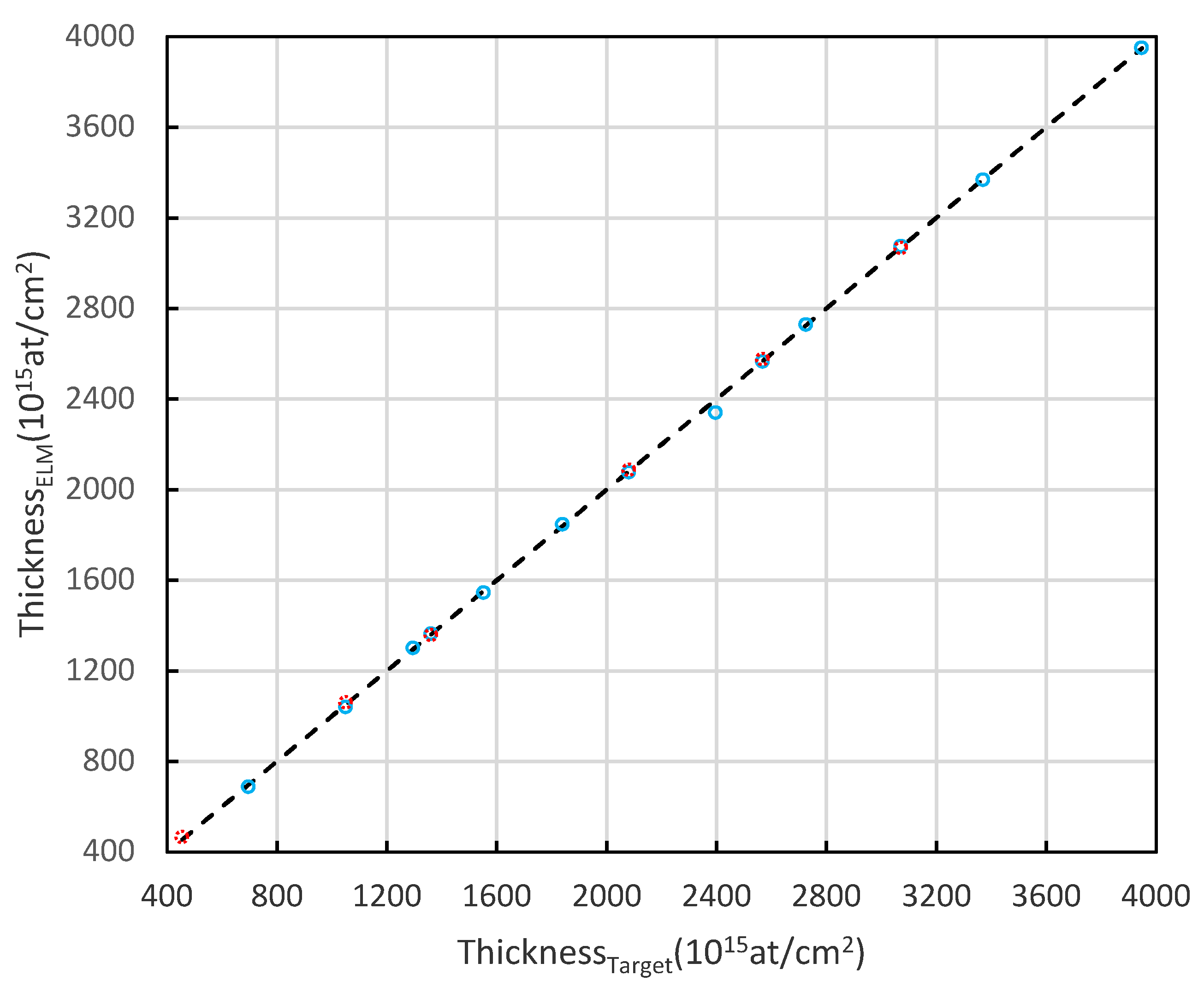
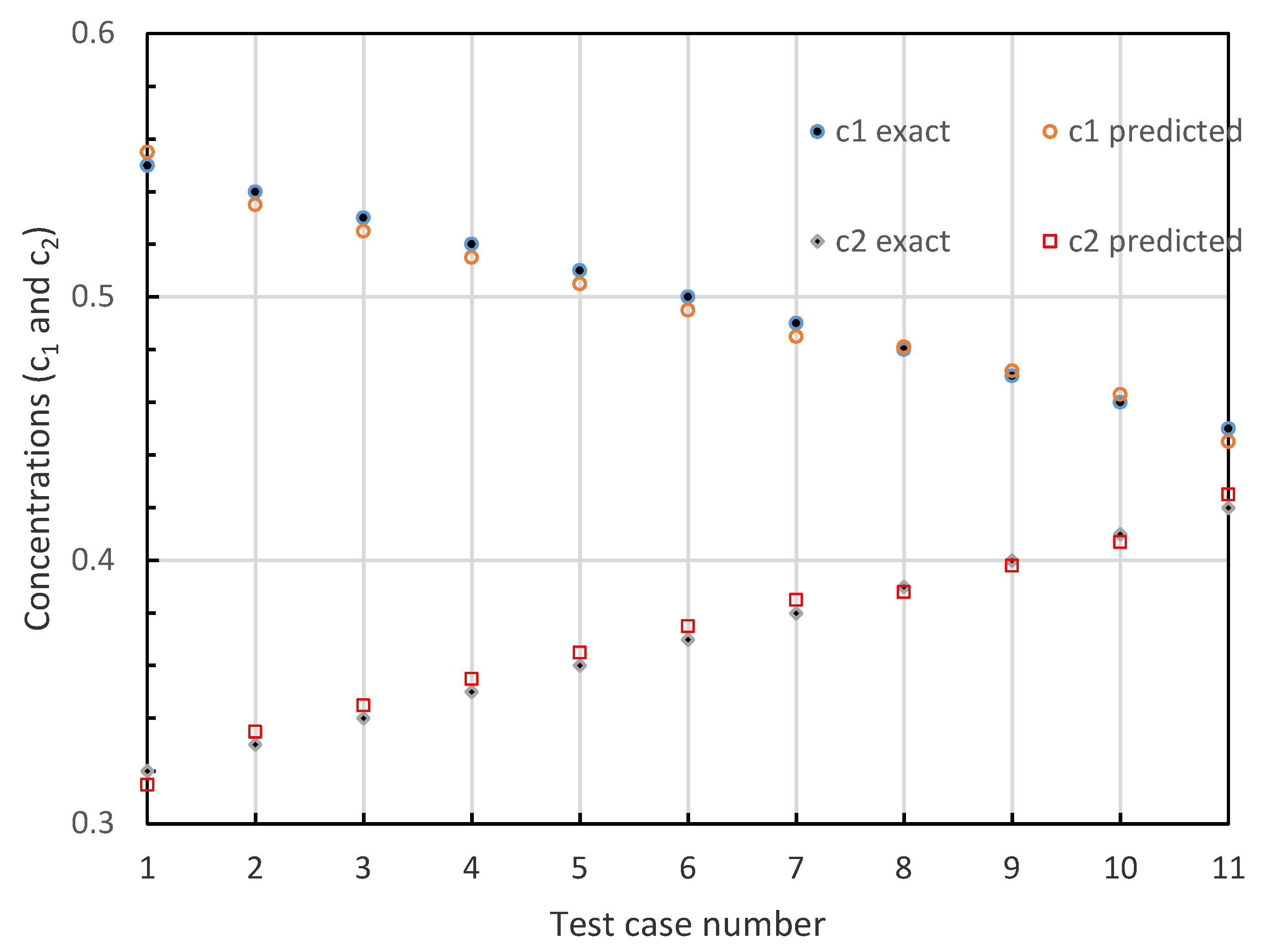
To further check the accuracy and the performance of the trained ELM network, it would be meaningful to examine the linear regression analysis of the output predictions on the test dataset. As shown in Figure 5 and Figure 6, the predictions of output results for selected cases by ELM accurately match the expected target values. Figure 5 illustrates that the ELM machine produces the accurate prediction values of the thickness variable, whereas Figure 6 shows the predictions of concentration variables with high accuracies.
After training and testing, the constructed ELM network can be used to analyze the spectral data with the unknown structural parameters of the samples by a generalization procedure. We select a few spectral curves to be analyzed and compare the predictions by the proposed ELM method with the results from calculations of a three-layer MLP network. The predicted outputs of both methods are summarized in Table 1 and Table 2. The ELM machine produces the correct analysis results for all cases with small errors. The maximum errors in the four sets of spectra for the thickness and concentrations are respectively 0.94%, 0.79%, and 0.97%. Compared to the ELM results with the exact nominal values of the structural parameter, it shows an excellent agreement. The maximum errors from the MLP method for the same test cases are 1.53%, 2.06%, and 2.54%, respectively. This comparison shows that the errors of MLP results are larger than ELM errors. For most numerical-based techniques, the analysis errors are typically around 5% [28]. It can be seen that ELM should be a better option for the applications in spectral data analysis. Unlike a deep neural network (for example, deep belief networks, and deep Boltzmann machines), the original ELM was established by a shallow architecture; however, it is still a very practical and valid method for resolving the problems of regression, classification, and recognition because of its architecture simplicity, high accuracy, and easy training [13]. The webpage of the reference [41] lists some benchmark examples and results that compare the performances of using ELM and deep neural networks (DNN) for the applications with datasets—MNIST OCR, 3D Shape Classification [42], and Traffic sign recognition [43]. It can be clearly seen that the training accuracies by ELM were better or equal to those by DNN, whereas the training time was shortened dramatically (less than in a few magnitude order).
4. Conclusions
A conceptual framework incorporating ELM and dimensionality reduction techniques for solving the inverse problem in spectral data analysis has been proposed in this article. The theoretical method is demonstrated by numerical experiments with simulated spectral data. The experimental results show that ELM networks can produce accurate output predictions for the input spectral curves, where the prior structural information of the physical sample is unknown. Spectral data analysis is a challenging job due to its property of non-uniqueness arisen from the solutions of the inverse problem. It heavily relies on much domain knowledge and technical expertise of the analysts. This work makes an original exploration of the possibilities of using a learning algorithm from available data to replace numerical intensive computing. The preliminary studies have demonstrated its accuracy and feasibility.
Our future work includes two aspects. First, the experimentally measured or simulated data from different types of spectroscopic techniques are required to be handled by a normalized method to accommodate various features from different type spectra so that a standard format of input data is established. Particularly, for complex emission spectra such as PIXE or gamma-ray analysis where the spectral peak width may be within a narrow energy region, more principal components are required to achieve an expected accuracy. Second, the proposed method can be implemented as application software that can be installed on a computer connecting to the real-time spectral data collecting system in the spectroscopy laboratory. Thus, an automated collection and intelligent analysis system can be integrated effectively. As the ELM method features a fast and near real-time learning process, it is possible to perform the real-time analysis for collecting batch spectral data with high accuracies. We believe that the data analysis method based on a learning algorithm rather than numerical intensive computations has a great potential to stimulate a conceptual breakthrough toward a pure data-driven spectroscopy analysis. This may promote industries to develop the new generation of automatic and general-use spectroscopy software based on machine learning algorithms.
Author Contributions
Conceptualization, M.L. and S.W.; Methodology, Software, Validation, M.L., S.W., W.L. and L.D.L.; Formal analysis, M.L. and S.W.; Investigation, Resources, M.L., S.W., W.L., and L.D.L.; Data curation, M.L.; Writing—original draft preparation, M.L.; Writing—review and editing, M.L., S.W., W.L., L.D.L.; Visualization, M.L. and L.D.L.; Supervision, M.L.; Project administration, M.L. and L.D.L.; Funding acquisition, M.L. and S.W. All authors have read and agreed to the published version of the manuscript.
Funding
This research received no external funding.
Acknowledgments
The authors would like to thank our colleague—Tim McSweeney for beneficial discussions and assistance. We also express our sincere gratitude to M. Mayer (Max-Plank Institute, Germany) for permission to use the trial version of the simulation software SIMNRA 7.02.
Conflicts of Interest
The authors declare no conflict of interest.
References
- Barradas, N.P.; Jeynes, C.; Webber, R.; Keissig, U.; Grotzschel, R. Unambiguous automatic evaluation of multiple ion beam analysis data with simulated annealing. Nucl. Instr. Meth. Phys. Res. B 1999, 149, 233–238. [Google Scholar] [CrossRef]
- van Laarhoven, P.J.M.; Aarts, E.H.L. Simulated Annealing. In Simulated Annealing: Theory and Applications. Mathematics and Its Applications; Springer: Berlin/Heidelberg, Germany, 1987; Volume 37. [Google Scholar]
- Orosz, J.; Jacobson, S. Analysis of Static Simulated Annealing Algorithms. J. Optim. Theory Appl. 2002, 115, 165–182. [Google Scholar] [CrossRef]
- Siddique, N.; Adeli, H. Simulated Annealing, Its Variants and Engineering Applications. Int. J. Artif. Intell. Tools 2016, 25, 1630001–1630025. [Google Scholar] [CrossRef]
- Barradas, N.; Vieira, A. Artificial neural network algorithm for analysis of Rutherford backscattering data. Phys. Rev. E 2000, 62, 5818–5829. [Google Scholar] [CrossRef] [PubMed]
- Demeulemeester, J.; Smeets, D.; Barradas, N.; Vieira, A.; Comrie, C.; Temst, K.; Vantomme, A. Artificial neural networks for instantaneous analysis of real-time Rutherford backscattering spectra. Nucl. Instr. Meth. Phys. Res. Sect. B Beam Interact. Mater. Atoms 2010, 268, 1676–1681. [Google Scholar] [CrossRef]
- Nene, N.R.; Vieira, A.; Barradas, N.P. Artificial neural networks analysis of RBS and ERDA spectra of multilayered multi-elemental samples. Nucl. Instr. Meth. Phys. Res. B 2006, 246, 471–478. [Google Scholar] [CrossRef]
- Wang, J.-S.; Chen, Y.-P. A fully automated recurrent neural network for unknown dynamic system identification and control. IEEE Trans. Circuits Syst. I Regul. Pap. 2006, 53, 1363–1372. [Google Scholar] [CrossRef]
- Bishop, C.M. Pattern Recognition and Machine Learning; Springer: New York, NY, USA, 2006. [Google Scholar]
- Lam, L.H.T.; Le, N.H.; Van Tuan, L.; Ban, H.T.; Hung, T.N.K.; Nguyen, N.T.K.; Dang, L.H.; Le, N.Q.K. Machine Learning Model for Identifying Antioxidant Proteins Using Features Calculated from Primary Sequences. Biology 2020, 9, 325. [Google Scholar] [CrossRef]
- Le, N.Q.K.; Do, D.T.; Chiu, F.-Y.; Yapp, E.K.Y.; Yeh, H.-Y.; Chen, C.-Y. XGBoost Improves Classification of MGMT Promoter Methylation Status in IDH1 Wildtype Glioblastoma. J. Pers. Med. 2020, 10, 128. [Google Scholar] [CrossRef]
- Deist, T.M.; Dankers, F.J.W.M.; Valdes, G.; Wijsman, R.; Hsu, I.; Oberije, C.; Lustberg, T.; Van Soest, J.; Hoebers, F.; Jochems, A.; et al. Machine learning algorithms for outcome prediction in (chemo)radiotherapy: An empirical comparison of classifiers. Med Phys. 2018, 45, 3449–3459. [Google Scholar] [CrossRef]
- Huang, G.-B.; Zhu, Q.-Y.; Siew, C.-K. Extreme learning machine: Theory and applications. Neurocomputing 2006, 70, 489–501. [Google Scholar] [CrossRef]
- Kasun, L.L.C.; Zhou, H.; Huang, G.B. Representational learning with ELMs for big data. IEEE Intell. Syst. 2013, 28, 31–34. [Google Scholar]
- Huang, G.-B. An Insight into Extreme Learning Machines: Random Neurons, Random Features and Kernels. Cogn. Comput. 2014, 6, 376–390. [Google Scholar] [CrossRef]
- Han, H.-G.; Wang, L.-D.; Qiao, J. Hierarchical extreme learning machine for feedforward neural network. Neurocomputing 2014, 128, 128–135. [Google Scholar] [CrossRef]
- Huang, G.-B.; Zhou, H.; Ding, X.; Zhang, R. Extreme Learning Machine for Regression and Multiclass Classification. IEEE Trans. Syst. Man Cybern. Part B 2012, 42, 513–529. [Google Scholar] [CrossRef] [Green Version]
- Huang, G.; Huang, G.B.; Song, S.; You, K. Trends in extreme learning machines: A review. Neural Netw. 2015, 61, 32–48. [Google Scholar] [CrossRef]
- Zheng, W.; Fu, X.; Ying, Y. Spectroscopy-based food classification with extreme learning machine. Chemom. Intell. Lab. Syst. 2014, 139, 42–47. [Google Scholar] [CrossRef]
- Zheng, W.; Shu, H.; Tang, H.; Zhang, H. Spectra data classification with kernel extreme learning machine. Chemom. Intell. Lab. Syst. 2019, 192. [Google Scholar] [CrossRef]
- da Costa, N.L.; Llobodanin, L.A.G.; de Lima, M.D.; Castro, I.A.; Barosa, R. Geographical recognition of Syrah wines by combining feature selection with extreme learning machine. Measurement 2018, 120, 92–99. [Google Scholar] [CrossRef]
- Quadram Institute. Available online: https://csr.quadram.ac.uk/example-datasets-for-download/ (accessed on 5 March 2020).
- Khan, B.; Wang, Z.; Han, F.; Iqbal, A.; Masood, R.J. Fabric weave pattern and yarn colour recognition and classification using a deep ELM network. Algorithms 2017, 10, 117. [Google Scholar] [CrossRef] [Green Version]
- Song, G.; Dai, Q.; Han, X.; Guo, L. Two novel ELM-based stacking deep models focused on image recognition. Appl. Intell. 2020, 50, 1345–1366. [Google Scholar] [CrossRef]
- Zhou, H.; Huang, G.-B.; Lin, Z.; Wang, H.; Soh, Y.C. Stacked Extreme Learning Machines. IEEE Trans. Cybern. 2015, 45, 2013–2025. [Google Scholar] [CrossRef]
- Tarantola, A. Inverse problem theory and methods for model parameter estimation. SIAM 2004. [Google Scholar] [CrossRef] [Green Version]
- Mosegaard, K.; Sambridge, M. Monte Carlo analysis of inverse problems. Inverse Probl. 2002, 18, R29–R54. [Google Scholar] [CrossRef]
- Kotai, E. Computer methods for analysis and simulation of RBS and ERDA spectra. Nucl. Instr. Meth. Phys. Res. B 1994, 85, 588–596. [Google Scholar] [CrossRef]
- Denison, D.G.T.; Mallick, B.K.; Smith, A.F.M. Automatic Bayesian curve fitting. J. R. Stat. Soc. Ser. B 1998, 60, 333–350. [Google Scholar] [CrossRef]
- Hastie, T.; Tibshirani, R.; Friedman, J.H. The Elements of Statistical Learning: Data Mining, Inference, and Prediction, 2nd ed.; Springer Series in Statistics; Springer: New York, NY, USA, 2009. [Google Scholar]
- Broomhead, D.S.; Lowe, D. Multivariable function interpolation and adaptive networks. Complex Syst. 1998, 2, 321–355. [Google Scholar]
- Park, J.; Sandberg, I.W. Universal Approximation Using Radial-Basis-Function Networks. Neural Comput. 1991, 3, 246–257. [Google Scholar] [CrossRef] [PubMed]
- Li, M.; Li, L.D. A Novel Method of Curve Fitting Based on Optimized Extreme Learning Machine. Appl. Artif. Intell. 2020, 34, 849–865. [Google Scholar] [CrossRef]
- Li, M.; Wibowo, S.; Guo, W. Nonlinear Curve Fitting Using Extreme Learning Machines and Radial Basis Function Networks. Comput. Sci. Eng. 2019, 21, 6–15. [Google Scholar] [CrossRef]
- Serre, D. Matrices: Theory and Applications; Springer: New York, NY, USA, 2002. [Google Scholar]
- Haykin, S. Neural Networks: A Comprehensive Foundation, 3rd ed.; Pearson: London, UK, 2009. [Google Scholar]
- Serneels, S.; Verdonck, T. Principal component analysis for data containing outliers and missing elements. Comput. Stat. Data Anal. 2008, 52, 1712–1727. [Google Scholar] [CrossRef]
- Belsley, D.A.; Kuh, E.; Welsch, R.E. Regression Diagnostics. Identifying Influential Data and Sources of Collinearity; Wiley: New York, NY, USA, 1980. [Google Scholar]
- Mayer, M. SIMNRA 7.02 User’s Guide. Max-Planck Institute of Plasma Physics; Max-Planck-Institut für Plasmaphysik: Garching, Germany, 2019. [Google Scholar]
- Mayer, M. Improved Physics in SIMNRA 7. Nucl. Instr. Meth. Phys. Res. B 2014, 332, 176–187. [Google Scholar] [CrossRef]
- Extreme Learning Machines (ELM). Extreme Learning Machines (ELM): Filling the Gap between Frank Rosenblatt’s Dream and John von Neumann’s Puzzle. Available online: https://www.ntu.edu.sg/home/egbhuang/ (accessed on 5 March 2020).
- Xie, Z.; Xu, K.; Shan, W.; Liu, L.; Xiong, Y.; Huang, H. Projective Feature Learning for 3D Shapes with Multi-View Depth Images. Comput. Graph. Forum 2015, 34, 1–11. [Google Scholar] [CrossRef]
- Aziz, S.; Mohamed, E.A.; Youssef, F. Traffic Sign Recognition Based On Multi-feature Fusion and ELM Classifier. Procedia Comput. Sci. 2018, 127, 146–153. [Google Scholar] [CrossRef]
Figure 1.
Rutherford backscattering spectroscopy (RBS) backscattering process and the definition of the inverse problem.
Figure 1.
Rutherford backscattering spectroscopy (RBS) backscattering process and the definition of the inverse problem.

Figure 2.
The extreme learning machine (ELM) architecture diagram for the current RBS data analysis problem.
Figure 2.
The extreme learning machine (ELM) architecture diagram for the current RBS data analysis problem.
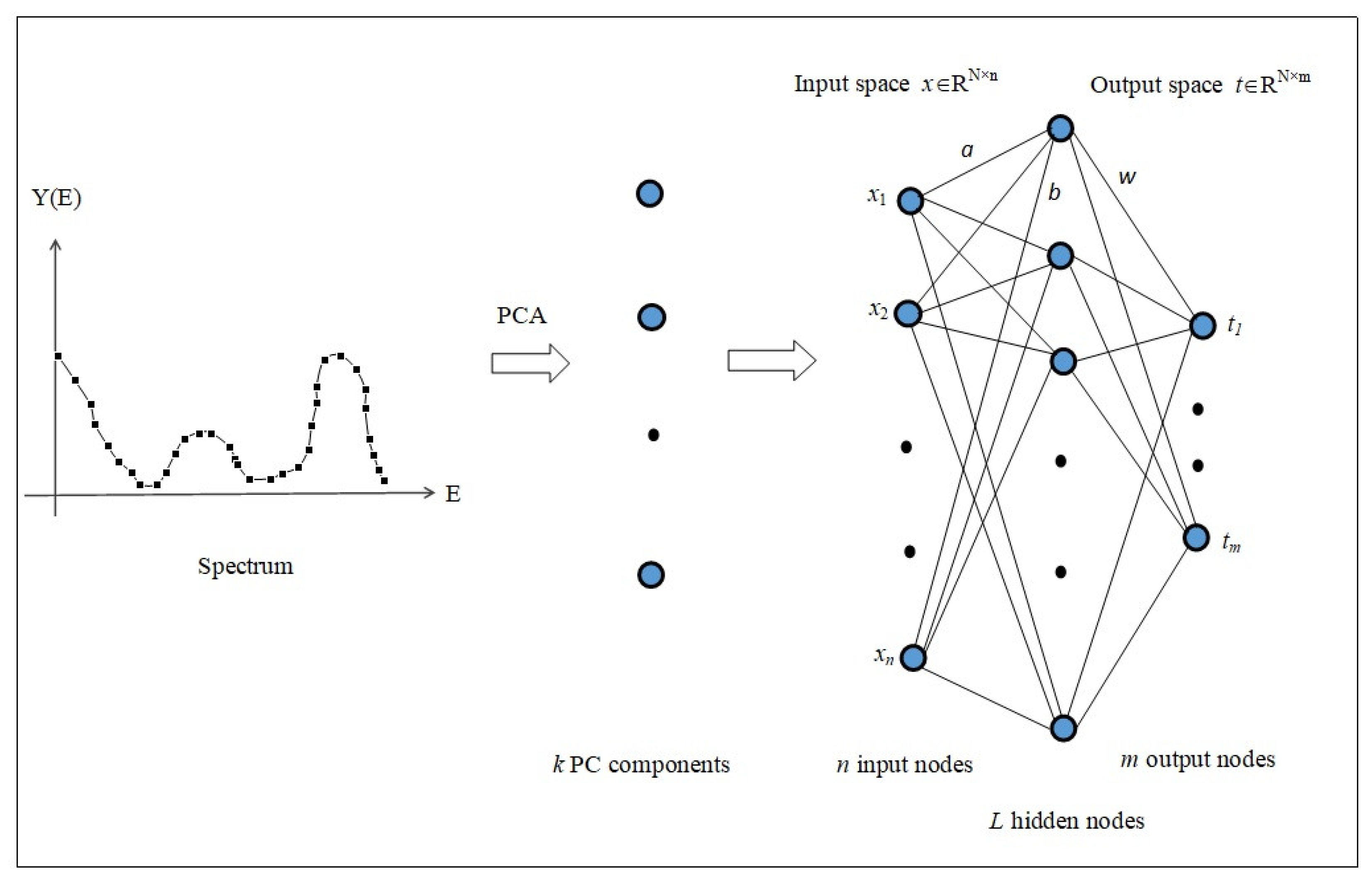
Figure 3.
Two representative RBS spectra in the training dataset and their corresponding structural parameters of the physical samples (a) t = 3641.19 × 1015 atoms/cm2, c1 = 0.5105, c2 = 0.3595 (b) t = 1361.46 × 1015 atoms/cm2, c1 = 0.4417, c2 = 0.4283.
Figure 3.
Two representative RBS spectra in the training dataset and their corresponding structural parameters of the physical samples (a) t = 3641.19 × 1015 atoms/cm2, c1 = 0.5105, c2 = 0.3595 (b) t = 1361.46 × 1015 atoms/cm2, c1 = 0.4417, c2 = 0.4283.


Figure 4.
(a). The mean squared errors (MSE) of the thickness variation with L (the number of hidden layer nodes). (b). The MSE of the concentrations of c1, c2 variation with L (the number of hidden nodes).
Figure 4.
(a). The mean squared errors (MSE) of the thickness variation with L (the number of hidden layer nodes). (b). The MSE of the concentrations of c1, c2 variation with L (the number of hidden nodes).

Figure 5.
The ELM predicted thickness vs. exact target values.

Figure 6.
The ELM predicted concentrations vs. exact target values.


Table 1.
ELM predicted results and exact values.
| Sample No | Exact Values | ELM Predictions | ||||
|---|---|---|---|---|---|---|
| t × 1015 at/cm2 | c1 | c2 | t × 1015 at/cm2 | c1 | c2 | |
| 1 | 697.82 | 0.5400 | 0.3300 | 704.37 | 0.5389 | 0.3311 |
| 2 | 1295.88 | 0.5100 | 0.3600 | 1302.48 | 0.5111 | 0.3589 |
| 3 | 2397.33 | 0.4800 | 0.3900 | 2413.15 | 0.4762 | 0.3938 |
| 4 | 3072.98 | 0.4500 | 0.4200 | 3065.29 | 0.4484 | 0.4216 |
Table 2.
Multilayer perceptron (MLP) predicted results and exact values.
| Sample No | Exact Values | MLP Predictions | ||||
|---|---|---|---|---|---|---|
| t × 1015 at/cm2 | c1 | c2 | t × 1015 at/cm2 | c1 | c2 | |
| 1 | 697.82 | 0.5400 | 0.3300 | 708.55 | 0.5366 | 0.3334 |
| 2 | 1295.88 | 0.5100 | 0.3600 | 1290.33 | 0.5134 | 0.3566 |
| 3 | 2397.33 | 0.4800 | 0.3900 | 2422.32 | 0.4701 | 0.3998 |
| 4 | 3072.98 | 0.4500 | 0.4200 | 3088.52 | 0.4454 | 0.4246 |
Publisher’s Note: MDPI stays neutral with regard to jurisdictional claims in published maps and institutional affiliations. |
© 2021 by the authors. Licensee MDPI, Basel, Switzerland. This article is an open access article distributed under the terms and conditions of the Creative Commons Attribution (CC BY) license (http://creativecommons.org/licenses/by/4.0/).
Share and Cite
MDPI and ACS Style
Li, M.; Wibowo, S.; Li, W.; Li, L.D. Quantitative Spectral Data Analysis Using Extreme Learning Machines Algorithm Incorporated with PCA. Algorithms 2021, 14, 18. https://0-doi-org.brum.beds.ac.uk/10.3390/a14010018
AMA Style
Li M, Wibowo S, Li W, Li LD. Quantitative Spectral Data Analysis Using Extreme Learning Machines Algorithm Incorporated with PCA. Algorithms. 2021; 14(1):18. https://0-doi-org.brum.beds.ac.uk/10.3390/a14010018
Chicago/Turabian StyleLi, Michael, Santoso Wibowo, Wei Li, and Lily D. Li. 2021. "Quantitative Spectral Data Analysis Using Extreme Learning Machines Algorithm Incorporated with PCA" Algorithms 14, no. 1: 18. https://0-doi-org.brum.beds.ac.uk/10.3390/a14010018
Note that from the first issue of 2016, this journal uses article numbers instead of page numbers. See further details here.