Advanced Construction of the Dynamic Matrix in Numerically Efficient Fuzzy MPC Algorithms


Institute of Control and Computation Engineering, Warsaw University of Technology, Nowowiejska 15/19, 00-665 Warszawa, Poland
Algorithms 2021, 14(1), 25; https://0-doi-org.brum.beds.ac.uk/10.3390/a14010025
Submission received: 7 December 2020
/
Revised: 13 January 2021
/
Accepted: 14 January 2021
/
Published: 17 January 2021
(This article belongs to the Special Issue Model Predictive Control: Algorithms and Applications)
Abstract
:A method for the advanced construction of the dynamic matrix for Model Predictive Control (MPC) algorithms with linearization is proposed in the paper. It extends numerically efficient fuzzy algorithms utilizing skillful linearization. The algorithms combine the control performance offered by the MPC algorithms with nonlinear optimization (NMPC algorithms) with the numerical efficiency of the MPC algorithms based on linear models in which the optimization problem is a standard, easy-to-solve, quadratic programming problem with linear constraints. In the researched algorithms, the free response obtained using a nonlinear process model and the future trajectory of the control signals is used to construct an advanced dynamic matrix utilizing the easy-to-obtain fuzzy model. This leads to obtaining very good prediction and control quality very close to those offered by NMPC algorithms. The proposed approach is tested in the control system of a nonlinear chemical control plant—a CSTR reactor with the van de Vusse reaction.
1. Introduction
The Model Predictive Control (MPC) algorithms use the model of the control plant to predict the behavior of the process. Thanks to such an approach, the MPC algorithms can be successfully applied in control systems of processes with delays, with the inverse response, with constraints, and for MIMO (Multiple-Input Multiple-Output) processes; see, e.g., [1,2,3,4,5,6,7,8,9,10,11]. This is because the future control signal trajectories are generated by the MPC algorithms in such a way that the predicted, many sampling instants ahead, future behavior of the control plant and the shape of control signals fulfill the assumed criteria. Thus, the optimization problem, solved in each time step of the MPC algorithm to obtain these control signal trajectories, has the following form [1,4,7,9,12]:
subject to:
where:
where denotes a value, predicted using a process model the MPC algorithm is based on, of the jth output for the th sampling instant from the prediction horizon, derived at the kth sampling instant, and is an element of the reference trajectory for the jth output and for the th sampling instant from the prediction horizon; if reference trajectories constant on the prediction horizon are used, then:
where denotes a setpoint value for the jth output; are the decision variables of the optimization problem, being future changes in manipulated variables; contains p elements, and denote the weighting coefficients for the predicted control errors of the jth output; contains s elements, and denote the weighting coefficients for the changes of the mth manipulated variable; p is the prediction horizon; s is the control horizon; is the number of output variables; is the number of manipulated variables; , denote the vectors defining the lower and upper bounds of the changes of the control signals; , denote vectors defining the lower and upper bounds of the values of the control signals; and , denote the vectors defining the lower and upper bounds of the values of the output variables.
The optimization problem (1)–(4) is formulated and solved in each sampling instant, yielding the optimal vector of future control action. From the vector , the elements are extracted and applied in the control system. Then, the described procedure is repeated in the next time step.
1.1. MPC Algorithms Based on Linear Models
The simplest MPC algorithms are based on linear process models; see, e.g., [1,13]. In such a case, the superposition principle holds; therefore, the vector of predicted output values can be decomposed into two parts:
where is called the free response of the control plant describing the influence of the past values of control signals on the process and is called the forced response, depending on the future changes of the control signals ; the matrix is called the dynamic matrix and has the following form:
where denote the step response coefficients of the control plant, describing the influence of the mth control on the jth output; for details, see, e.g., [9].
After applying the prediction based on a linear model (12), the performance function (1) is transformed into a function that depends quadratically on the decision variables :
The prediction (12) depends linearly on the decision variables; therefore, after using it in the constraints on the output values (4), the optimization problem (1)–(4) becomes an easy-to-solve, standard quadratic optimization problem, with linear constraints. Unfortunately, the control performance offered by an LMPC algorithm, applied to a nonlinear process, may be unsatisfactory. In order to improve it, one can use an MPC algorithm based on a nonlinear model.
1.2. MPC Algorithms Based on Nonlinear Models
Assume that we have a nonlinear process model:
where is a vector that contains output values measured at the th sampling instant and is a vector that contains control values applied at the th sampling instant; denote the output values generated by the model in the th sampling instant as ; determine how many past output and control values the model needs. If one wants to use the model (17) directly in the optimization problem (1)–(4), then the prediction takes the form of the following formulas, passed to the optimization problem as a set of equality constraints:
where is a vector containing future control values, depending on the decision variables from the vector and:
where is a vector of recently measured output values; it is assumed that is the same for all instants in the prediction horizon—an approach proposed in the Dynamic Matrix Control (DMC) algorithm and therefore called the DMC-type disturbance model; see, e.g., [9].
Unfortunately, the optimization problem (1)–(4) with the prediction (18), based on a nonlinear model, is, in general, a non-convex nonlinear optimization problem; see, e.g., [14,15,16]. Thus, it is a hard-to-solve, time-consuming computational task, and there is no guarantee of finding a global solution, while the time needed to obtain the solution cannot be foreseen in advance. One of the methods to overcome this problem is to use so-called fast NMPC algorithms in which a suboptimal solution is generated faster than in the standard approach; see, e.g., [17,18,19]. To this group of methods belongs also the explicit approach in which most of the calculations are done off-line; see, e.g., [20,21,22] (it is interesting that this approach is optimal if the linear model is used [23,24,25]). Unfortunately, in this approach, the complexity of the controller grows significantly with the number of constraints taken into consideration.
If the process behavior is described by means of a fuzzy model, then the standard NMPC approach can be used, but also the structure of the model can be exploited to formulate algorithms that are easier to solve. One group of such algorithms is based on Linear Matrix Inequalities (LMIs); see, e.g., [26,27,28,29,30]. The other group is based on the classical fuzzy Takagi–Sugeno approach in which a few algorithms in the form of control laws, based on linear models, are used to obtain the fuzzy controller; see, e.g., [31,32].
In the other method, the linearization of the process model for the MPC algorithm is obtained in each time step, and the linear prediction relative to control changes is formulated; see, e.g., [9,33,34,35,36,37,38,39]. As a result, the optimization problem solved by the MPC algorithm in each time step is formulated as the quadratic one (like in LMPC algorithms). In the linearization-based algorithms, the prediction can be based on a classical linearization or a method of prediction generation can exploit the structure of the nonlinear model on which it is based. In the algorithms using the fuzzy Takagi–Sugeno model, described in [36,39], both the free response and the dynamic matrix are obtained using the model obtained after the linearization. In the algorithms detailed in [33,37], the (classical) free response is calculated using the nonlinear model. In [12], the advanced free response, calculated using the nonlinear model (which can have any form of the model generating outputs on the basis of input signals), takes into consideration the previously calculated trajectory of the future control signals (it can be improved iteratively if needed; the approach is similar, though slightly different in details, to the iterative prediction improvement in the iterative learning-based approaches to batch control described in [40,41,42]); the dynamic matrix is generated using the easy-to-obtain fuzzy model.
The approach proposed in the article is an extension of the algorithms presented in [12]. It is done in such a way that the optimization problem solved by the MPC algorithm in each time step is the quadratic one. The modification is introduced in the method of dynamic matrix construction. In [12], elements in the dynamic matrix were obtained taking into consideration the current operation point. Changes of the operating point on the prediction horizon are taken into consideration in the proposed approach. This is done using the free response, generated using the nonlinear control plant model. The obtained prediction is, however, still linear with respect to control changes. Thus, the algorithms utilizing the proposed approach combine the computational simplicity of the LMPC algorithms with the control performance offered by the NMPC algorithms.
The next section details the formulation of the Fuzzy MPC (FMPC) algorithms based on fuzzy and nonlinear models, with the advanced construction of the dynamic matrix. In Section 3, the operation of the FMPC algorithms exploiting the proposed advanced dynamic matrix is tested in a simulation example of the control system of a nonlinear chemical reactor with the inverse response. Conclusions are presented in the last section.
2. Efficient Fuzzy MPC Algorithms with the Advanced Construction of the Dynamic Matrix
The complications resulting from the need to solve a nonlinear optimization task by the MPC algorithm in each time step can be avoided by using an approximation of the process model carried out in each time step. Then, a nonlinear model is used to obtain the free response in such a way that the prediction is linear relative to decision variables, but mimics the nonlinearity of the process very well. An easy-to-obtain fuzzy model is used to get the dynamic matrix.
The dynamic matrix can be constructed in different ways. In Section 2.2, it is described how to do it in such a way that it fits the nonlinearity of the process better than in the standard approach. The method is based on a skillful utilization of the free response (generated using the nonlinear process model). Then, using both elements needed to obtain the prediction, the free response and the dynamic matrix, the optimization problem (1)–(4), solved in each time step, is formulated as a quadratic optimization problem. Such a problem is easy to solve using commonly available optimization routines. Moreover, the simplified versions of the algorithms, in which a control law is obtained, are also discussed.
The proposed algorithms are the generalization of their counterparts proposed in [12]. They use the same free response generation (reminded in Section 2.1) and the same formulation of the optimization problems solved at each time step (reminded in Section 2.3). The difference is in the way the dynamic matrix is constructed (the topic detailed in Section 2.2.3).
2.1. Generation of the Free Response
The method of advanced free response generation, based on a nonlinear process model, proposed in [12], is reminded in this subsection. Define the following vectors:
where are elements of control signal trajectories obtained in the last st time step.
First, the components of the free response are derived iteratively using the nonlinear model (17) and the vectors (20):
Note that the values are used when calculating the output values , and in general, in the ith iteration, the values are used to obtain .
Next, the final form of the free response is obtained, after taking into account the estimation of unmeasured disturbances :
2.2. Generation of the Dynamic Matrix
2.2.1. Fuzzy Model Used to Obtain the Dynamic Matrix
The fuzzy Takagi–Sugeno model used to generate the dynamic matrix has the following form:
where is the value of the th output variable at the th sampling instant, is the value of th manipulated variable at the th sampling instant, , are fuzzy sets, are the coefficients of step responses in the fth local model, , , and l is number of fuzzy rules. The model is composed of local models in the form of step responses [39]; thus, it can be obtained relatively easily, because it is sufficient to collect a few sets of step responses, near a few operating points, e.g., using a nonlinear model of the process. Next, the premises of the model should be formulated using expert knowledge and then tuned, e.g., by means of a fuzzy neural network [9].
2.2.2. Standard Dynamic Matrix
In order to calculate the output values of the model (23), the normalized firing strengths of the fuzzy rules should be calculated using fuzzy reasoning; see, e.g., [44,45]. These values are calculated using the previous values of the output and control signals. In the kth sampling instant, the normalized firing strengths are obtained, then the output values of the model are as follows:
where:
In the standard approach to the dynamic matrix generation, exploited, e.g., in [12,46,47], the parameters are used in the construction of the dynamic matrix in the same way as in the LMPC algorithm, i.e., they are used at each sampling instant from the prediction horizon despite being calculated using the firing strengths obtained in the current (kth) sampling instant. Thus, they are obtained for the current operating point, which in general, changes on the prediction horizon. Therefore, now the improved version of the dynamic matrix, adopting the nonlinearity of the process on the prediction horizon, will be proposed. It can be relatively easily obtained using the elements of the free response and of the trajectory of future control signals. The method is detailed below.
2.2.3. Advanced Dynamic Matrix Generation
In the first time step from the prediction horizon, the fuzzy model (generating outputs for the st time step) has the following form:
However, are not known yet, but the approach used in the free response generation can be applied here, i.e., the appropriate element of the future trajectory of the control signals can be used, namely: . Therefore, the premises used to obtain the firing strengths of the fuzzy rules will be as follows:
As a result, the normalized firing strengths of the fuzzy rules will be obtained for the time step from the prediction horizon (calculated at the kth sampling instant, using the fuzzy reasoning); the appropriate elements of the dynamic matrix will be then calculated using the formula:
In the second time step from the prediction horizon, the fuzzy model has the following form:
This time, however, not only are not known yet, but also and . One can use the approach from the previous step, i.e., instead of , is used. The other problem is that also the values are not known yet. However, one can use the appropriate elements of the free response here, namely . Therefore, the premises used to obtain the firing strengths in the next nd time step from the prediction horizon will have the following form:
the normalized firing strengths , obtained for the nd time step from the prediction horizon, using (30), are then utilized to calculate the elements of the dynamic matrix corresponding to the nd time step from the prediction horizon:
This procedure is repeated iteratively in the next time steps from the prediction horizon, resulting in obtaining the normalized firing strengths of the fuzzy rules in each, th, time step from the prediction horizon. Next, the appropriate elements of the dynamic matrix, for each th time step from the prediction horizon, will be calculated using the formula:
Now, the dynamic matrix can be generated (and updated in each sampling instant):
Note that in the ith row of each matrix , the elements calculated for the th time step from the prediction horizon are used.
Assume that the firing strengths for a given fuzzy rule are grouped in the following vector:
and define:
Then, the matrices can be calculated using the relatively simple formula:
where is the identity matrix of dimension , and the matrices remain the same in each time step.
2.3. Optimization Problem in the Numerical and Analytical Versions of the Algorithms
Now, assume that future control values are decomposed as follows:
where can be interpreted as the corrections of the control signal obtained in the last st time step. Thus, future control increments are described by the following, similar formula:
Note that the values and are known, as they were calculated in the last time step, and their influence on the output variables is contained in the free response (22), described in Section 2.1. Therefore, now the dynamic matrix (33) will be used to predict the influence of control corrections on the control plant outputs, and after using the free response (22) and the dynamic matrix (33), one obtains the following prediction:
where:
Note that the prediction depends linearly on corrections .
2.3.1. Optimization with the Classical Performance Index
Optimization task (1)–(4), which is solved by the control algorithm in each time step, changes now to the following form with corrections being the decision variables:
subject to:
where , , and:
contain elements of the future control increments’ trajectory and of the future control trajectory.
Note that the performance function in (42) depends quadratically on decision variables , and all constraints depend linearly on decision variables. Thus, a standard, easy-to-solve linear-quadratic optimization problem is obtained.
If in each time step, the optimization problem with performance function from (42) is solved without constraints, then it has the following solution given by the analytical formula:
2.3.2. Optimization with the Modified Performance Index
The change consists of the modification of the second component of the performance index, which now depends only on the corrections of the control signals . This modification leads to algorithms that generate faster responses, but the influence of the parameter on system robustness becomes significantly limited.
If the performance index (47) is minimized without constraints, then the following analytical solution is obtained:
2.3.3. Utilization of Analytical Versions of the Algorithms
Due to the fact that the dynamic matrix changes, in general, in every time step, then in each time step, the formula (46) or (48) allowing calculating the control action should be used by the algorithm. As a consequence, appropriate rows of the matrix (corresponding to the control increments for the current sampling instant ) should be calculated by the algorithm in each time step.
3. Example
3.1. Control Plant
The control plant is a nonlinear, isothermal CSTR in which the van de Vusse reaction takes place. These CSTRs are a popular benchmark due to their nonlinearity and difficult dynamics, willingly used to test newly developed control algorithms; see, e.g., [48,49,50,51,52,53]. The process model of the reactor is composed of two composition balance equations; see, e.g., [54]:
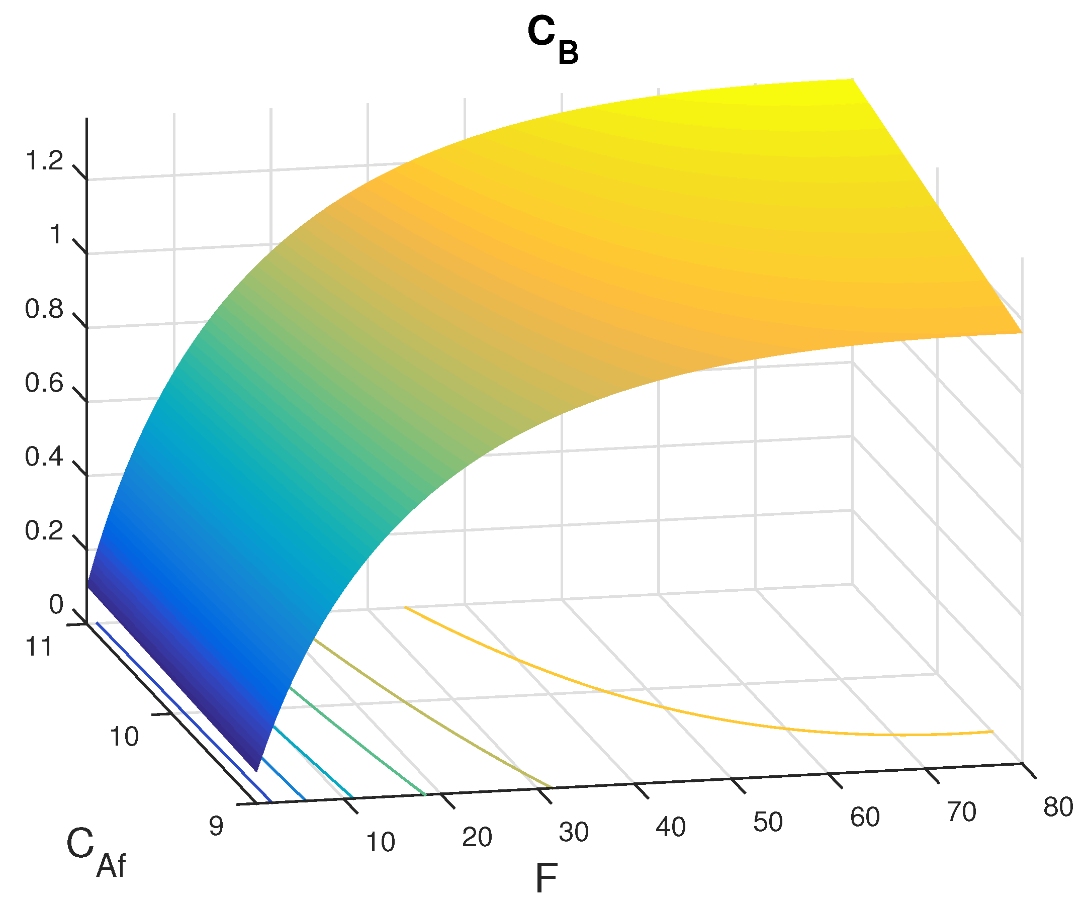
where , are the concentrations of Components A and B, respectively, F is the inlet (and also outlet) flow rate, V is the volume in which the reaction takes place (assumed constant and ), and is the concentration of Component A in the inlet flow stream (if not declared otherwise, it is assumed that ). The values of the parameters are: , , . The output variable is the concentration of Substance B. The manipulated variable is the inlet flow rate F. is the disturbance variable.
The described control plant was used during the tests also in [12]. Its nonlinear steady-state characteristic is reminded in Figure 1. The control plant has the inverse response; thus, it is natural to use an MPC algorithm in this case.
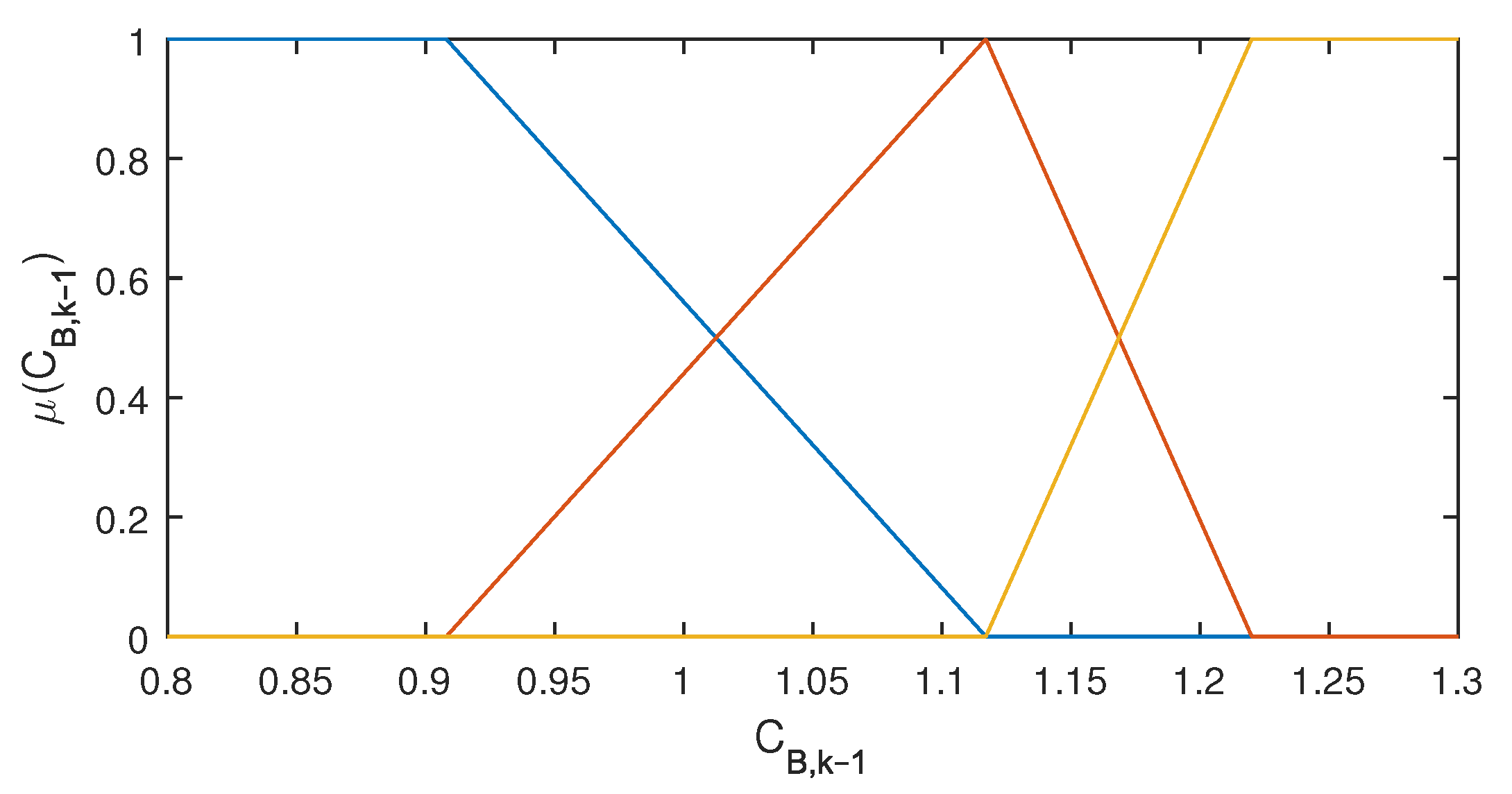
The fuzzy model used to generate the dynamic matrix, in the researched algorithms, is the same as in [12]. It is composed of three step responses obtained near the following operating points:
- R1 0.91 mol/L, 2.18 mol/L, 20 L/h;
- R2 1.12 mol/L, 3 mol/L, 34.3 L/h;
- R3 1.22 mol/L, 3.66 mol/L, 50 L/h.
The assumed membership functions are reminded in Figure 2.
3.2. Experiments
For the considered control plant, a few MPC algorithms were designed:
- -
- NMPC—based on the nonlinear model and nonlinear optimization and numerically efficient FMPC algorithms with advanced free response generation, proposed in [12], and:
- -
- FMPC1 with the conventional dynamic matrix and the classical performance index,
- -
- FMPC2 with the conventional dynamic matrix and the modified performance index,
- -
- FMPC1a with the advanced dynamic matrix and the classical performance index,
- -
- FMPC2a with the advanced dynamic matrix and the modified performance index.
The simulation experiments were done using MATLAB. During the experiments, the operation of the control systems with the NMPC and FMPC algorithms was compared. The FMPC algorithms use the nonlinear model in the form of state equations, to generate the free response and the fuzzy model (23) to obtain the dynamic matrix. A sampling time equal to s was assumed; the values of tuning parameters were as follows (if not declared otherwise): prediction horizon , control horizon , and weighting coefficient .
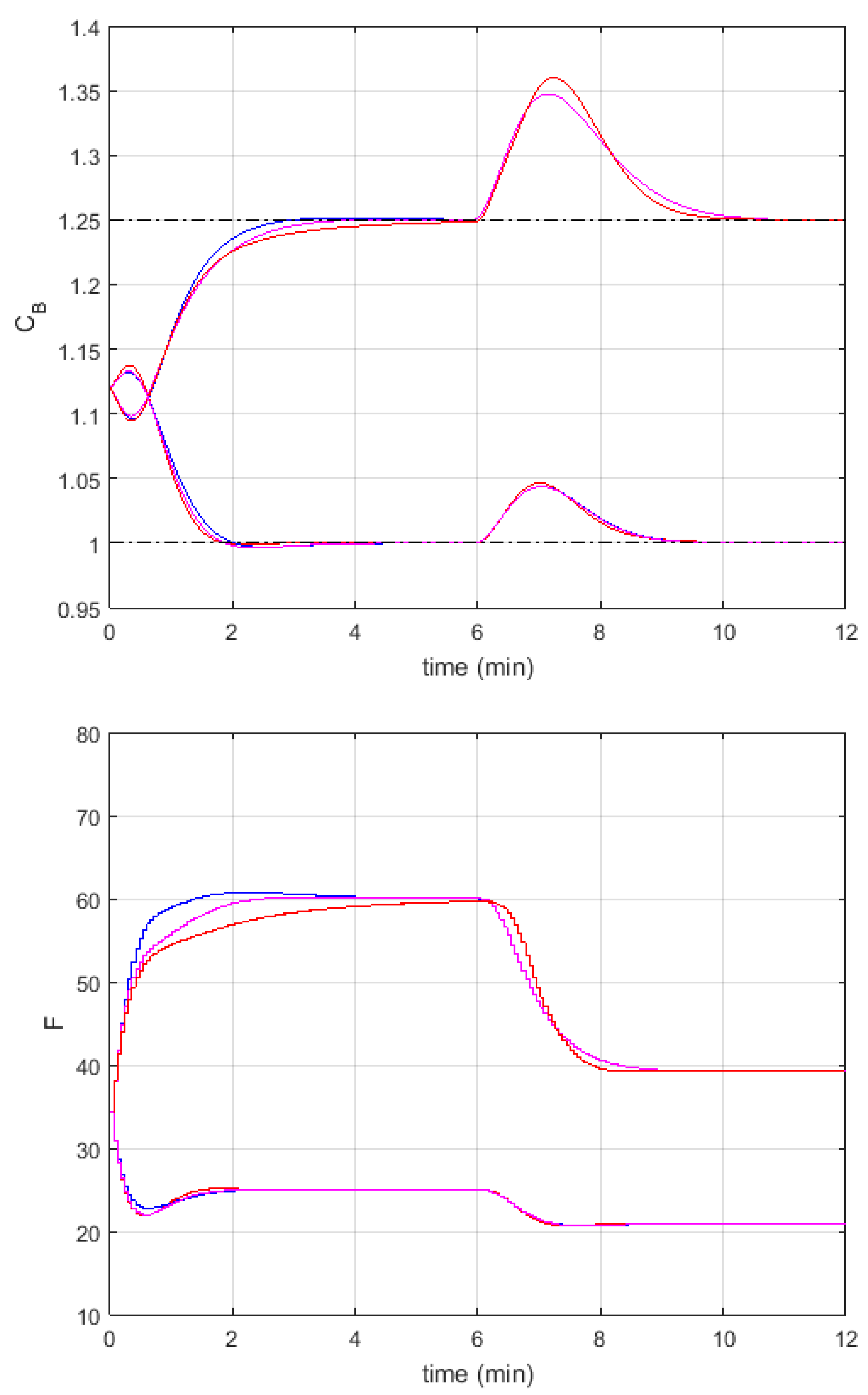
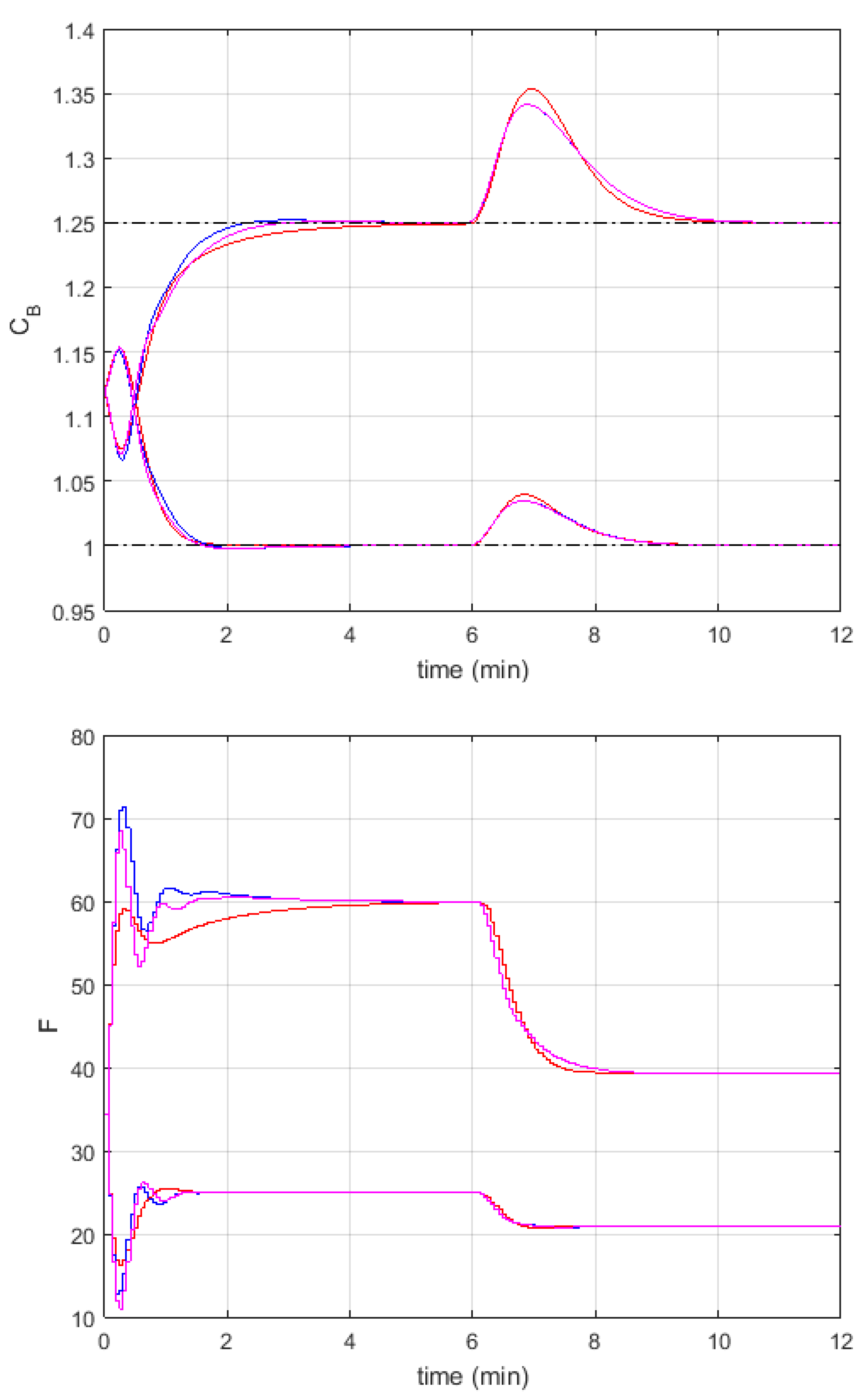
The responses of the control systems to changes in the setpoint and to the change of the disturbance by 10% in the 6th minute of the experiment are shown in Figure 3 and Figure 4. If the setpoint was changed to mol/L, the responses obtained in the control system with the FMPC1a algorithm (magenta lines in Figure 3) and with the FMPC1 algorithm (blue lines in Figure 3) were very close to those obtained with the NMPC algorithm with nonlinear optimization (red lines in Figure 3). In all cases, there was almost no overshoot. The FMPC algorithms were slightly faster than the NMPC algorithm.
In the case when the setpoint changed to mol/L, the response obtained with the FMPC1 algorithm was the fastest one. The one generated with the NMPC algorithm was the slowest, and the response obtained with the FMPC1a algorithm was between these two responses; it was closer to the response generated with the NMPC algorithm than the response obtained with the FMPC1 algorithm. This is because the prediction used in the FMPC1a algorithm, thanks to using the advanced construction of the dynamic matrix, is more accurate. In the case of all the algorithms, the setpoint was reached without overshoot.
Disturbance responses obtained with the FMPC1 and the FMPC1a algorithms were practically the same. Near mol/L, the response generated with the NMPC algorithm was very close to the other responses. In all three cases, there was no overshoot. In the case of operation near mol/L, the NMPC was faster in the compensation of the disturbance change than the FMPC algorithms.
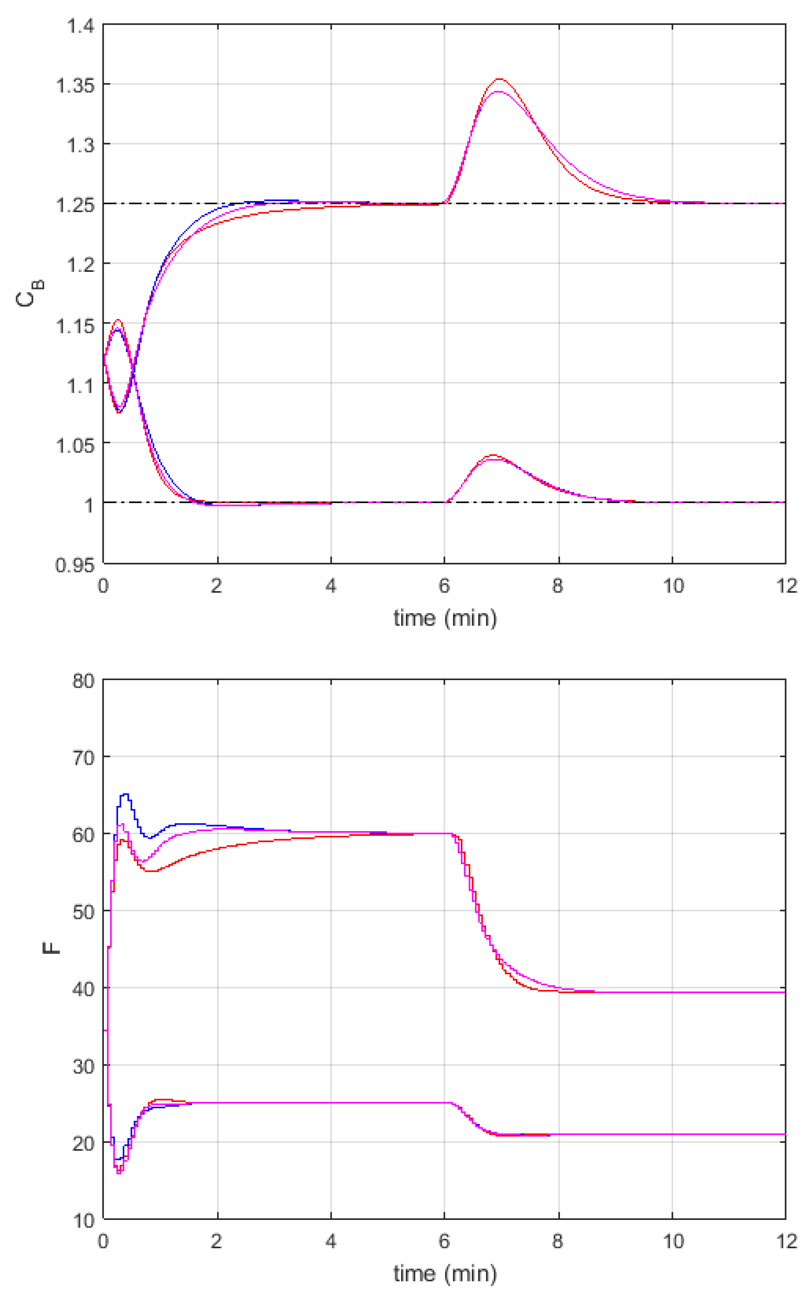
The FMPC2 and FMPC2a algorithms worked faster than FMPC1 and FMPC1a. However, the same relations between the algorithms could be observed when the responses generated with FMPC2 and FMPC2a algorithms were compared with the ones obtained with the NMPC algorithm (Figure 4). If the setpoint was changed to mol/L, the responses obtained with all the algorithms (FMPC2, FMPC2a, and NMPC) were very close to each other. There was almost no overshoot, and the FMPC2 algorithm was slightly slower than the other algorithms.
In the case when the setpoint changed to mol/L, the response obtained with the FMPC2 algorithm was the fastest one. The one generated with the NMPC algorithm was the slowest, and the response obtained with the FMPC2a algorithm, for the same reason as in the case of the FMPC1a algorithm, was between these two responses. In the case of all the algorithms, the setpoint was reached almost without overshoot.
The disturbance responses obtained with the FMPC2 and FMPC2a algorithms were practically the same (the same phenomenon was observed in the case of the FMPC1 and FMPC1a algorithms). Near mol/L and mol/L, the NMPC algorithm generated a bigger maximal error than the FMPC algorithms. In all three cases, there was no overshoot.
It can be noticed that the FMPC1a and FMPC2a algorithms generated responses closer to the ones generated by the NMPC algorithm than the FMPC1 and FMPC2 algorithms. This is because in the algorithms with the advanced construction of the dynamic matrix, the prediction was more accurate, thanks to using the proposed mechanism. It should be, however, emphasized that all the FMPC algorithms used a reliable quadratic programming routine to generate the control action instead of the non-convex, nonlinear optimization utilized in the NMPC algorithm. When comparing the SSE (Sum of Squared Errors), one can notice that the smallest value was obtained with the FMPC2 and FMPC2a algorithms. This is because they used the modified performance index in the optimization problem solved by the algorithm in each time step.
We also performed experiments with the changes of the parameters ( coefficient and the control horizon) of the algorithms, like the ones in [12]. First, the coefficient was changed to (Figure 5 and Figure 6). All the algorithms now worked faster than in the previous case (for ); the control action was more aggressive, and the maximal errors at the beginning of the experiment were now bigger. However, the relations between the FMPC and NMPC algorithms remained unchanged. It can be also noticed that the differences between the FMPC1a and FMPC2a (and also FMPC1 and FMPC2) algorithms became much smaller compared to the previous experiments. The FMPC1a algorithm was practically as fast as the FMPC2a one. This is because for , both performance indexes (42) and (47) were the same. Thus, the closer the value of the coefficient to zero is, the closer the responses generated with the FMPC1a and FMPC2a algorithms should be. The SSE values obtained for all the algorithms were smaller than in the previous case, i.e., for .
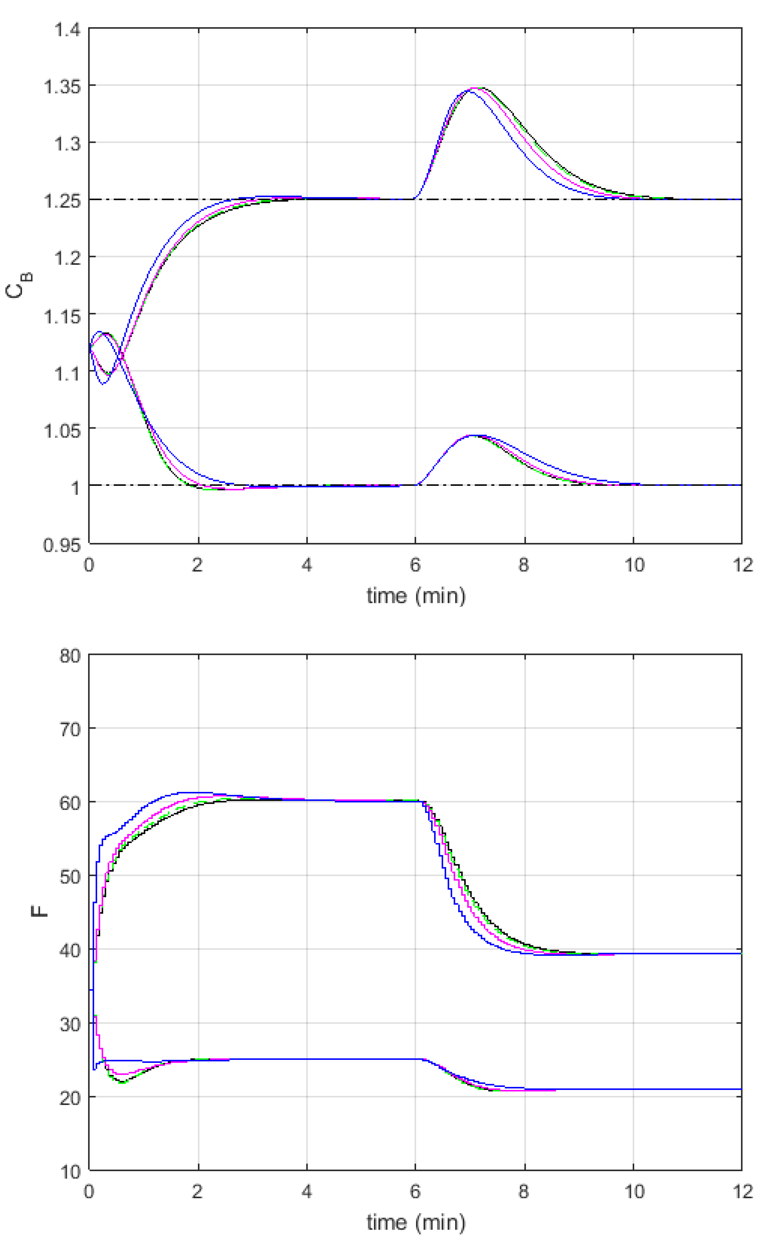
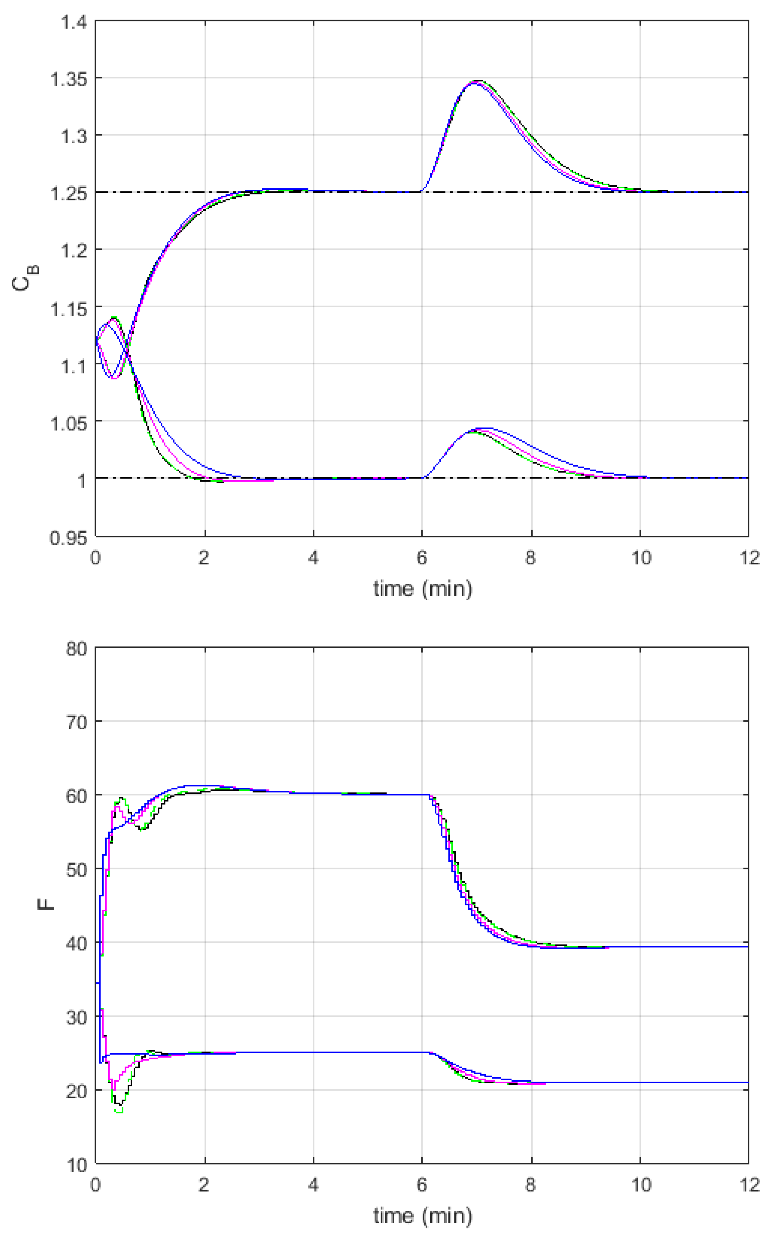
To simplify the optimization problem by reducing the number of decision variables, one can decrease the control horizon s. The responses obtained for different values of the control horizon are shown in Figure 7 and Figure 8 for the FMPC1a and FMPC2a algorithms, respectively. In the case of both algorithms, the control horizon can be shortened significantly, because the obtained responses do not change too much when the control horizon is between and . However, reduction of the control horizon should be done carefully, because for a too short control horizon, the control performance can get worse.
The FMPC1a algorithm, for , compensated the disturbance near mol/L faster, but achieved the setpoint mol/L slightly more slowly. A further decrease of the control horizon to brought faster disturbance compensation near mol/L, but worsened the compensation near mol/L. Reaching the setpoint mol/L was also faster, but at the cost of a slower response to the setpoint change to mol/L. The value of the SSE decreased with the decrease of the control horizon, but the value of the SSE obtained for was noticeably smaller than in the other cases.
The FMPC2a algorithm, for and , compensates the disturbance near mol/L slightly faster, but unfortunately reaching the setpoint mol/L took longer, especially for . Disturbance compensation near mol/L was also visibly slower for . The smallest value of the SSE was obtained for ; however, the differences in the SSE values in all cases were very small.
4. Conclusions
The mechanism for the advanced construction of the dynamic matrix proposed in the article uses the easy-to-obtain fuzzy model and advanced free response to generate the dynamic matrix skillfully. Thanks to such an approach, the changes of the operating point on the prediction horizon are taken into consideration during the construction of the dynamic matrix. This leads to obtaining a very good prediction, which is, however, linear with respect to the control changes. As a result, the FMPC algorithms can offer control performance very close to the one characteristic for the NMPC algorithms (based on the nonlinear optimization) and, at the same time, numerical efficiency resulting from the fact that the proposed mechanism is designed in such a way that the FMPC algorithms are formulated as the easy-to-solve quadratic optimization problems.
The proposed mechanism can be applied by a control system designer also in the case of simpler FMPC algorithms, e.g., with the classical free response. It should improve the operation of such a controller, but a better prediction can be obtained in the case considered in the article when the advanced free response is used. The quality of the advanced dynamic matrix and of the prediction can be increased even more if iterative improvement of the free response is applied.
Funding
This research received no external funding.
Conflicts of Interest
The author declares no conflict of interest.
Abbreviations
The following abbreviations are used in this manuscript:
| CSTR | Continuous Stirred-Tank Reactor |
| DMC | Dynamic Matrix Control |
| FMPC | Fuzzy Model Predictive Control |
| LMPC | Linear Model Predictive Control |
| LMIs | Linear Matrix Inequalities |
| MPC | Model Predictive Control |
| MIMO | Multiple-Input Multiple-Output |
| NMPC | Nonlinear Model Predictive Control |
| SSE | Sum of Squared Errors |
References
- Camacho, E.F.; Bordons, C. Model Predictive Control; Springer: London, UK, 1999. [Google Scholar]
- Domański, P.D. Performance Assessment of Predictive Control—A Survey. Algorithms 2020, 13, 97. [Google Scholar] [CrossRef] [Green Version]
- El Youssef, J.; Castle, J.; Ward, W.K. A Review of Closed—Loop Algorithms for Glycemic Control in the Treatment of Type 1 Diabetes. Algorithms 2009, 2, 518. [Google Scholar] [CrossRef] [Green Version]
- Maciejowski, J.M. Predictive Control with Constraints; Prentice Hall: Harlow, UK, 2002. [Google Scholar]
- Nebeluk, R.; Marusak, P. Efficient MPC algorithms with variable trajectories of parameters weighting predicted control errors. Arch. Control Sci. 2020, 30, 325–363. [Google Scholar]
- Plamowski, S.; Kephart, R.W. The Model Order Reduction Method as an Effective Way to Implement GPC Controller for Multidimensional Objects. Algorithms 2020, 13, 178. [Google Scholar] [CrossRef]
- Rossiter, J.A. Model–Based Predictive Control: A Practical Approach; CRC Press: Boca Raton, FL, USA, 2003. [Google Scholar]
- Sands, T. Comparison and Interpretation Methods for Predictive Control of Mechanics. Algorithms 2019, 12, 232. [Google Scholar] [CrossRef] [Green Version]
- Tatjewski, P. Advanced Control of Industrial Processes; Structures and Algorithms; Springer: London, UK, 2007. [Google Scholar]
- Blevins, T.L.; McMillan, G.K.; Wojsznis, W.K.; Brown, M.W. Advanced Control Unleashed; The ISA Society: Research Triangle Park, NC, USA, 2003. [Google Scholar]
- Ławryńczuk, M.; Marusak, P.; Tatjewski, P. Cooperation of model predictive control with steady–state economic optimisation. Control Cybern. 2008, 37, 133–158. [Google Scholar]
- Marusak, P. Numerically Efficient Fuzzy MPC Algorithm with Advanced Generation of Prediction: Application to a Chemical Reactor. Algorithms 2020, 13, 143. [Google Scholar] [CrossRef]
- Tatjewski, P. Disturbance modeling and state estimation for offset–free predictive control with state–spaced process models. Int. J. Appl. Math. Comput. Sci. 2014, 24, 313–323. [Google Scholar] [CrossRef] [Green Version]
- Abdelaal, M.; Schön, S. Predictive Path Following and Collision Avoidance of Autonomous Connected Vehicles. Algorithms 2020, 13, 52. [Google Scholar] [CrossRef] [Green Version]
- Chen, H.; Allgöwer, F. A Quasi-Infinite Horizon Nonlinear Model Predictive Control Scheme with Guaranteed Stability. Automatica 1998, 34, 1205–1217. [Google Scholar] [CrossRef]
- Tatjewski, P. Offset–free nonlinear model predictive control with state–space process models. Arch. Control Sci. 2017, 27, 595–615. [Google Scholar] [CrossRef] [Green Version]
- Diehl, M.; Bock, H.G.; Schlöder, J.P.; Findeisen, R.; Nagy, Z.; Allgöwer, F. Real–time optimization and nonlinear model predictive control of processes governed by differential–algebraic equations. J. Process Control 2002, 12, 577–585. [Google Scholar] [CrossRef]
- Schäfer, A.; Kühl, P.; Diehl, M.; Schlöder, J.; Bock, H.G. Fast reduced multiple shooting methods for nonlinear model predictive control. Chem. Eng. Process. 2007, 46, 1200–1214. [Google Scholar] [CrossRef]
- Zavala, V.M.; Laird, C.D.; Biegler, L.T. A fast moving horizon estimation algorithm based on nonlinear programming sensitivity. J. Process Control 2008, 18, 876–884. [Google Scholar] [CrossRef] [Green Version]
- Dominguez, L.F.; Pistikopoulos, E.N. A Novel mp-NLP Algorithm for Explicit/Multi-parametric NMPC. In Proceedings of the 8th IFAC Symposium on Nonlinear Control Systems, Bologna, Italy, 1–3 September 2010. [Google Scholar]
- Johansen, T.A. On multi–parametric nonlinear programming and explicit nonlinear model predictive control. In Proceedings of the 41st IEEE Conf Decision and Control, Las Vegas, NV, USA, 10–13 December 2002; Volume 3, pp. 2768–2773. [Google Scholar]
- Johansen, T.A. Approximate explicit receding horizon control of constrained nonlinear systems. Automatica 2004, 40, 293–300. [Google Scholar] [CrossRef] [Green Version]
- Pistikopoulos, E.N.; Dua, V.; Bozinis, N.A.; Bemporad, A.; Morari, M. On–line optimization via off–line parametric optimization tools. Comput. Chem. Eng. 2002, 26, 175–185. [Google Scholar] [CrossRef]
- Bemporad, A.; Morari, M.; Dua, V.; Pistikopoulos, E.N. The explicit linear quadratic regulator for constrained systems. Automatica 2002, 38, 3–20. [Google Scholar] [CrossRef]
- Bemporad, A.; Borrelli, F.; Morari, M. Piecewise linear optimal controllers for hybrid systems. In Proceedings of the 2000 American Control Conference, Chicago, IL, USA, 28–30 June 2000; Volume 2, pp. 1190–1194. [Google Scholar]
- Khooban, M.H.; Vafam, N.; Niknam, T. Optimal partitioning of a boiler–turbine unit for Fuzzy model predictive control. ISA Trans. 2016, 64, 231–240. [Google Scholar] [CrossRef]
- Kong, L.; Yuan, J. Disturbance–observer–based fuzzy model predictive control for nonlinear processes with disturbances and input constraints. ISA Trans. 2019, 90, 74–88. [Google Scholar] [CrossRef]
- Kong, L.; Yuan, J. Generalized Discrete–time Nonlinear Disturbance Observer Based Fuzzy Model Predictive Control for Boiler–Turbine Systems. ISA Trans. 2019, 90, 89–106. [Google Scholar] [CrossRef] [PubMed]
- Shen, D.; Lim, C.-C.; Shi, P. Robust fuzzy model predictive control for energy management systems in fuel cell vehicles. Control Eng. Pract. 2020, 98, 104364. [Google Scholar] [CrossRef]
- Wu, X.; Shen, J.; Li, Y.; Lee, K.Y. Fuzzy modeling and predictive control of superheater steam temperature for power plant. ISA Trans. 2015, 56, 241–251. [Google Scholar] [CrossRef] [PubMed]
- Marusak, P.; Tatjewski, P. Stability analysis of nonlinear control systems with unconstrained fuzzy predictive controllers. Arch. Control Sci. 2002, 12, 267–288. [Google Scholar]
- Killian, M.; Kozek, M. T–S fuzzy model predictive speed control of electrical vehicles. IFAC-Pap. Line 2017, 50, 2011–2016. [Google Scholar] [CrossRef]
- Marusak, P. Efficient model predictive control algorithm with fuzzy approximations of nonlinear models. LNCS 2009, 5495, 448–457. [Google Scholar]
- Ławryńczuk, M. Computationally Efficient Model Predictive Control Algorithms: A Neural Network Approach; Springer: Heidelberg, Germany, 2014. [Google Scholar]
- Morari, M.; Lee, J.H. Model predictive control: Past, present and future. Comput. Chem. Eng. 1999, 23, 667–682. [Google Scholar] [CrossRef]
- Boulkaibet, I.; Belarbi, K.; Bououden, S.; Marwala, T.; Chadli, M. A new T–S fuzzy model predictive control for nonlinear processes. Expert Syst. Appl. 2017, 88, 132–151. [Google Scholar] [CrossRef]
- Essien, E.; Ibrahim, H.; Mehrandezh, M.; Idem, R. Adaptive neuro-fuzzy inference system (ANFIS)—Based model predictive control (MPC) for carbon dioxide reforming of methane (CDRM) in a plug flow tubular reactor for hydrogen production. Therm. Sci. Eng. Prog. 2019, 9, 148–161. [Google Scholar] [CrossRef]
- Ławryńczuk, M. Nonlinear state–space predictive control with on–line linearisation and state estimation. Int. J. Appl. Math. Comput. Sci. 2015, 25, 833–847. [Google Scholar] [CrossRef] [Green Version]
- Marusak, P. Advantages of an easy to design fuzzy predictive algorithm in control systems of nonlinear chemical reactors. Appl. Soft Comput. 2009, 9, 1111–1125. [Google Scholar] [CrossRef]
- Lu, J.; Cao, Z.; Zhang, R.; Gao, F. Nonlinear Monotonically Convergent Iterative Learning Control for Batch Processes. IEEE Trans. Ind. Electron. 2018, 65, 5826–5836. [Google Scholar] [CrossRef]
- Lu, J.; Cao, Z.; Gao, F. 110th Anniversary: An Overview on Learning–Based Model Predictive Control for Batch Processes. Ind. Eng. Chem. Res. 2019, 58, 17164–17173. [Google Scholar] [CrossRef]
- Lu, J.; Cao, Z.; Zhao, C.; Gao, F. Multipoint Iterative Learning Model Predictive Control. IEEE Trans. Ind. Electron. 2019, 66, 6230–6240. [Google Scholar] [CrossRef]
- Marusak, P. Disturbance Measurement Utilization in the Efficient MPC Algorithm with Fuzzy Approximations of Nonlinear Models. LNCS 2013, 7824, 307–316. [Google Scholar]
- Takagi, T.; Sugeno, M. Fuzzy identification of systems and its application to modeling and control. IEEE Trans. Syst. Man Cybern. 1985, 15, 116–132. [Google Scholar] [CrossRef]
- Piegat, A. Fuzzy Modeling and Control; Physica–Verlag: Heidelberg, Germany, 2001. [Google Scholar]
- Marusak, P. Efficient fuzzy predictive algorithms with integrated economic optimization: A case study. IFAC Proc. Vol. 2007, 40, 61–66. [Google Scholar] [CrossRef]
- Marusak, P. Easily reconfigurable analytical fuzzy predictive controllers: Actuator faults handling. LNCS 2008, 5370, 396–405. [Google Scholar]
- Ribeiro, L.M.; Secchi, A.R. A methodology to obtain analytical models that reduce the computational complexity faced in real time implementation of NMPC controllers. Braz. J. Chem. Eng. 2019, 36, 1255–1277. [Google Scholar] [CrossRef] [Green Version]
- Mate, S.; Kodamana, H.; Bhartiya, S.; Nataraj, P.S.V. A Stabilizing Sub–Optimal Model Predictive Control for Quasi–Linear Parameter Varying Systems. IEEE Control Syst. Lett. 2020, 4, 402–407. [Google Scholar] [CrossRef]
- Jain, A.; Taparia, R. Laguerre function based model predictive control for van–de–vusse reactor. In Proceedings of the 2nd IEEE Int. Conf. Power Electronics, Intelligent Control and Energy Systems, ICPEICES 2018, Delhi, India, 22–24 October 2018; Volume 3, pp. 1010–1015. [Google Scholar]
- Uçak, K. A Runge–Kutta neural network-based control method for nonlinear MIMO systems. Soft Comput. 2019, 23, 7769–7803. [Google Scholar] [CrossRef]
- Uçak, K. A Novel Model Predictive Runge–Kutta Neural Network Controller for Nonlinear MIMO Systems. Neural Process. Lett. 2020, 51, 1789–1833. [Google Scholar] [CrossRef]
- Sang Nguyen, T.; Hoang, N.H.; Hussain, M.A. Tracking error plus damping injection control of non-minimum phase processes. IFAC-Pap. Line 2018, 51, 643–648. [Google Scholar] [CrossRef]
- Doyle, F.; Ogunnaike, B.A.; Pearson, R.K. Nonlinear model–based control using second–order Volterra models. Automatica 1995, 31, 697–714. [Google Scholar] [CrossRef]
Figure 1.
Steady-state characteristic of the control plant.

Figure 2.
Membership functions of the fuzzy model used to obtain the dynamic matrix.

Figure 3.
Responses of the control system to changes in the setpoint to mol/L and mol/L and to the change of the disturbance by 10% in the 6th minute of the experiment; ; NMPC—red lines (SSE = 1.2900), FMPC1—blue lines (SSE = 1.2764), FMPC1a—magenta lines (SSE = 1.2740).
Figure 3.
Responses of the control system to changes in the setpoint to mol/L and mol/L and to the change of the disturbance by 10% in the 6th minute of the experiment; ; NMPC—red lines (SSE = 1.2900), FMPC1—blue lines (SSE = 1.2764), FMPC1a—magenta lines (SSE = 1.2740).

Figure 4.
Responses of the control system to changes in the setpoint to mol/L and mol/L and to the change of the disturbance by 10% in the 6th minute of the experiment; ; NMPC—red lines (SSE = 1.2900), FMPC2—blue lines (SSE = 1.2230), FMPC2a—magenta lines (SSE = 1.2183).
Figure 4.
Responses of the control system to changes in the setpoint to mol/L and mol/L and to the change of the disturbance by 10% in the 6th minute of the experiment; ; NMPC—red lines (SSE = 1.2900), FMPC2—blue lines (SSE = 1.2230), FMPC2a—magenta lines (SSE = 1.2183).
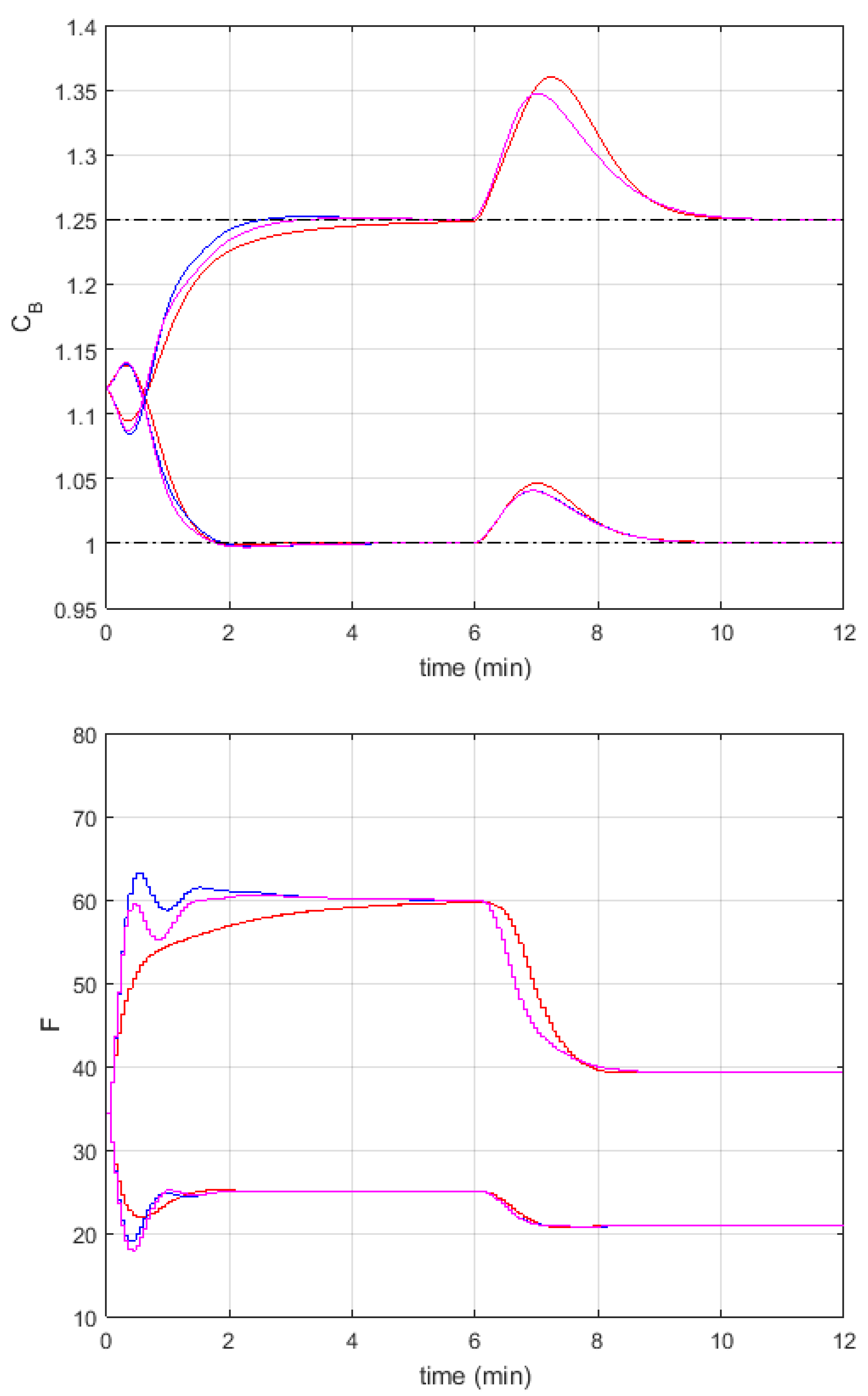
Figure 5.
Responses of the control system to changes in the setpoint to mol/L and mol/L and to the change of the disturbance by 10% in the 6th minute of the experiment; ; NMPC—red lines (SSE = 1.1913), FMPC1—blue lines (SSE = 1.1679), FMPC1a—magenta lines (SSE = 1.1629).
Figure 5.
Responses of the control system to changes in the setpoint to mol/L and mol/L and to the change of the disturbance by 10% in the 6th minute of the experiment; ; NMPC—red lines (SSE = 1.1913), FMPC1—blue lines (SSE = 1.1679), FMPC1a—magenta lines (SSE = 1.1629).

Figure 6.
Responses of the control system to changes in the setpoint to mol/L and mol/L and to the change of the disturbance by 10% in the 6th minute of the experiment; ; NMPC—red lines (SSE = 1.1913), FMPC2—blue lines (SSE = 1.1502), FMPC2a—magenta lines (SSE = 1.1450).
Figure 6.
Responses of the control system to changes in the setpoint to mol/L and mol/L and to the change of the disturbance by 10% in the 6th minute of the experiment; ; NMPC—red lines (SSE = 1.1913), FMPC2—blue lines (SSE = 1.1502), FMPC2a—magenta lines (SSE = 1.1450).

Figure 7.
Responses of the control system with FMPC1a algorithm and to changes in the setpoint to mol/L and mol/L and to the change of the disturbance by 10% in the 6th minute of the experiment; —black lines (SSE = 1.2740), —green dashed lines (SSE = 1.2675), —magenta lines (SSE = 1.2631), —blue lines (SSE = 1.2218).

Figure 8.
Responses of the control system with FMPC2a algorithm and to changes in the setpoint to mol/L and mol/L and to the change of the disturbance by 10% in the 6th minute of the experiment; —black lines (SSE = 1.2183), —green dashed lines (SSE = 1.2142), —magenta lines (SSE = 1.2220), —blue lines (SSE = 1.2218).

Publisher’s Note: MDPI stays neutral with regard to jurisdictional claims in published maps and institutional affiliations. |
© 2021 by the author. Licensee MDPI, Basel, Switzerland. This article is an open access article distributed under the terms and conditions of the Creative Commons Attribution (CC BY) license (http://creativecommons.org/licenses/by/4.0/).
Share and Cite
MDPI and ACS Style
Marusak, P.M. Advanced Construction of the Dynamic Matrix in Numerically Efficient Fuzzy MPC Algorithms. Algorithms 2021, 14, 25. https://0-doi-org.brum.beds.ac.uk/10.3390/a14010025
AMA Style
Marusak PM. Advanced Construction of the Dynamic Matrix in Numerically Efficient Fuzzy MPC Algorithms. Algorithms. 2021; 14(1):25. https://0-doi-org.brum.beds.ac.uk/10.3390/a14010025
Chicago/Turabian StyleMarusak, Piotr M. 2021. "Advanced Construction of the Dynamic Matrix in Numerically Efficient Fuzzy MPC Algorithms" Algorithms 14, no. 1: 25. https://0-doi-org.brum.beds.ac.uk/10.3390/a14010025
Note that from the first issue of 2016, this journal uses article numbers instead of page numbers. See further details here.