A Memetic Algorithm for an External Depot Production Routing Problem


1
Laboratoire de Recherche en Informatique et Télécommunication, Institut National Polytechnique Félix Houphouët-Boigny, Yamoussoukro, Cote d’Ivoire
2
Laboratoire des Sciences et Technologies de l’Information et de la Communication, École Supérieure Africaine des TIC, Abidjan, Cote d’Ivoire
*
Author to whom correspondence should be addressed.
Algorithms 2021, 14(1), 27; https://0-doi-org.brum.beds.ac.uk/10.3390/a14010027
Submission received: 25 November 2020
/
Revised: 9 January 2021
/
Accepted: 12 January 2021
/
Published: 19 January 2021
Abstract
:This study aims to compare the results of a memetic algorithm with those of the two-phase decomposition heuristic on the external depot production routing problem in a supply chain. We have modified the classical scheme of a genetic algorithm by replacing the mutation operator by three local search algorithms. The first local search consists in exchanging two customers visited the same day. The second consists in trying an exchange between two customers visited at consecutive periods and the third consists in removing a customer from his current tour for a better insertion in any tour of the same period. The tests that were carried out on 128 instances of the literature have highlighted the effectiveness of the memetic algorithm developed in this work compared to the two-phase decomposition heuristic. This is reflected by the fact that the results obtained by the memetic algorithm lead to a reduction in the overall average cost of production, inventory, and transport, ranging from 3.65% to 16.73% with an overall rate of 11.07% with regard to the results obtained with the two-phase decomposition heuristic. The outcomes will be beneficial to researchers and supply chain managers in the choice and development of heuristics and metaheuristics for the resolution of production routing problem.
1. Introduction
In the supply chain field, simultaneously planning production, inventories and distribution while minimizing the overall cost of these operations is a complex exercise known as the production routing problem (PRP) [1]. The PRP is a combination of two well-known problems in the literature. On the one hand, we have the lot sizing problem (LSP) and the vehicle routing problem (VRP) on the other hand. LSP determines the best trade-off between production and storage operations. The aim is to simultaneously determine the production schedule, quantities to be produced and quantities to be stored to minimize the overall cost of production and inventory. See [2] for more detailed literature review on the LSP.
VRP is a difficult NP-Hard problem as a particular case of the traveling salesman problem (TSP) which is itself a NP-Hard problem [3,4]. It consists of arranging routes between customers who must be visited at the same time based on the number of vehicles available and finding the best scheduling of visits to minimize the overall cost of transport over the planning horizon. Readers are also invited to see [5,6,7] for a review of the mathematical formulations of the problem and the methods or algorithms used to resolve it.
In the practice of industries, these two problems are disjointedly and sequentially analyzed. However, the work of Chandra et al. [8,9] have shown that it is possible to make gains of 3% to 20% on the overall cost of production and distribution by integrating and coordinating the decisions of LSP and VRP. This integrated and coordinated PRP is a NP-hard problem since it contains the VRP. In an integrated concept of supply chain planning, the customer no longer has exclusive control over decisions on his visit dates and quantities to be received. The implementation of new practices such as vendor managed inventory (VMI) and replenishment policies such as order-up-to-level (OU) and maximum level (ML) are necessary to achieve the goal of satisfying customer demand. VMI is a practice in which the supplier decides when and how much to deliver to the customer in a joint manner. He must also ensure that there is no shortage of stock at the customer. In the OU replenishment policy, all customers have maximum storage capacity and the amount delivered is such that the maximum level of storage is reached at each delivery. Whereas in the ML policy, all customers have maximum storage capacity and the quantity delivered is such that the maximum storage level is not exceeded at each delivery (). See [10,11,12,13] for more details on the practice of VMI and the use of OU and ML replenishment policies. A detailed literature review of PRP was provided by [1].
Although PRP is an NP-hard problem, exact methods for its resolution have been proposed. Among these exact approaches, the Lagrangian relaxation was one of the first methods proposed for the resolution of the PRP [14]. A branch-and-price algorithm was proposed to solve a PRP with the use of a homogeneous fleet of vehicles [15]. In a study using a single vehicle [16], the authors used a branch-and-cut (B&C) algorithm to solve the PRP problem. The B&C algorithm has also been proposed to solve the multivehicle version of the PRP [17].
Given the complexity of the PRP, several heuristics and metaheuristics have been developed for its resolution. In the first works on the PRP introduced by Chandra et al. [9], an H1 type decomposition method was proposed. The authors decomposed the problem into a capacitated LSP and VRP followed by some local search heuristics to solve the problem. Test results have shown that the integrated approach allows gains on the overall cost of operations ranging from 3% to 20%. Another two-phase decomposition method was presented for solving a PRP with a heterogeneous fleet of vehicles [18]. The authors used a mixed integer programming (MIP) to solve the first phase of the problem. This first phase of the problem concerns a problem of LSP with direct shipment (DS). In the second phase, an efficient algorithm was used to solve the VRP. It is a H2 type algorithm because the DS decisions are incorporated into the LSP, which is not the case for the H1 type algorithm. The H2 type of two-phase decomposition heuristic (TPDH) has also been used to solve a PRP with external depot (EDPRP) [19]. The authors used a MIP for solving the LSP problem with DS in the first phase and then used a genetic algorithm to solve the VRP in the second phase.
Metaheuristics are algorithms used to solve difficult combinatorial optimization problems. They are therefore master strategies that use other heuristics to find a better approximation of the best overall solution to an optimization problem. They are mostly used when a more efficient classical method to solve a given combinatorial optimization problem is not known. The high level of abstraction of metaheuristics makes them suitable for a wide range of problems. Thus, they find their application in various fields of scientific research.
Swarm intelligence (SI) is a family of metaheuristics that relies on nature through the interactions of agents (ants, bees, etc.) to solve complex optimization problems. SI has been used in wind energy potential analysis and wind speed forecasting to reduce the operating cost of wind farms [20]. The authors used a hybrid algorithm that combines the advantages of the genetic and adaptive particle swarm optimization (PSO) algorithm to optimize the weights and biases of the nonlinear network of extreme learning machines (ELMs) to efficiently improve the accuracy of the ELMs.
Another SI based on particle swarm optimization has been proposed for the analysis of handover in the field of spectrum sharing in mobile social networks [21]. With an increase in the globally adaptive inertia to 75.66% and an increase in data transfer rate of 47.29% compared to the IEEE802.16 protocol, the authors obtained a maximum mean signal-to-noise ratio of 14.8 dB. This value is the overall optimum that is required during handover for any mobile social network. Thus, the authors claim that their algorithm outperforms those in the mobile network literature by 75% by optimizing various aspects of handover.
In the age of big data, analyzing data and extracting relevant information from it is a challenge. A very important issue in this area is the selection of the most informative features in a dataset. Given the success of SI in solving difficult NP problems, it is increasingly used for selecting relevant characteristics in data analysis or in machine learning algorithms. A detailed literature review on the use of SI in feature selection is provided by [22]. The authors presented a unified SI Framework to explain the methods, techniques, and parameter choice in a SI algorithm for feature selection. They also presented the different datasets used to implement SI algorithms as well as the different SI algorithms.
Another literature review focusing on PSO algorithms and ACO algorithms as representative of SI was presented by [23]. The authors presented a description of the PSO and ACO algorithms as well as a state of the art on other SI algorithms. They also presented a status report on the use of SI in solving real life problems.
Regarding the use of SI in solving PRPs, a PSO algorithm has recently been proposed to solve the planning problem in an intelligent food logistics system model [24]. The authors have formulated the problem in a mixed integer multi-objective linear programming. Four objectives are addressed in this study. They are the minimization of total system expense, the maximization of average food quality, the minimization of the amount of CO2 emissions in transportation, and the production and minimization of total weighted delivery time. Tests conducted on small, medium, and large data sets resulted in cost reductions of 15.51% compared to a three-step decomposition method.
A self-adaptive evolutionary algorithm was proposed for berth planning in the operation of maritime container terminals [25]. The authors proposed a chromosome in which the probabilities of crossover and mutation are encoded in the chromosome. They focused their study on the comparison of several methods of parameter selection in evolutionary algorithms. On the one hand, there are the parameter tuning strategy approaches in which the values of the selected parameters remain unchanged throughout the execution of the algorithm. On the other hand, we have the parameter control approaches in which the parameters of the algorithm are adjusted throughout the execution of the algorithm according to certain strategies. Parameter control can be deterministic, adaptive, or self-adaptive. Test results show that the evolutionary algorithm of self-adaptive parameter control outperforms evolutionary algorithms using deterministic parameter control, adaptive parameter control and parameter tuning strategy by 4.01%, 6.83%, and 11.84% respectively based on the value of the objective function.
Another evolutionary algorithm was used to address a VRP in a “factory in box” [26]. This “factory in a box” concept involves assembling production modules into containers and transporting the containers to different customer sites. The authors modeled the problem as mixed integer programming to solve the problem and used CPLEX to solve the mathematical model of the problem. In addition to the evolutionary algorithm, they also proposed three metaheuristics including variable neighborhood search (VNS), taboo search (TS), and simulated annealing (SA) to solve the problem. The results of the tests carried out on large-sized instances show that the evolutionary algorithm provides better results than the other metaheuristics (VNS, TS, SA) developed to solve the problem.
Genetic algorithm (GA) is a stochastic strategy for solving complex optimization problems that takes better advantage of concepts from natural genetics and the theory of evolution. It is used to solve a production, inventory and distribution planning problem that takes into account several products. [27], the authors have solved the integrated problem of LSP and VRP. They also proposed integer programming to minimize the total cost of the system. Tests performed on small instances found an optimality deviation of 1.739% compared to the branch-and-bound (B&B) method. A multi-plant supply chain model with multiple customers was proposed by [28]. In this supply chain, products are delivered directly from the factory to the customers. The authors developed a hybrid AG to address the minimization of the overall cost of production and distribution. They used a multi-point crossover operator. This number of cut-off points is equal to the length of the chromosome divided by 4 with a 15% probability of crossover.
A greedy randomized adaptive search procedure (GRASP) has been proposed for solving a PRP involving a single type of product over a multi-period planning horizon with the use of a homogeneous fleet of vehicles [29]. The authors proposed three versions of GRASP for the integrated resolution of the PRP These are a classical GRASP, an improved version of GRASP with the incorporation of reactive mechanisms and a version of GRASP with a path reconnection process. Test results on 90 randomly generated instances with 50, 100 and 200 clients over 20 periods established the effectiveness of GRASP on the traditional method of breaking down the problem into sub-problems. These results also showed that GRASP with path re-connection and GRASP with reactive mechanisms give better results than traditional GRASP (without improvement). A GRASP has also been developed to solve a bi-objectives production and distribution problem [30]. These objectives concern the minimization of total production and distribution costs and the balancing of the total workload in the supply chain. They used a homogeneous fleet of vehicles to transport products. The results of tests on literature instances show that the GRASP developed allows a relatively small number of non-dominated solutions to be obtained in a very short computing time. Although the approximation of the Pareto front for each instance is discontinuous and not convex, it highlights the trade-off between the two objective functions.
A reactive tabu search was presented for solving a PRP to satisfy a time varying demand with a homogeneous fleet of vehicles over a finite planning horizon [31]. The authors compared the test results with the results obtained with GRASP on instances of up to 200 clients and 20 periods. This comparison revealed an improvement in results ranging from 10% to 20% on the overall cost of operations with an increase in computing time. A Tabu search (TS) with path relinking (TSPR) was used for PRP resolution with a homogeneous fleet of vehicles [32]. Tests performed on datasets from the literature have shown that TSPR gives better results than memetic algorithm with population management (MA|PM) and an improvement in results ranging from 2.20% to 8.78% compared to RTS.
An adaptive large neighborhood search (ALNS) procedure was used for computing the lower bound in the formulation of the multivehicle production and inventory routing problem (MVPRP) [33]. The results of tests carried out on small, medium, and large size instances established the effectiveness of ALNS on GRASP, MA|PM, RTS, and TSPR. The same authors also used ALNS for the computing of upper bounds in a B&C procedure for solving the MVPRP [17].
The variable neighborhood search (VNS) was developed for PRP resolution with a homogeneous fleet of vehicles [34]. The test results for this algorithm show that it is as competitive as the ALNS algorithm.
Introduced by Moscato [35], memetic algorithm (MA) is a powerful version of GA based on the use of local search to intensify the search in order to increase its efficiency. The preservation of diversity is crucial in evolutionary algorithms in general [36] and in GA in particular. Crossover and mutation operators are the best means of guaranteeing the diversity of the population from one generation to the next. A good strategy of combining diversification and intensification is the key to success which gives the MA a definite advantage over the GA.
In the area of chain supply planning, MA was used to resolve the LSP. In this problem family, MA has been proposed for a problem of stochastic multi-product sequencing and LSP [37]. It has also been used for LSP in soft drink plants [38] and for a multi-stage capacitated LSP [39]. For the VRP family, MA has been proposed for a VRP with time windows (VRPTW) [40,41]. See also [42,43] for the capacitated VRP as well as [44,45] for the use of heterogeneous fleets of vehicles. The use of MA is also very present in the optimization of integrated problems such as PRP. A MA with population management (MA|PM) has been developed by Boudia and Prins [46] to solve the integrated production, inventory, and distribution problem. The authors tackled a problem of simultaneous minimization of three costs consisting of the setup cost, the inventories cost and distribution cost. Tests on 90 randomly generated instances showed the efficiency of MA|MP compared to TPDH and GRAPS. The MA was also used in a study aimed at minimizing the overall cost of setup, inventory, and distribution in a multi-plant supply chain. In this supply chain, the information flow management system called “KANBAN” was implemented to manage information [47]. A real case study concerning the minimization of the overall cost of production and distribution was conducted in a large automotive company [48]. In this study, the authors modeled the problem as a non-linear mixed integer programming and used a custom MA for its resolution.
The MA used in this work is an adaptation of the one proposed by Boudia and Prins [46] to solve an integrated production, inventory, and distribution problem.
The remainder of this work is organized as follows: Section 2 is a description of the EDPRP. Section 3 shows the details of the MA used for EDPRP resolution. Section 4 highlights the conditions for experimentation and the comparison of the results obtained by the MA and the TPDH of H2 type. Finally, Section 5 provides a conclusion on the comparative study of MA and TPDH concerning EDPRP.
2. External Depot Production Routing Problem (EDPRP)
The EDPRP is an extension of the classic case of the PRP in which deterministic demands are met by a homogeneous fleet of vehicles over a discrete (multi-period) and finite planning horizon. In the EDPRP, the geographical position of a plant without storage capacity is different from that of the depot. The depot is supplied by the plant and the customer demand is only satisfied from the products stored at the depot. All vehicles start and end their trips at the depot. The collection of products from the plant to supply the depot is carried out either by vehicles that leave the depot and then collect a quantity of products directly from the plant and return to the depot, or by vehicles after satisfying the demand of one or more customers. In this extension of the PRP, products manufactured at the plant are not delivered directly to customers. The products are first stored at the depot before being delivered to customers. It is also important to note here that the quantities of products received by the depot in period are not distributed in the same period. These products must first be stored before distribution. Only the ML policy has been implemented in this work as a replenishment policy.
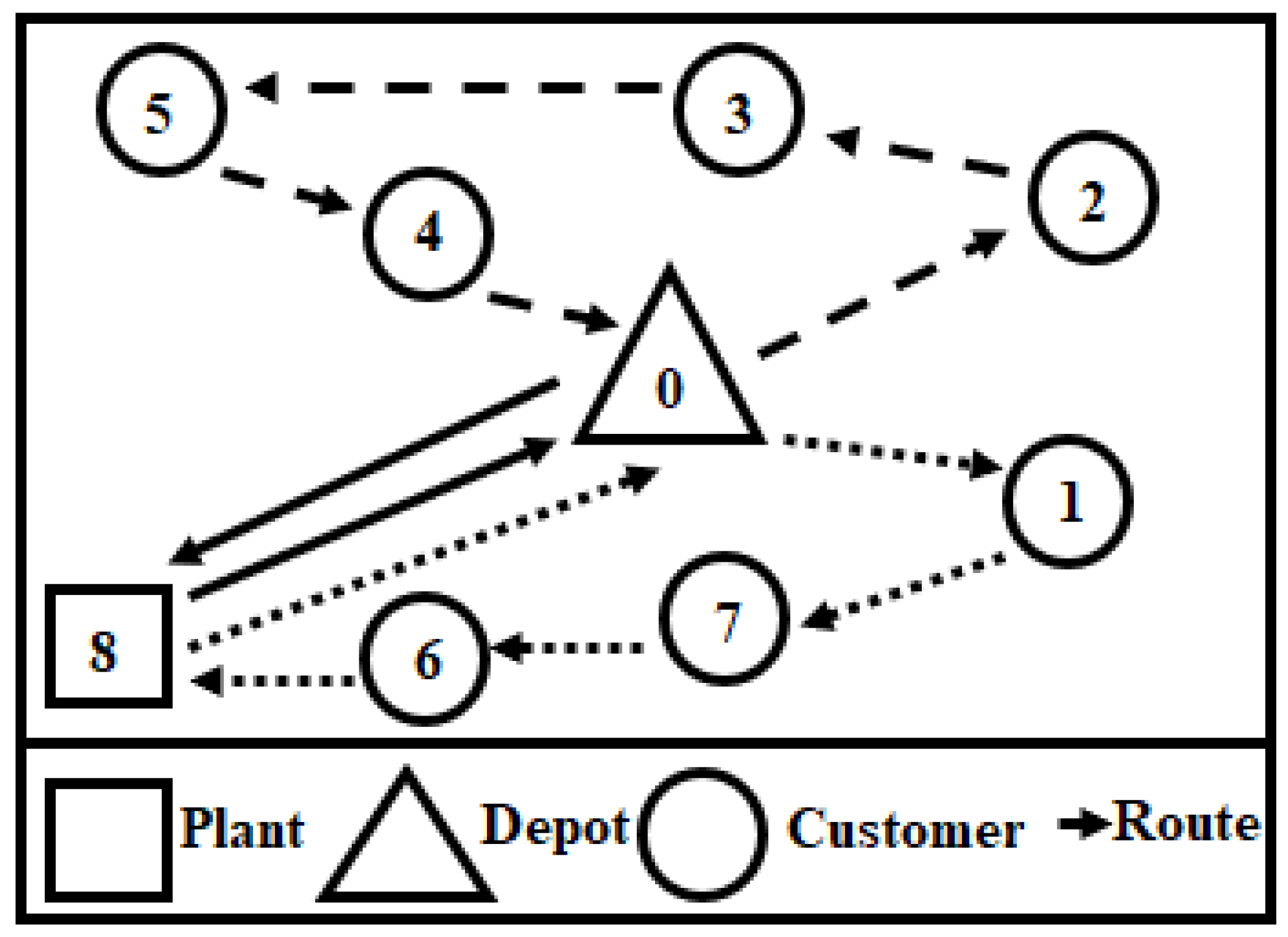
To describe the problem, the following elements have been defined: G = (N, A) is a complete graph in which N represents the set of nodes formed by the plant, the depot and the customers with the index i ∈ {0…n + 1} and A(N) = {(i, j): i, j ∈ N, i ≠ j} all the arcs in G. The plant is represented by n + 1, the depot is indexed by 0 and all customers are represented by is the set of customers. = {0, …, n} is the set made up by the depot and the customers. = {1, …, n + 1} is the set made up by the customers and the plant. N = {0, …, n + 1} is the set consisting of the depot, the customers, and the plant. T = {1, …, l} is the set of periods (days) of the planning horizon and K = {1, …, m} is the set of vehicles. See [19] for settings, variables and the MIP linking settings and variables. The product collection and distribution network in the EDPRP can be summarized in Figure 1. The authors. proposed a TPDH to solve the problem. In this work, we develop an MA to compare its results with those of the TPDH in the resolution of the EDPRP. The details of this MA are presented in the following section.
3. Memetic Algorithm
3.1. Encoding and Evaluating the Solution
3.1.1. Encoding
We use the tuple (P, Y, X, R) to describe a complete solution to the problem. In this tuple, P is a list of the quantity produced in each period t of the planning horizon. Each quantity produced or [t] is an integer between 0 and the maximum production capacity of the plant (C). Y is a list of binary numbers over each period t of the planning horizon. = 1 means that there is production at the plant on date t and 0 otherwise. X is a (n + 1) × matrix in which represents the amount of product sent to the depot (i = 0) or to a customer (. is an integer between 0 and the maximum storage capacity of the node and can be made up of several demands for the customer i. R is a list of integers with . It is a successive list of trips delimited by the symbol (0) when the trips belong to the same day or the symbol (−1) when the trips belong to different days. Thus 0 and −1 also refer to the depot in the modeling of the solution. As the symbol (−1) is also the day delimiter, a succession of this symbol indicates a period without a vehicle tour.
The knowledge of R, X and allows to compute for all and to verify the constraints related to the storage capacity of customers , the vehicle limit load (Q) as well as the limitation of the number of vehicles in the fleet (m). With the knowledge of Y, X, and , it is also possible to compute , and check the constraints on the storage capacity of the depot . The dataset of Table 1 allows to build an example of a complete solution for n = 10, l = 3, m = 2, C = 304 and Q = 198. This solution can be described by Table 2. In Table 2, R is a succession of trips that begin at the depot (0 or −1) and end at the depot over a planning horizon of 3 days (or three periods) delimited by the symbol −1. is the amount sent to each customer or depot i at the period t. The amount distributed to customers in the first period is 25 + 18 + 33 = 76. This quantity means that the demand of the first period is met based on the initial stocks of the depot ( = 76). No quantity is sent to the plant since it has no storage capacity. = 1 means that there is production in the first period of T. This automatically leads to a replenishment of the depot (0 or −1) with a quantity = 137 units of products. P and Y can therefore be represented by Y [0,0,1] and P [137,0,0]. Finally, with the knowledge of R, X, Y, and P it is possible to evaluate a solution.
3.1.2. Evaluation of the Solution
The cost (or fitness) of a solution Z can be determined by the following formula
In this three-part formula, denotes the total cost of production. This cost can be subdivided into two costs. Namely the variable cost of production defined by the sum of the costs of productions per period and the sum of setup costs when there is production on the day t (). Then we have the cost of the inventory expressed by and finally the cost of distribution (transport) represented by . In this last part, The |R| represents the size or number of symbols in R and alt( ) is a function such as alt(i) = i if and alt(i) = 0 if i = −1 (day delimiter). The parameter refers to the Euclidian distance between the i node and the node j.
3.2. Construction of the Initial Population
Let Pop_size be the size or number of individuals (solutions) in the initial population . This population consists of a Pop_size number of randomly generated solutions. Everyone in the initial population is generated in three steps described as follows:
- Step 1: Y construction.
The construction of Y consists in determining the days of production. Here, it is a question of determining the days t for which . To achieve this goal, we will first determine the total quantity produced over the planning horizon. Let NP be this quantity of products. It can be obtained by the following relationship: NP = . It is equal to the difference between the sum of the demands of all customers and the sum of the initial inventory at the depot and at the customers. Once the total quantity to be produced is calculated, we determine the number of days required to produce that quantity. To avoid a problem of hard bin packing with the limited fleet, we will limit the capacity of the fleet to 90%. Let be the capacity of the fleet and NY (NY = ) the number of days needed to produce NP. Then and NY are calculated as follows: and NY = . Once NY is determined, a NY number of days are randomly drawn in T/{}. It is not possible to produce on the last day of the planning horizon () because this production cannot be distributed to customers. Here, P can already be initialized by assigning NP to for which t is the smallest value of T having without considering the violation of maximum production capacity (C).
- Step 2: P and X construction day after day.
For any customer i, is initialized with the necessary quantity so that and at least constitute a demand (for each costumer i, ). For example, if the demand = 10, for = 5, we have on a = 5. For = 10, we have = 0 and for = 15 we have = 0. For each period t, giving priority to customers who are out of stock, we aggregate demands for each customer i without violating its storage limit capacity , and that of the fleet in respect of the quantity of products available at the depot the day before . The quantities produced are then adapted to the production capacity C and then to the capacity of the fleet and those of the depot . This makes it possible to resolve the production capacity overrun authorized in step 1. This approach is an adaptation of the dynamic programming (DP) proposed by Wagner and Whitin [49] for the resolution of the classic LSP.
- Step 3: Construction of R day after day.
After determining P and X, the quantities sent to customers per period are successively aggregated to reach the capacity of a vehicle This operation is repeated until the number of vehicles necessary to deliver the products of each period is determined. This procedure is an adaptation of Clarke and Wright’s economic algorithm [50] through the imposition of a limited fleet. At this stage, R does not yet contain the plant represented by the node i = n + 1. The plant is added to R only in the periods t for which = 1. The number of symbol n + 1 added is equal to the number of vehicles necessary to send all the production of the period t to the depot (for = 1 with t , the number of vehicles needed to transport from the plant to the depot is ). Once the initial population has been constituted, a selection and crossover procedure are carried out for the formation of the child population . In this study, the population size of children is set at POP_size/2. The following section describes the procedure of selection and crossover of parents of the initial population for the constitution of .
3.3. Selection and Crossover Procedure
Each child from the initial generation is the result of the crossover of two parents selected by a binary tournament procedure. A selection by binary tournament consists of selecting the best solution from two randomly drawn solutions in the population . Let A be the parent selected at the first selection procedure and B the parent selected at the second selection procedure. Then a two-point crossover procedure of parents A and B is implemented for the determination of a single child E. The crossover procedure can be described as follows: Let us note by () the membership operator. By this operator writing AR means that R belongs to A. Let us note or R(p) the element of rank p in R and or R(p→q) the sub-list of R going from p to q. In this work, the cutting points must correspond only to the day delimiter (−1). For the determination of cutting points, a random draw of two dates , with is made. Then and are determined so that and . Let pos(t) be the function that at each date associates its position in (p = pos(t)). will be segmented into three parts. The left part will be identified by . The middle of is represented by and the right part by . Similarly, parent B will also be segmented according to the values of and determined for the segmentation. The construction of child E from the crossover of A and B is done as follows: let , , and be the three parts of . These three parts will be initialized as follows: = , = and = . After the initialization of , a check is made to correct any anomalies in its construction. Contrary to Boudia et Prins’ correction strategy of browsing the symbols in [28] we adopt a simplified correction strategy of browsing the symbols in . This strategy allows to quickly identify the missing customers in and make the appropriate corrections. The correction is as follows: Let i be the browsing index of , the total quantity delivered to the customer i over T in and the total quantity of product that was to be delivered to i over T. We have = and . Through a comparison between and , We group customers into three subsets. The first subset is that of customers representing Case 1 such as = . The second subset representing Case 2 concerns the customers i for whom and Case 3 brings together the customers for whom . In the process of repairing the chromosome, all customers affected by Case 2 are treated first. Then come the customers concerned by Case 3 and finally those concerned by Case 1. Each case is treated as follows:
Case 1. If , then there is nothing to do for the costumer i. All demands are already met by the initial stock () and the quantities delivered over T ().
Case 2. If , then a reverse browsing of T is made (from i to 1). is successively reduced by a demand . For a given period t, if falls to 0 then i is removed from its trip at the date t in . This correction stops at the period t at which .
Case 3. If , let be the out-of-stock date at i if it is not supplied from the last date on which its initial stock covers its demands and the quantity needed to complete to . Browsing T from τ to , is corrected as follows:
- (1)
- If ≠ 0, then add to
- (2)
- If Q (vehicle limit capacity) is violated, then i is removed from its current tour.
- (3)
- Try the best insertion of i in one of the existing trips of the date t. Making the best insertion of a customer i in a trip is to compare the cost of all the trips obtained by iteratively moving the costumer i from the beginning of the tour to its end. The best insertion will designate the position of i offering the minimum transportation cost for the trip.
- (4)
- If the attempt at a better insertion fails and the number of vehicles used on the date t is less than m (m is the number of vehicles in the fleet) then a new trip is created.
- (5)
- If all the vehicles in the fleet are already in use, then we are fragmenting the quantity Fragmentation consists of determining the trip with the maximum residual capacity and inserting the maximum demand contained in . The rest of the quantities to be delivered ( after updating) are distributed at the following days. The correction stops when = 0.
NB: If τ = 1, then the quantity inserted is equal to the sum of the complement of the initial stock to a demand and a maximum number of demands .
However, if = 0, is corrected by implementing steps (3), (4), and (5).
3.4. Example of Application of the Crossover and Repair Procedure
Consider the dataset (n = 10, l = 6, k = 2) described in Table 3. Let A and B be two solutions got from the initial population. Chromosome A is represented by Table 4 and Solution B is represented by Table 5. Let = 3 and = 5 be the cut points of chromosomes A and B ( and correspond to dates or periods on the planning horizon). Child C represented in Table 6 will consist of three parties.
The left side of C is noted = ). The middle of C is and the right part of C is .
After the C chromosome is formed, abnormalities can be found. To repair the C chromosome, we go through the customers list and make the following corrections:
is the total amount of products that should have been received by customer i and the amount received by the customer i.
Customers for whom : i ∊ {3;4;8}
For the customer i = 3, we have = 60 + 15 = 75 and = 15 × 6 − = 90 − 30 = 60. By browsing T from t = 6 to t = 1, we subtract a demand to on the date t = 4 and we get = 75 − 15 = 60. Thus, the amount sent to i at period 4 becomes = 15 − 15 = 0 and i = 3 is removed from the tour of period 4. The result of this correction is shown in Table 7.
For the customer i = 4, we have = 49 and = 7 × 6 − 7 = 35. By browsing T from t = 6 to t = 1, we remove 2 demands in to the period t = 4 to get = 35 and = 21 − 7 − 7 = 7. See Table 8 for C chromosome after correction for i = 4.
For the customer i = 8, we have = 104 and = 13 × 6 − 13 = 65. The successive subtraction of a demand in to equalize allows to obtain the following results. Subtracting a demand from the period 6 allows to have = 104 − 13 = 91 and = 0. So, the customer 8 is removed from the tour of period 6. Subtracting two demands in in the period t = 4 allows to have = 91 − 13 − 13 = 65 and = 39 − 13 − 13 = 13. The result of this correction is presented in Table 9.
Customers for whom: : i ∊ {1;2;7}
For the customer i = 1, = 20 + 20 = 40 and = 6 × 10 − 10 = 50.
We have = 50 − 40 = 10. So, must be completed (management of a supplement) with a quantity of 10 products to reach . We have τ = and = + − 75 = 76 + 0 − 75 = 1; = + − 0 = 1 + 151 − 0 = 152; = + − 152 = 152 + 152 − 152 = 152. The quantity delivered to all customers in the period t = 4 is 20 + 7 + 13 + 44 = 84. So = + – 84 = 152 + 0 − 84 = 68 and > = 10. The tour of period 4 contains i = 1, so we apply (1) by adding to . We have = 10 + 20 = 30. This changes the vehicle’s load from 84 to 94 in period 4 for a maximum load of 198. The load of the vehicle is not violated, and the process stops for the customer i = 1. Table 10 illustrates the correction for customer i = 1.
For the customer i = 2, = 15 and = 60, hence = 60 − 15 = 45.
We have τ = and = + − 94 = 152 + 0 − 94 = 58 > . The tour of the period t = 4 does not contain i = 2, hence we apply the step (3) by making a better insertion of i = 2 in the tour of period t = 4. As a result of this insertion, the new load of the vehicle will be 139 < 198. The procedure stops for i = 2. The resulting chromosome is shown in Table 11.
For the customer i = 7, = 0 and = 22, hence = 22 − 0 = 22.
We have τ = and = + − 94 = 152 + 0 − 139 = 13; and = + − 0 = 13 + 44 = 57; = + − (16 + 19)= 57 + 0 − 35 = 22 ≥ . The tour of the period t = 6 does not contain i = 7, hence we apply the stage (3) by also making a better insertion of i = 7 in the tour of the period 6. As a result of this insertion, the new load of the vehicle will be 16 + 19 + 22 = 57 < 198. The procedure stops for i = 2. It is noticeable here that = 0 after the delivery of the customer 7 (see Table 12).
Customers for whom = : i ∊ {5;6;8;9;10}.
For customers 5, 6, 8, 9, and 10 there is nothing to do because the theoretical amount to be received is equal to the amount received. The result of this repair procedure is presented in Table 13.
3.5. Local Search Procedures
Three local search algorithms have been developed for the intensification phases of MA. , these algorithms can be described as follows:
SWAP1 (S1): It is a local search algorithm which allows to exchange the position of two customers i and j during the same period t (∀t ∈ T) in accordance with the capabilities of the vehicles assigned to transport the products. This exchange is only possible if customer i and j are visited on the same date t regardless they belong to the same trip.
BEST INSERTION (BI): The BI consists in removing customer i from its current trip on the date t and searching in all existing trips on the date t the position that offers the minimum cost of transport in accordance with the capacity of the vehicles .
SWAP2 (S2): This algorithm consists of exchanging two customers i and j visited respectively at consecutive periods t and t + 1. If that does not cause a stock outage and meets the conditions of maximum capacity of production C, storage (), and vehicles Q, the resulting solution is compared to the best current solution .
3.6. Global Description of the MA
Let be the population of the generation g with ( is the initial population). the maximum number of generations, the population of children and the end criterion. The MA used in this work can be described by the algorithm in Algorithm 1.
| Algorithm 1. Memetic Algorithm |
 |
4. Experimentations and Results
4.1. Experimentation
The MA described in Figure 2 is implemented in C++ on a 64-bit Intel Pentium Dual Core 1.60 GHz personal computer with 4 GB RAM. Details of the instances used in the various simulations can be found in [19].
In this work, the mutation operator is replaced by a local search and the selection of parents is done by a binary tournament procedure. Thus, the relevant parameters of the MA developed are the size of the population (Pop_Size), the maximum number of generations (max_gen) and the probability with which the local search (LS_search_prob) is applied to each solution. A strategy of adjustment of the parameters based on experimental comparisons (testing combinations of three values designating the size of the population, three values each representing the maximum number of generation and three rates designating the probability of local searches) was carried out on the four classes of instances with 20 clients, six periods, and two vehicles. A total of 3 × 3 × 3 × 4 = 108 tests allowed to retain the best parameters presented in the Table 14. This parameter tuning strategy is opposed to other methods based on parameter control. For a better understanding of parameter handling, see [25].
The aim of this study is to compare the results of the MA with those obtained with the two-phase decomposition heuristic (TPDH). To achieve this goal, several tests are conducted to evaluate the effectiveness of each local search algorithm as well as the combination of some of them.
4.2. Results
The tests performed on 128 instances have yielded the averages over the four classes of instances represented by the rows in Table 15.
In this table, %Diff denote the percentage difference between the cost determined with the MA and the cost determined with the TPDH. This rate of change determines the relative evolution of the results of the MA compared to the TPDH. The column Instance with the sub-columns n, l, m designates the instances used for tests with n clients, l periods on the planning horizon and m vehicles. The columns SWAP1, BI, SWAP2, BI&SWAP2, SWAP1& SWAP2, and ALL contain the sub-columns of the total cost percentage difference and the CPU percentage difference of the corresponding local search algorithms.
In Table 15, the combination of local search SWAP1 and SWAP2 (SWAP1&SWAP2) offers the best percentage difference with an overall average decrease of 10.50% in the cost obtained with MA compared to TPDH. The second-best combination of local search algorithms is the use of BI and SWAP2 (BI &SWAP2) with an overall reduction of 10.23% on the total cost of production, storage, and vehicle rounds. In this experiment, it was found that the combination of all local searches is less efficient than the combination of two of them. In terms of calculation time, only the use of BI as a local search method offers a reduction in calculation time of 36.85% (%Diff CPU = −36.85% in the Table 15). Although it has produced the largest number of better solutions, MA with a combination of SWAP1 and SWAP2 local searches shows an overall relative increase of 1759.09% in computation time compared to TPDH. Out of 192 (32 × 6) results obtained on all tests, TPDH obtained better results on only three tests concerning instances (n = 40, l = 3, m = 3) with the use of the local search methods BI, SWAP2 and the combination of SWAP1 and SWAP2 which gives a very low rate of 1.56% (3/192). The best solution for each of the 32 instances is obtained with the MA. Table 16 shows the distribution of the best solutions according to the local search method or combination of local search methods used, considering both the overall cost and the computation time.
In Table 16, Nbr_BS refers to the number of best solutions obtained with each local search method in the implementation of MA. According to Table 15 and Table 16, the local search methods BI, SWAP1(S1) and SWAP2(S2) individually had the same number of best solutions in the implementation of MA. Thus, each local search taken individually yielded 2 best results out of the 32 average results, i.e., a rate of 6.25% each. The combination of all the local search methods (ALL) also resulted in two best results, which also corresponds to a rate of 6.25% (100 × (2/32)). The highest number of best solutions was obtained with the combination of the local search methods SWAP1 and SWAP2. This combination alone represents the 17 best results out of the 32 in Table 16, a rate of 53.125%. The second-best combination is the one using BI and SWAP2. This combination yielded 7 best solutions out of 32 with a rate of 21.875%. In Table 17, each row gives details of the best solution for each instance in Table 15. The columns PROD, INV, and TRANS indicate the average production, storage, and transport costs (vehicle trips) of the best solution obtained with MA, respectively. COST is the average total cost of production, storage, and distribution (transport). RL refers to the local search used to obtain this result. Overall, Table 17 shows that the share of production cost in the overall cost is 72.87% (100 × (72,758.91/99,847.04)). The overall cost of storage accounts for 11.39% (100 × (11,372.73/99,847.04)) of the overall cost and the cost of vehicle rounds (distribution) accounts for 15.74% (100 × (15,715.41/99,847.04)) of the overall cost.
Table 18, Table 19 and Table 20 provide details of the comparison of production, storage, and distribution costs, respectively. In Table 18, all production costs obtained with the MA are less than or equal to the production costs of the TPDH.
The costs of production for 16 cases resolved with MA are invariant to the costs of production for TPDH, which corresponds to 50% of the relative results in Table 18. Overall, there is an average decrease of 5.18% in the cost of production obtained with the MA method compared to TPDH.
Regarding inventory (storage) cost, there is an increase in the average inventory costs on all instances with an overall average of 9887.34 for the cost obtained with the TPDH method against and a cost of 11,372.73 for the MA. The overall average increase in inventory costs from tests with MA is 15.38% relative to the cost obtained with the TPDH method.
Contrary to the inventory costs, a decrease in distribution cost is observed on all results obtained with the MA compared to the costs calculated with the TPDH. We have an overall average of 24,147.83 of the costs with TPDH against an overall average of 15,715.41 of the costs obtained with the MA. The overall average of percentage difference in the distribution cost calculated with the MA compared to the distribution cost calculated with the TPDH is −35.60%. This reflects an overall average decrease of 35% in the distribution cost obtained with the MA compared to the TPDH. Table 21 shows a comparison of the total cost constituted by the production, inventory and distribution cost obtained with the MA compared to the cost calculated with the TPDH. With an average overall cost of 112,783.76 for TPDH compared to 99,847.04 for MA, there is a decrease ranging from 3.65% to 16.73% on all total costs calculated with MA compared to TPDH with an average overall decrease of 11.07%. With an overall average computation time of 459.51 for TPDH compared to 280.98 for MA, there is an overall average increase of 1485.59% in the computation time for MA compared to TPDH. This is since the average does not consider the relative dispersion of computation times.
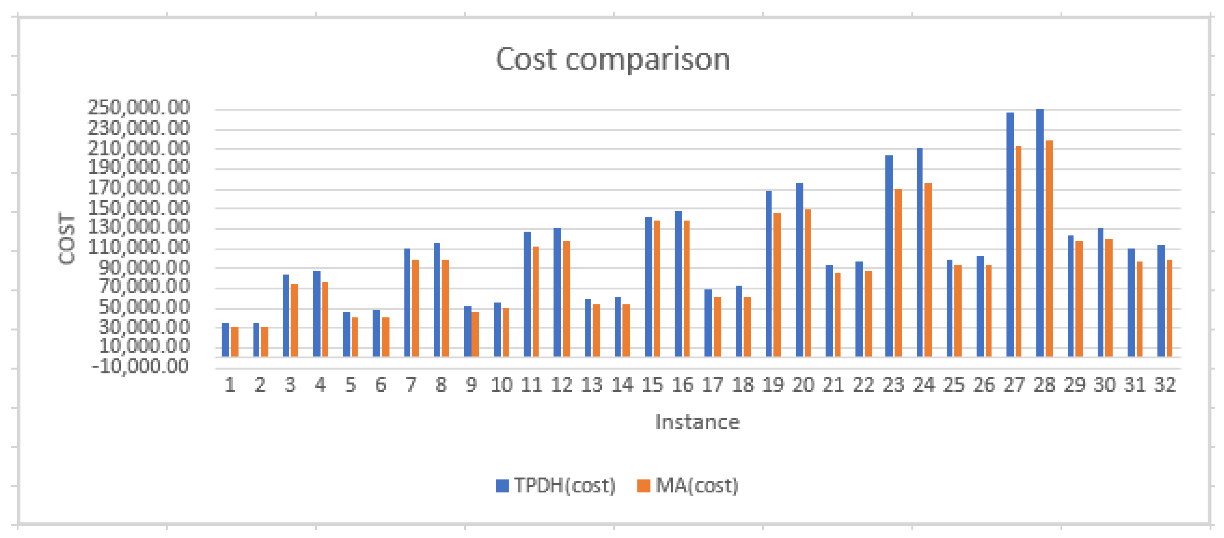
Figure 2 highlights the effectiveness of MA in reducing the overall cost of production, inventory, and distribution compared to TPDH. In this figure, we can see that the use of MA reduces the overall cost of operations. This reduction varies between 3614 and 35,339.
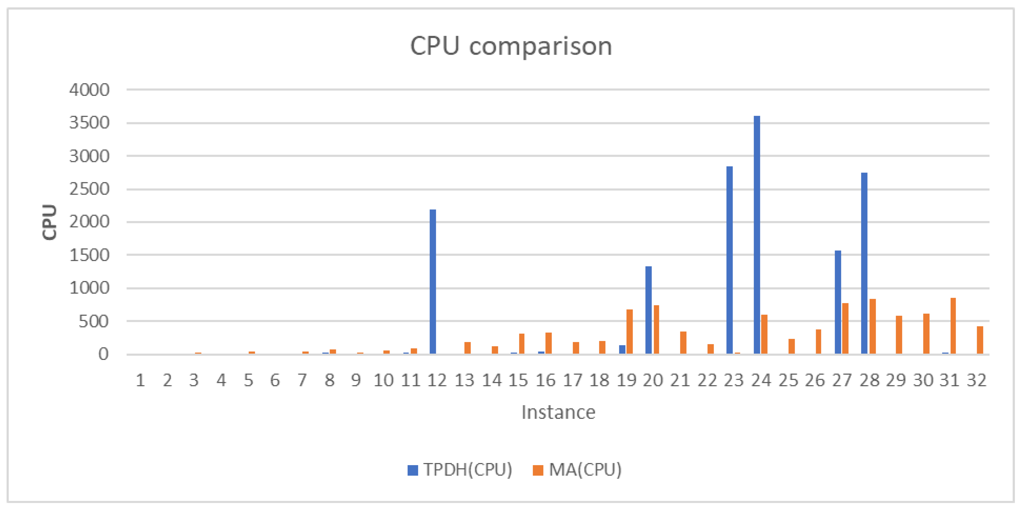
Figure 3 shows an increase in the calculation time with MA on all instances except instances 12, 20, 23, 24, and 28. For these instances, 95% of the computation time is consumed by the first phase with the use of CPLEX to solve an LSP problem with direct delivery.
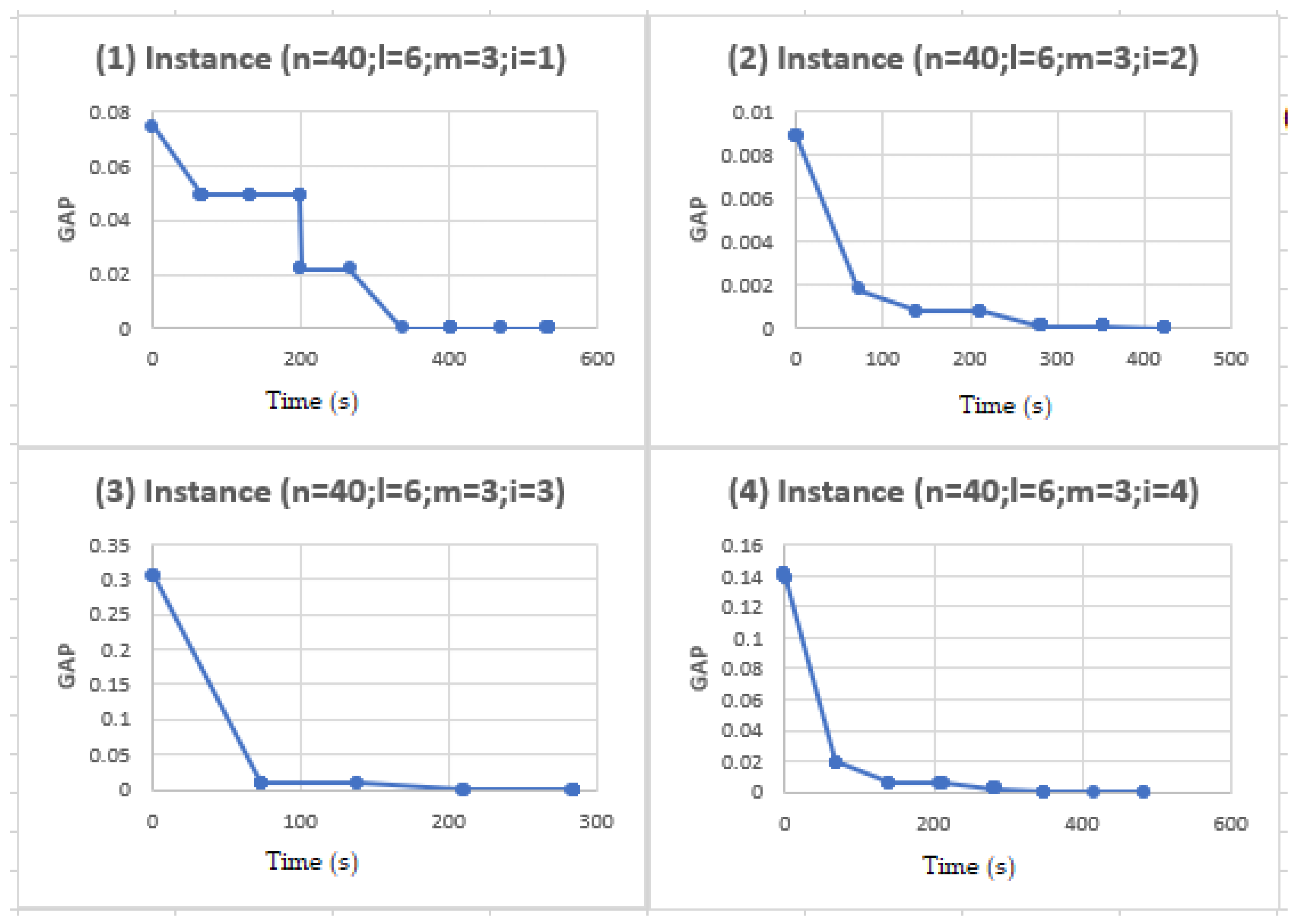
Figure 4 shows a general evolution of the MA algorithm for EDPRP like the one presented by [34,51]. In this figure, instances (1), (2), (3), and (4) are representative of the four classes of instances used to conduct tests on the dataset. These instances consisting of 40 clients (n = 40), six periods (l = 6), and three vehicles highlight the general behavior of the MA. The figure shows that the memetic algorithm proposed for the EDPRP converges rapidly from relatively bad solutions to good solutions.
5. Conclusions
This paper focuses on the comparative study of the results obtained with a memetic algorithm (MA) and a two-phase decomposition heuristic (TPDH) for the management of an external depot in a production routing problem (EDPRP). In the MA developed in this work, three local search algorithms (LS) were used to intensify the search for the best solution on each instance adapted from the work of Adulyasak and al. [17]. The results have shown an improvement in the production cost computed with MA compared to TPDH ranging from 0% to 16.64% with an overall average rate of 5.18%. Similarly, there has been an improvement in the cost of transport ranging from 17.08% to 51.26% with an overall average rate of 35.60%. However, the inventory cost increased from 5.69% to 32.10% with an overall average increase rate of 15.38%. As regards the overall cost of production, inventory and distribution, there was a reduction ranging from 3.65 to 16.73% with an overall rate of 11.07%. Such a finding highlights the effectiveness of MA in relation to TPDH.
Beyond the contributions developed in this work, many avenues of research remain to be examined. MA using the local search method BI is the only one that provides a reduction (36.85%) in MA computation time compared to TPDH with an overall average time of 12.87 s. This implementation of the MA allowed to obtain two better results with a decrease of 8.94% of the total global average cost compared to the TPDH. The use of MA with local search BI thus appears as a very good algorithm in the search for a good initial solution in the global scheme of a branch-and-cut algorithm.
In the model studied in this paper, the supply chain consists of a factory and a depot. Studies of versions with several factories and/or depots will help to reflect certain realities in supply chain practice and management. Similarly, considering certain characteristics such as the use of heterogeneous vehicles, dynamic (stochastic) demands or delivery from the plant during production days would also make it possible to highlight other aspects of realities in supply chain management.
A comparative study on the management of MA parameters could reveal other potentials of this algorithm. For example, this study would allow to compare the strategy of parameter tuning by the three methods of parameter control which are: deterministic parameter control, adaptive parameter control, and self-adaptive parameter control.
Author Contributions
Conceptualization, B.K.B.K. and M.D.; Data curation, B.K.B.K. and M.K.; Formal analysis, B.K.B.K., M.D. and M.K.; Investigation, B.K.B.K., M.D. and M.K.; Methodology, B.K.B.K.; Project administration, B.K.B.K. and S.O.; Resources, B.K.B.K., M.D. and M.K.; Software, B.K.B.K. and M.D.; Supervision, B.K.B.K. and S.O.; Validation, B.K.B.K., M.D., M.K. and S.O.; Visualization, B.K.B.K., M.D. and M.K.; Writing—original draft, B.K.B.K.; Writing—review and editing, M.D., M.K., and S.O. All authors have read and agreed to the published version of the manuscript.
Funding
This research received no external funding.
Conflicts of Interest
The authors declare no conflict of interest.
References
- Adulyasak, Y.; Cordeau, J.-F.; Jans, R. The production routing problem: A review of formulations and solution algorithms. Comput. Oper. Res. 2015, 55, 141–152. [Google Scholar] [CrossRef]
- Pochet, Y.; Wolsey, L.A. Production Planning by Mixed Integer Programming; Springer: New York, NY, USA; Berlin, Germany, 2006. [Google Scholar]
- Garey, M.R.; Johnson, D.S. Computers and Intractability; A Guide to the Theory of NP-Completeness; W.H. Freeman & Co.: New York, NY, USA, 1990; ISBN 978-0-7167-1045-5. [Google Scholar]
- Lenstra, J.K.; Kan, A.H.G. Complexity of vehicle routing and scheduling problems. Networks 1981, 11, 221–227. [Google Scholar] [CrossRef] [Green Version]
- Braekers, K.; Ramaekers, K.; Van Nieuwenhuyse, I. The vehicle routing problem: State of the art classification and review. Comput. Ind. Eng. 2016, 99, 300–313. [Google Scholar] [CrossRef]
- Eksioglu, B.; Vural, A.V.; Reisman, A. The vehicle routing problem: A taxonomic review. Comput. Ind. Eng. 2009, 57, 1472–1483. [Google Scholar] [CrossRef]
- Montoya-Torres, J.R.; López Franco, J.; Nieto Isaza, S.; Felizzola Jiménez, H.; Herazo-Padilla, N. A literature review on the vehicle routing problem with multiple depots. Comput. Ind. Eng. 2015, 79, 115–129. [Google Scholar] [CrossRef]
- Chandra, P. A dynamic distribution model with warehouse and customer replenishment requirements. J. Oper. Res. Soc. 1993, 44, 681–692. [Google Scholar] [CrossRef]
- Chandra, P.; Fisher, M.L. Coordination of production and distribution planning. Eur. J. Oper. Res. 1994, 72, 503–517. [Google Scholar] [CrossRef]
- Archetti, C.; Boland, N.; Grazia Speranza, M. A Matheuristic for the Multivehicle Inventory Routing Problem. Inf. J. Comput. 2017, 29, 377–387. [Google Scholar] [CrossRef]
- Archetti, C.; Speranza, M.G. The inventory routing problem: The value of integration: The inventory routing problem: The value of integration. Int. Trans. Oper. Res. 2016, 23, 393–407. [Google Scholar] [CrossRef]
- Bertazzi, L.; Speranza, M.G. Inventory routing problems: An introduction. EURO J. Transp. Logist. 2012, 1, 307–326. [Google Scholar] [CrossRef] [Green Version]
- Coelho, L.C.; Cordeau, J.-F.; Laporte, G. Thirty Years of Inventory Routing. Transp. Sci. 2014, 48, 1–19. [Google Scholar] [CrossRef]
- Fumero, F.; Vercellis, C. Synchronized Development of Production, Inventory, and Distribution Schedules. Transp. Sci. 1999, 33, 330–340. [Google Scholar] [CrossRef]
- Bard, J.F.; Nananukul, N. A branch-and-price algorithm for an integrated production and inventory routing problem. Comput. Oper. Res. 2010, 37, 2202–2217. [Google Scholar] [CrossRef]
- Archetti, C.; Bertazzi, L.; Paletta, G.; Speranza, M.G. Analysis of the maximum level policy in a production-distribution system. Comput. Oper. Res. 2011, 38, 1731–1746. [Google Scholar] [CrossRef]
- Adulyasak, Y.; Cordeau, J.-F.; Jans, R. Formulations and Branch-and-Cut Algorithms for Multivehicle Production and Inventory Routing Problems. Inf. J. Comput. 2014, 26, 103–120. [Google Scholar] [CrossRef]
- Lei, L.; Liu, S.; Ruszczynski, A.; Park, S. On the integrated production, inventory, and distribution routing problem. IIE Trans. 2006, 38, 955–970. [Google Scholar] [CrossRef] [Green Version]
- Kayé, B.K.B.; Diaby, M.; N’Takpé, T.; Oumtanaga, S. Managing an External Depot in a Production Routing Problem. IJACSA 2020, 11, 321–330. [Google Scholar] [CrossRef]
- Zhao, X.; Wang, C.; Su, J.; Wang, J. Research and application based on the swarm intelligence algorithm and artificial intelligence for wind farm decision system. Renew. Energy 2019, 134, 681–697. [Google Scholar] [CrossRef]
- Anandakumar, H.; Umamaheswari, K. A bio-inspired swarm intelligence technique for social aware cognitive radio handovers. Comput. Electr. Eng. 2018, 71, 925–937. [Google Scholar] [CrossRef]
- Brezočnik, L.; Fister, I.; Podgorelec, V. Swarm Intelligence Algorithms for Feature Selection: A Review. Appl. Sci. 2018, 8, 1521. [Google Scholar] [CrossRef] [Green Version]
- Slowik, A.; Kwasnicka, H. Nature Inspired Methods and Their Industry Applications—Swarm Intelligence Algorithms. IEEE Trans. Ind. Inf. 2018, 14, 1004–1015. [Google Scholar] [CrossRef]
- Chan, F.T.S.; Wang, Z.X.; Goswami, A.; Singhania, A.; Tiwari, M.K. Multi-objective particle swarm optimisation based integrated production inventory routing planning for efficient perishable food logistics operations. Int. J. Prod. Res. 2020, 58, 5155–5174. [Google Scholar] [CrossRef]
- Dulebenets, M.A.; Kavoosi, M.; Abioye, O.; Pasha, J. A Self-Adaptive Evolutionary Algorithm for the Berth Scheduling Problem: Towards Efficient Parameter Control. Algorithms 2018, 11, 100. [Google Scholar] [CrossRef] [Green Version]
- Pasha, J.; Dulebenets, M.A.; Kavoosi, M.; Abioye, O.F.; Wang, H.; Guo, W. An Optimization Model and Solution Algorithms for the Vehicle Routing Problem With a “Factory-in-a-Box”. IEEE Access 2020, 8, 134743–134763. [Google Scholar] [CrossRef]
- Mak, K.L. Design of integrated production-inventory-distribution systems using genetic algorithm. In Proceedings of the 1st International Conference on Genetic Algorithms in Engineering Systems: Innovations and Applications (GALESIA), Sheffield, UK, 12–14 September 1995; pp. 454–460. [Google Scholar]
- Chan, F.; Chung, S.; Wadhwa, S. A hybrid genetic algorithm for production and distribution. Omega 2005, 33, 345–355. [Google Scholar] [CrossRef]
- Boudia, M.; Louly, M.A.O.; Prins, C. A reactive GRASP and path relinking for a combined production–distribution problem. Comput. Oper. Res. 2007, 34, 3402–3419. [Google Scholar] [CrossRef]
- Casas-Ramírez, M.-S.; Camacho-Vallejo, J.-F.; González-Ramírez, R.G.; Marmolejo-Saucedo, J.-A.; Velarde-Cantú, J.-M. Optimizing a Biobjective Production-Distribution Planning Problem Using a GRASP. Available online: https://www.hindawi.com/journals/complexity/2018/3418580/abs/ (accessed on 12 January 2021).
- Bard, J.F.; Nananukul, N. The integrated production–inventory–distribution–routing problem. J Sched. 2009, 12, 257. [Google Scholar] [CrossRef]
- Armentano, V.A.; Shiguemoto, A.L.; Løkketangen, A. Tabu search with path relinking for an integrated production–distribution problem. Comput. Oper. Res. 2011, 38, 1199–1209. [Google Scholar] [CrossRef] [Green Version]
- Adulyasak, Y.; Cordeau, J.-F.; Jans, R. Optimization-Based Adaptive Large Neighborhood Search for the Production Routing Problem. Transp. Sci. 2014, 48, 20–45. [Google Scholar] [CrossRef]
- Qiu, Y.; Wang, L.; Xu, X.; Fang, X.; Pardalos, P.M. A variable neighborhood search heuristic algorithm for production routing problems. Appl. Soft Comput. 2018, 66, 311–318. [Google Scholar] [CrossRef]
- Moscato, P.; Cotta, C. A gentle introduction to memetic algorithms. In Handbook of Metaheuristics; Springer: New York, NY, USA; Berlin, Germany, 2003; pp. 105–144. [Google Scholar]
- Hertz, A.; Widmer, M. Guidelines for the use of meta-heuristics in combinatorial optimization. Eur. J. Oper. Res. 2003, 151, 247–252. [Google Scholar] [CrossRef]
- Schemeleva, K.; Delorme, X.; Dolgui, A.; Grimaud, F. Multi-product sequencing and lot-sizing under uncertainties: A memetic algorithm. Eng. Appl. Artif. Intell. 2012, 25, 1598–1610. [Google Scholar] [CrossRef]
- Toledo, C.F.; Arantes, M.S.; França, P.M.; Morabito, R. A memetic framework for solving the lot sizing and scheduling problem in soft drink plants. In Variants of Evolutionary Algorithms for Real-World Applications; Springer: New York, NY, USA; Berlin, Germany, 2012; pp. 59–93. [Google Scholar]
- Berretta, R.; Rodrigues, L.F. A memetic algorithm for a multistage capacitated lot-sizing problem. Int. J. Prod. Econ. 2004, 87, 67–81. [Google Scholar] [CrossRef]
- Labadi, N.; Prins, C.; Reghioui, M. A memetic algorithm for the vehicle routing problem with time windows. RAIRO-Oper. Res. 2008, 42, 415–431. [Google Scholar] [CrossRef] [Green Version]
- Nagata, Y.; Bräysy, O.; Dullaert, W. A penalty-based edge assembly memetic algorithm for the vehicle routing problem with time windows. Comput. Oper. Res. 2010, 37, 724–737. [Google Scholar] [CrossRef]
- Nagata, Y.; Bräysy, O. Edge assembly-based memetic algorithm for the capacitated vehicle routing problem. Netw. Int. J. 2009, 54, 205–215. [Google Scholar] [CrossRef]
- Ngueveu, S.U.; Prins, C.; Wolfler Calvo, R. An effective memetic algorithm for the cumulative capacitated vehicle routing problem. Comput. Oper. Res. 2010, 37, 1877–1885. [Google Scholar] [CrossRef]
- Lima, C.D.; Goldbarg, M.C.; Goldbarg, E.F. A memetic algorithm for the heterogeneous fleet vehicle routing problem. Electron. Notes Discret. Math. 2004, 18, 171–176. [Google Scholar] [CrossRef]
- Prins, C. Two memetic algorithms for heterogeneous fleet vehicle routing problems. Eng. Appl. Artif. Intell. 2009, 22, 916–928. [Google Scholar] [CrossRef]
- Boudia, M.; Prins, C. A memetic algorithm with dynamic population management for an integrated production–distribution problem. Eur. J. Oper. Res. 2009, 195, 703–715. [Google Scholar] [CrossRef]
- Rabbani, M.; Layegh, J.; Mohammad Ebrahim, R. Determination of number of kanbans in a supply chain system via Memetic algorithm. Adv. Eng. Softw. 2009, 40, 431–437. [Google Scholar] [CrossRef]
- Fahimnia, B.; Farahani, R.Z.; Sarkis, J. Integrated aggregate supply chain planning using memetic algorithm—A performance analysis case study. Int. J. Prod. Res. 2013, 51, 5354–5373. [Google Scholar] [CrossRef]
- Wagner, H.M.; Whitin, T.M. Dynamic Version of the Economic Lot Size Model. Manag. Sci. 1958, 5, 89–96. [Google Scholar] [CrossRef]
- Clarke, G.; Wright, J.W. Scheduling of Vehicles from a Central Depot to a Number of Delivery Points. Oper. Res. 1964, 12, 568–581. [Google Scholar] [CrossRef]
- Absi, N.; Archetti, C.; Dauzère-Pérès, S.; Feillet, D. A Two-Phase Iterative Heuristic Approach for the Production Routing Problem. Transp. Sci. 2015, 49, 784–795. [Google Scholar] [CrossRef] [Green Version]
Figure 1.
Collection and distribution network in an EDPRP.

Figure 2.
Overall cost comparison.

Figure 3.
Computation time comparison.

Figure 4.
Behavior of the proposed MA for the EDPRP.


Table 1.
An example of a data for (n = 10, l = 3, m = 3).
| i | 0 | 1 | 2 | 3 | 4 | 5 | 6 | 7 | 8 | 9 | 10 | 11 |
|---|---|---|---|---|---|---|---|---|---|---|---|---|
| - | 10 | 15 | 15 | 7 | 13 | 16 | 22 | 13 | 19 | 22 | - | |
| 76 | 5 | 15 | 15 | 3 | 13 | 40 | 55 | 6 | 47 | 44 | - | |
| 152 | 30 | 60 | 60 | 21 | 52 | 112 | 154 | 39 | 133 | 132 | - |
Table 2.
Example of Solution.
| R | 0 | 1 | 4 | 8 | 11 | −1 | 2 | 5 | 3 | 6 | −1 | 7 | 9 | 10 | −1 |
|---|---|---|---|---|---|---|---|---|---|---|---|---|---|---|---|
| X | - | 25 | 18 | 33 | 0 | 137 | 30 | 26 | 30 | 8 | 0 | 11 | 10 | 22 | 0 |
| Y | - | - | - | - | - | 1 | - | - | - | - | 0 | - | - | - | 0 |
| P | - | - | - | - | - | 137 | - | - | - | - | 0 | - | - | - | 0 |
Table 3.
Dataset (n = 10, l = 6, k = 2).
| i | 0 | 1 | 2 | 3 | 4 | 5 | 6 | 7 | 8 | 9 | 10 | 11 |
|---|---|---|---|---|---|---|---|---|---|---|---|---|
| dit | 10 | 15 | 15 | 7 | 13 | 16 | 22 | 13 | 19 | 22 | ||
| Ii0 | 76 | 10 | 30 | 30 | 7 | 26 | 80 | 110 | 13 | 95 | 88 | |
| Li | 152 | 30 | 60 | 60 | 21 | 52 | 112 | 154 | 39 | 133 | 132 |
Table 4.
Chromosome A.
| R | 0 | 1 | 3 | 4 | 8 | −1 | 11 | −1 | 1 | 2 | 3 | 5 | 11 | −1 | 1 | 3 | 4 | 8 | 10 | −1 | 11 | −1 | 6 | 7 | 9 | −1 |
|---|---|---|---|---|---|---|---|---|---|---|---|---|---|---|---|---|---|---|---|---|---|---|---|---|---|---|
| X | - | 20 | 15 | 14 | 26 | 0 | 0 | 151 | 10 | 60 | 30 | 52 | 0 | 152 | 20 | 15 | 21 | 39 | 44 | 0 | 0 | 44 | 16 | 22 | 19 | 0 |
| Y | - | - | - | - | - | 0 | - | 1 | - | - | - | - | - | 1 | - | - | - | - | - | 0 | - | 1 | - | - | - | 0 |
| P | 0 | 151 | 152 | 0 | 44 | 0 |
Table 5.
Chromosome B.
| R | 0 | 1 | 2 | 4 | 8 | −1 | 11 | −1 | 3 | 4 | 5 | 8 | 11 | −1 | 1 | 2 | 4 | 7 | 10 | −1 | 11 | −1 | 6 | 8 | 9 | −1 |
|---|---|---|---|---|---|---|---|---|---|---|---|---|---|---|---|---|---|---|---|---|---|---|---|---|---|---|
| X | - | 20 | 15 | 14 | 26 | 0 | 0 | 151 | 60 | 14 | 52 | 26 | 0 | 152 | 30 | 45 | 7 | 22 | 44 | 0 | 0 | 44 | 16 | 13 | 19 | 0 |
| Y | 0 | 1 | 1 | 0 | 1 | 0 | ||||||||||||||||||||
| P | 0 | 151 | 152 | 0 | 44 | 0 |
Table 6.
Child C not repaired.
| R | 0 | 1 | 2 | 4 | 8 | −1 | 11 | −1 | 3 | 4 | 5 | 8 | 11 | −1 | 1 | 3 | 4 | 8 | 10 | −1 | 11 | −1 | 6 | 8 | 9 | −1 |
|---|---|---|---|---|---|---|---|---|---|---|---|---|---|---|---|---|---|---|---|---|---|---|---|---|---|---|
| X | - | 20 | 15 | 14 | 26 | 0 | 0 | 151 | 60 | 14 | 52 | 26 | 0 | 152 | 20 | 15 | 21 | 39 | 44 | 0 | 0 | 44 | 16 | 13 | 19 | 0 |
| Y | 0 | 1 | 1 | 0 | 1 | 0 | ||||||||||||||||||||
| P | 0 | 151 | 152 | 0 | 44 | 0 |
Table 7.
Correction for i = 3 in C.
| R | 0 | 1 | 2 | 4 | 8 | −1 | 11 | −1 | 3 | 4 | 5 | 8 | 11 | −1 | 1 | 4 | 8 | 10 | −1 | 11 | −1 | 6 | 8 | 9 | −1 |
|---|---|---|---|---|---|---|---|---|---|---|---|---|---|---|---|---|---|---|---|---|---|---|---|---|---|
| X | - | 20 | 15 | 14 | 26 | 0 | 0 | 151 | 60 | 14 | 52 | 26 | 0 | 152 | 20 | 21 | 39 | 44 | 0 | 0 | 44 | 16 | 13 | 19 | 0 |
| Y | 0 | 1 | 1 | 0 | 1 | 0 | |||||||||||||||||||
| P | 0 | 151 | 152 | 0 | 44 | 0 |
Table 8.
Correction for i = 4 in C.
| R | 0 | 1 | 2 | 4 | 8 | −1 | 11 | −1 | 3 | 4 | 5 | 8 | 11 | −1 | 1 | 4 | 8 | 10 | −1 | 11 | −1 | 6 | 8 | 9 | −1 |
|---|---|---|---|---|---|---|---|---|---|---|---|---|---|---|---|---|---|---|---|---|---|---|---|---|---|
| X | - | 20 | 15 | 14 | 26 | 0 | 0 | 151 | 60 | 14 | 52 | 26 | 0 | 152 | 20 | 7 | 39 | 44 | 0 | 0 | 44 | 16 | 13 | 19 | 0 |
| Y | 0 | 1 | 1 | 0 | 1 | 0 | |||||||||||||||||||
| P | 0 | 151 | 152 | 0 | 44 | 0 |
Table 9.
Correction for i = 8 in C.
| R | 0 | 1 | 2 | 4 | 8 | −1 | 11 | −1 | 3 | 4 | 5 | 8 | 11 | −1 | 1 | 4 | 8 | 10 | −1 | 11 | −1 | 6 | 9 | −1 |
|---|---|---|---|---|---|---|---|---|---|---|---|---|---|---|---|---|---|---|---|---|---|---|---|---|
| X | - | 20 | 15 | 14 | 26 | 0 | 0 | 151 | 60 | 14 | 52 | 26 | 0 | 152 | 20 | 7 | 13 | 44 | 0 | 0 | 44 | 16 | 19 | 0 |
| Y | 0 | 1 | 1 | 0 | 1 | 0 | ||||||||||||||||||
| P | 0 | 151 | 152 | 0 | 44 | 0 |
Table 10.
Correction for i = 1 in C.
| R | 0 | 1 | 2 | 4 | 8 | −1 | 11 | −1 | 3 | 4 | 5 | 8 | 11 | −1 | 1 | 4 | 8 | 10 | −1 | 11 | −1 | 6 | 9 | −1 |
|---|---|---|---|---|---|---|---|---|---|---|---|---|---|---|---|---|---|---|---|---|---|---|---|---|
| X | - | 20 | 15 | 14 | 26 | 0 | 0 | 151 | 60 | 14 | 52 | 26 | 0 | 152 | 30 | 7 | 13 | 44 | 0 | 0 | 44 | 16 | 19 | 0 |
| Y | 0 | 1 | 1 | 0 | 1 | 0 | ||||||||||||||||||
| P | 0 | 151 | 152 | 0 | 44 | 0 |
Table 11.
Correction for i = 2 in C.
| R | 0 | 1 | 2 | 4 | 8 | −1 | 11 | −1 | 3 | 4 | 5 | 8 | 11 | −1 | 1 | 2 | 4 | 8 | 10 | −1 | 11 | −1 | 6 | 9 | −1 |
|---|---|---|---|---|---|---|---|---|---|---|---|---|---|---|---|---|---|---|---|---|---|---|---|---|---|
| X | - | 20 | 15 | 14 | 26 | 0 | 0 | 151 | 60 | 14 | 52 | 26 | 0 | 152 | 30 | 45 | 7 | 13 | 44 | 0 | 0 | 44 | 16 | 19 | 0 |
| Y | 0 | 1 | 1 | 0 | 1 | 0 | |||||||||||||||||||
| P | 0 | 151 | 152 | 0 | 44 | 0 |
Table 12.
Correction for i = 7 in C.
| R | 0 | 1 | 2 | 4 | 8 | −1 | 11 | −1 | 3 | 4 | 5 | 8 | 11 | −1 | 1 | 2 | 4 | 8 | 10 | −1 | 11 | −1 | 7 | 6 | 9 | −1 |
|---|---|---|---|---|---|---|---|---|---|---|---|---|---|---|---|---|---|---|---|---|---|---|---|---|---|---|
| X | - | 20 | 15 | 14 | 26 | 0 | 0 | 151 | 60 | 14 | 52 | 26 | 0 | 152 | 30 | 45 | 7 | 13 | 44 | 0 | 0 | 44 | 22 | 16 | 19 | 0 |
| Y | 0 | 1 | 1 | 0 | 1 | 0 | ||||||||||||||||||||
| P | 0 | 151 | 152 | 0 | 44 | 0 |
Table 13.
Chromosome C repaired.
| R | 0 | 1 | 2 | 4 | 8 | −1 | 11 | −1 | 3 | 4 | 5 | 8 | 11 | −1 | 1 | 2 | 4 | 8 | 10 | −1 | 11 | −1 | 7 | 6 | 9 | −1 |
|---|---|---|---|---|---|---|---|---|---|---|---|---|---|---|---|---|---|---|---|---|---|---|---|---|---|---|
| X | - | 20 | 15 | 14 | 26 | 0 | 0 | 151 | 60 | 14 | 52 | 26 | 0 | 152 | 30 | 45 | 7 | 13 | 44 | 0 | 0 | 44 | 22 | 16 | 19 | 0 |
| Y | 0 | 1 | 1 | 0 | 1 | 0 | ||||||||||||||||||||
| P | 0 | 151 | 152 | 0 | 44 | 0 |
Table 14.
Parameter tuning results for MA.
| Parameters Description | Candidate Values | Best Values |
|---|---|---|
| Population size (Pop_Size) | [10;20;30] | 20 |
| Maximum number of generations (Max_gen) | [30;35;40] | 35 |
| Lacal search probability (LS_search_prob) | [20%;30%;40%] | 20% |
Table 15.
Overall comparison of MA results with TPDH results.
| Instances | SWAP1 | BI | SWAP2 | BI&SWAP2 | SWAP1&SWAP2 | TOUT | ||||||||
|---|---|---|---|---|---|---|---|---|---|---|---|---|---|---|
| n | l | m | %Diff TCost | %Diff cpu | %Diff TCost | %Diff cpu | %Diff TCost | %Diff cpu | %Diff TCost | %Diff cpu | %Diff TCost | %Diff cpu | %Diff TCost | %Diff cpu |
| 10 | 3 | 2 | −10.01 | 128.76 | −10.01 | −83.66 | −7.86 | 96.08 | −10.52 | 128.76 | −10.56 | 357.52 | −10.56 | 439.22 |
| 10 | 3 | 3 | −12.10 | 76.35 | −12.10 | −89.63 | −10.05 | 14.11 | −12.58 | 45.23 | −12.63 | 221.58 | −12.63 | 356.43 |
| 10 | 6 | 2 | −9.32 | 28.68 | −9.40 | −72.43 | −9.51 | 21.78 | −8.99 | 53.95 | −11.15 | 175.74 | −9.53 | 196.42 |
| 10 | 6 | 3 | −10.22 | 3.34 | −8.71 | −72.81 | −11.32 | 3.34 | −8.77 | 21.46 | −10.82 | 104.86 | −9.72 | 168.31 |
| 15 | 3 | 2 | −9.27 | 191.76 | −9.50 | −71.40 | −11.65 | 157.44 | −12.05 | 220.37 | −12.05 | 615.10 | −12.09 | 597.94 |
| 15 | 3 | 3 | −13.34 | 375.41 | −12.37 | −67.21 | −15.17 | 252.46 | −15.56 | 318.03 | −15.36 | 703.28 | −15.56 | 1137.70 |
| 15 | 6 | 2 | −6.29 | 321.12 | −9.74 | −48.75 | −10.90 | 263.19 | −8.84 | 354.55 | −7.13 | 777.90 | −7.83 | 960.61 |
| 15 | 6 | 3 | −11.04 | 126.49 | −12.34 | −59.86 | −10.25 | 79.19 | −11.90 | 110.72 | −15.02 | 354.42 | −11.43 | 549.37 |
| 20 | 3 | 2 | −9.04 | 994.72 | −7.61 | −14.60 | −6.88 | 746.27 | −10.05 | 730.75 | −9.32 | 1654.66 | −4.29 | 2291.30 |
| 20 | 3 | 3 | −8.98 | 1150.00 | −8.06 | 15.25 | −7.66 | 919.50 | −9.70 | 1150.00 | −10.16 | 2151.77 | −10.12 | 2346.81 |
| 20 | 6 | 2 | −10.18 | 424.49 | −9.23 | −43.10 | −10.04 | 276.05 | −11.01 | 323.06 | −10.42 | 845.08 | −10.13 | 1292.87 |
| 20 | 6 | 3 | −8.67 | −95.50 | −10.47 | −99.52 | −8.77 | −95.71 | −8.44 | −95.83 | −9.76 | −91.39 | −8.29 | −90.56 |
| 25 | 3 | 2 | −6.49 | 1347.37 | −6.00 | 5.26 | −6.07 | 963.16 | −7.38 | 942.11 | −8.38 | 2252.63 | −8.46 | 2726.32 |
| 25 | 3 | 3 | −6.85 | 1161.68 | −5.89 | −0.70 | −7.55 | 986.45 | −9.61 | 1535.51 | −10.26 | 2674.53 | −8.39 | 2417.52 |
| 25 | 6 | 2 | −2.42 | 845.95 | −2.00 | −35.70 | −0.85 | 529.90 | −1.43 | 836.14 | −3.65 | 1292.76 | −2.59 | 1910.68 |
| 25 | 6 | 3 | −3.35 | 283.79 | −4.94 | −54.78 | −3.73 | 303.57 | −4.95 | 347.09 | −5.85 | 647.80 | −4.14 | 940.02 |
| 30 | 3 | 3 | −9.67 | 1004.77 | −9.56 | −37.76 | −10.03 | 968.46 | −11.20 | 1025.52 | −11.54 | 1738.69 | −11.40 | 4163.49 |
| 30 | 3 | 4 | −12.14 | 602.96 | −11.35 | −55.95 | −10.93 | 477.87 | −13.56 | 692.81 | −13.95 | 1293.59 | −12.60 | 1744.61 |
| 30 | 6 | 3 | −12.76 | 122.49 | −12.00 | −87.24 | −11.98 | 71.46 | −13.02 | 129.31 | −13.57 | 369.10 | −12.53 | 342.36 |
| 30 | 6 | 4 | −11.31 | −75.04 | −12.58 | −98.18 | −12.02 | −81.58 | −12.46 | −74.18 | −15.06 | −44.38 | −12.78 | −44.91 |
| 35 | 3 | 3 | −5.65 | 2228.81 | −5.60 | 29.20 | −4.14 | 1598.97 | −5.92 | 1602.20 | −7.34 | 4325.06 | −6.40 | 3895.48 |
| 35 | 3 | 4 | −8.22 | 1714.37 | −7.10 | 10.78 | −7.27 | 1367.07 | −9.51 | 1804.19 | −9.36 | 3582.63 | −8.71 | 3828.14 |
| 35 | 6 | 3 | −16.28 | −86.51 | −16.43 | −99.01 | −14.23 | −86.51 | −16.16 | −81.12 | −16.09 | −66.53 | −15.32 | −62.90 |
| 35 | 6 | 4 | −16.73 | −83.45 | −16.25 | −99.34 | −15.05 | −86.55 | −15.28 | −86.78 | −16.67 | −71.81 | −14.98 | −73.05 |
| 40 | 3 | 3 | −2.68 | 2511.11 | 5.83 | 22.22 | 4.56 | 2313.89 | −4.74 | 2397.22 | 4.20 | 5038.89 | −2.72 | 4258.33 |
| 40 | 3 | 4 | −8.32 | 2491.46 | −7.84 | 69.07 | −5.67 | 2330.71 | −9.76 | 2691.02 | −9.97 | 4079.60 | −9.08 | 4511.97 |
| 40 | 6 | 3 | −12.26 | −60.22 | −13.56 | −97.05 | −10.19 | −56.30 | −13.72 | −50.26 | −13.69 | −20.29 | −11.91 | −20.79 |
| 40 | 6 | 4 | −13.00 | −69.79 | −9.60 | −98.41 | −5.93 | −78.51 | −12.16 | −72.18 | −11.85 | −40.76 | −9.24 | −31.78 |
| 45 | 3 | 3 | −4.13 | 2998.53 | −3.69 | 85.83 | −1.48 | 2259.55 | −4.56 | 2568.54 | −4.87 | 4960.50 | −4.68 | 6125.15 |
| 45 | 3 | 4 | −8.04 | 2783.66 | −7.24 | 46.45 | −5.70 | 2057.59 | −8.18 | 2282.43 | −9.03 | 4999.01 | −8.29 | 7692.90 |
| 50 | 3 | 3 | −10.72 | 2953.81 | −10.63 | −9.85 | −9.62 | 2095.19 | −12.13 | 2181.05 | −12.33 | 4822.72 | −11.54 | 4821.29 |
| 50 | 3 | 4 | −11.36 | 3142.59 | −10.24 | 33.70 | −10.39 | 2512.76 | −13.19 | 2611.02 | −12.51 | 6586.53 | −11.75 | 6038.85 |
| Averages | −9.40 | 923.25 | −8.94 | −36.85 | −8.39 | 724.40 | −10.23 | 832.58 | −10.50 | 1759.09 | −9.68 | 2044.69 | ||
Table 16.
Breakdown of the best solutions by LS.
| RL | BI | SWAP1 | SWAP2 | BI & SWAP2 | SWAP1 & SWAP2 | ALL | TOTAL |
|---|---|---|---|---|---|---|---|
| Nbr_BS | 2 | 2 | 2 | 7 | 17 | 2 | 32 |
| Percentage | 6.25 | 6.25 | 6.25 | 21.875 | 53.125 | 6.25 | 100 |
Table 17.
Details of the best solutions found in all tests.
| Best Solutions from MA | ||||||||
|---|---|---|---|---|---|---|---|---|
| n | l | m | PROD | INV | TRANS | COST | CPU | RL |
| 10 | 3 | 2 | 23,107.50 | 2082.75 | 5417.00 | 30,607.25 | 7.00 | S1 et S2 |
| 10 | 3 | 3 | 23,107.50 | 2082.75 | 6113.00 | 31,303.25 | 7.75 | S1 and S2 |
| 10 | 6 | 2 | 57,457.50 | 8362.75 | 8919.25 | 74,739.50 | 30.00 | S1 and S2 |
| 10 | 6 | 3 | 57,465.00 | 8323.50 | 11,418.25 | 77,206.75 | 14.25 | S2 |
| 15 | 3 | 2 | 30,712.50 | 3093.00 | 7132.50 | 40,938.00 | 30.50 | ALL |
| 15 | 3 | 3 | 30,712.50 | 3127.50 | 7549.25 | 41,389.25 | 12.75 | BI2 |
| 15 | 6 | 2 | 72,585.00 | 12,454.25 | 13,864.50 | 98,903.75 | 40.75 | S2 |
| 15 | 6 | 3 | 70,912.50 | 12,483.25 | 14,806.75 | 98,202.50 | 79.25 | S1 and S2 |
| 20 | 3 | 2 | 35,160.00 | 3619.00 | 8325.00 | 47,104.00 | 26.75 | BI and S2 |
| 20 | 3 | 3 | 35,685.00 | 3605.25 | 10,120.50 | 49,410.75 | 63.50 | S1 and S2 |
| 20 | 6 | 2 | 83,437.50 | 14,668.50 | 14,806.25 | 11,2912.25 | 85.50 | BI and S2 |
| 20 | 6 | 3 | 83,302.50 | 13,913.75 | 20,575.25 | 117,791.50 | 10.50 | BI |
| 25 | 3 | 2 | 39,292.50 | 4639.50 | 10,289.50 | 54,221.50 | 188.50 | ALL |
| 25 | 3 | 3 | 39,292.50 | 4689.00 | 10,365.75 | 54,347.25 | 118.75 | S1 and S2 |
| 25 | 6 | 2 | 98,797.50 | 21,055.25 | 17,562.50 | 137,415.25 | 319.50 | S1 and S2 |
| 25 | 6 | 3 | 98,722.50 | 20,701.00 | 19,629.25 | 139,052.75 | 330.75 | S1 and S2 |
| 30 | 3 | 3 | 45,240.00 | 4906.00 | 10,768.50 | 60,914.50 | 177.25 | S1 and S2 |
| 30 | 3 | 4 | 43,890.00 | 4883.50 | 13,427.50 | 62,201.00 | 197.75 | S1 and S2 |
| 30 | 6 | 3 | 104,550.00 | 19,301.25 | 22,086.50 | 145,937.75 | 671.00 | S1 and S2 |
| 30 | 6 | 4 | 102,090.00 | 19,447.00 | 27,596.25 | 149,133.25 | 739.75 | S1 and S2 |
| 35 | 3 | 3 | 66,592.50 | 6054.25 | 13,025.50 | 85,672.25 | 342.50 | S1 and S2 |
| 35 | 3 | 4 | 66,592.50 | 6082.25 | 15,703.25 | 88,378.00 | 159.00 | BI and 2 |
| 35 | 6 | 3 | 121,342.50 | 22,354.25 | 26,259.25 | 169,956.00 | 28.00 | BI |
| 35 | 6 | 4 | 122,962.50 | 22,402.75 | 30,497.50 | 175,862.75 | 597.50 | S1 |
| 40 | 3 | 3 | 69,030.00 | 8387.00 | 16,724.25 | 94,141.25 | 224.75 | BI2 |
| 40 | 3 | 4 | 69,030.00 | 8334.25 | 15,147.25 | 92,511.50 | 377.00 | S1 and S2 |
| 40 | 6 | 3 | 153,645.00 | 34,040.25 | 25,635.50 | 213,320.75 | 776.75 | BI and S2 |
| 40 | 6 | 4 | 153,630.00 | 31,440.50 | 33,765.75 | 218,836.25 | 831.25 | S1 |
| 45 | 3 | 3 | 91,942.50 | 9505.00 | 16,615.25 | 118,062.75 | 585.50 | S1 and S2 |
| 45 | 3 | 4 | 91,942.50 | 9492.50 | 17,831.75 | 119,266.75 | 618.00 | S1 and S2 |
| 50 | 3 | 3 | 73,027.50 | 9213.00 | 14,287.50 | 96,528.00 | 860.00 | S1 and S2 |
| 50 | 3 | 4 | 73,027.50 | 9182.50 | 16,627.00 | 98,837.00 | 420.75 | BI and S2 |
| Averages | 72,758.91 | 11,372.73 | 15,715.41 | 99,847.04 | 280.84 | |||
| rates | 72.87 | 11.39 | 15.74 | |||||
Table 18.
Comparison of total production costs.
| Production Cost | |||||
|---|---|---|---|---|---|
| Instances | TPDH | MA | %Diff | ||
| n | l | m | PROD | PROD | |
| 10 | 3 | 2 | 23,107.50 | 23,107.50 | 0.00 |
| 10 | 3 | 3 | 23,107.50 | 23,107.50 | 0.00 |
| 10 | 6 | 2 | 63,082.50 | 57,457.50 | −8.92 |
| 10 | 6 | 3 | 63,082.50 | 57,465.00 | −8.91 |
| 15 | 3 | 2 | 30,712.50 | 30,712.50 | 0.00 |
| 15 | 3 | 3 | 30,712.50 | 30,712.50 | 0.00 |
| 15 | 6 | 2 | 82,192.50 | 72,585.00 | −11.69 |
| 15 | 6 | 3 | 82,192.50 | 70,912.50 | −13.72 |
| 20 | 3 | 2 | 35,685.00 | 35,160.00 | −1.47 |
| 20 | 3 | 3 | 35,685.00 | 35,685.00 | 0.00 |
| 20 | 6 | 2 | 93,502.50 | 83,437.50 | −10.76 |
| 20 | 6 | 3 | 94,252.50 | 83,302.50 | −11.62 |
| 25 | 3 | 2 | 39,292.50 | 39,292.50 | 0.00 |
| 25 | 3 | 3 | 39,292.50 | 39,292.50 | 0.00 |
| 25 | 6 | 2 | 104,422.50 | 98,797.50 | −5.39 |
| 25 | 6 | 3 | 104,422.50 | 98,722.50 | −5.46 |
| 30 | 3 | 3 | 45,240.00 | 45,240.00 | 0.00 |
| 30 | 3 | 4 | 45,240.00 | 43,890.00 | −2.98 |
| 30 | 6 | 3 | 118,267.50 | 104,550.00 | −11.60 |
| 30 | 6 | 4 | 118,267.50 | 102,090.00 | −13.68 |
| 35 | 3 | 3 | 66,592.50 | 66,592.50 | 0.00 |
| 35 | 3 | 4 | 66,592.50 | 66,592.50 | 0.00 |
| 35 | 6 | 3 | 145,567.50 | 121,342.50 | −16.64 |
| 35 | 6 | 4 | 145,567.50 | 122,962.50 | −15.53 |
| 40 | 3 | 3 | 69,030.00 | 69,030.00 | 0.00 |
| 40 | 3 | 4 | 69,030.00 | 69,030.00 | 0.00 |
| 40 | 6 | 3 | 177,937.50 | 153,645.00 | −13.65 |
| 40 | 6 | 4 | 177,937.50 | 153,630.00 | −13.66 |
| 45 | 3 | 3 | 91,942.50 | 91,942.50 | 0.00 |
| 45 | 3 | 4 | 91,942.50 | 91,942.50 | 0.00 |
| 50 | 3 | 3 | 73,027.50 | 73,027.50 | 0.00 |
| 50 | 3 | 4 | 73,027.50 | 73,027.50 | 0.00 |
| Averages | 78,748.59 | 72,758.91 | −5.18 | ||
Table 19.
Comparison of total inventory costs.
| Inventory Cost | |||||
|---|---|---|---|---|---|
| Instances | TPDH | MA | %Diff | ||
| n | l | m | INV | INV | |
| 10 | 3 | 2 | 1827.75 | 2082.75 | 13.95 |
| 10 | 3 | 3 | 1827.75 | 2082.75 | 13.95 |
| 10 | 6 | 2 | 7430.00 | 8362.75 | 12.55 |
| 10 | 6 | 3 | 7451.00 | 8323.50 | 11.71 |
| 15 | 3 | 2 | 2693.25 | 3093.00 | 14.84 |
| 15 | 3 | 3 | 2693.25 | 3127.50 | 16.12 |
| 15 | 6 | 2 | 10,974.75 | 12,454.25 | 13.48 |
| 15 | 6 | 3 | 11,055.75 | 12,483.25 | 12.91 |
| 20 | 3 | 2 | 3321.75 | 3619.00 | 8.95 |
| 20 | 3 | 3 | 3321.75 | 3605.25 | 8.53 |
| 20 | 6 | 2 | 12,653.25 | 14,668.50 | 15.93 |
| 20 | 6 | 3 | 12,502.00 | 13,913.75 | 11.29 |
| 25 | 3 | 2 | 4389.75 | 4639.50 | 5.69 |
| 25 | 3 | 3 | 4389.75 | 4689.00 | 6.82 |
| 25 | 6 | 2 | 16,560.25 | 21,055.25 | 27.14 |
| 25 | 6 | 3 | 16,281.25 | 20,701.00 | 27.15 |
| 30 | 3 | 3 | 4209.00 | 4906.00 | 16.56 |
| 30 | 3 | 4 | 4209.00 | 4883.50 | 16.03 |
| 30 | 6 | 3 | 16,857.75 | 19,301.25 | 14.49 |
| 30 | 6 | 4 | 16,728.00 | 19,447.00 | 16.25 |
| 35 | 3 | 3 | 4662.75 | 6054.25 | 29.84 |
| 35 | 3 | 4 | 4604.25 | 6082.25 | 32.10 |
| 35 | 6 | 3 | 21,020.50 | 22,354.25 | 6.34 |
| 35 | 6 | 4 | 20,479.50 | 22,402.75 | 9.39 |
| 40 | 3 | 3 | 7533.50 | 8387.00 | 11.33 |
| 40 | 3 | 4 | 7533.50 | 8334.25 | 10.63 |
| 40 | 6 | 3 | 29,374.25 | 34,040.25 | 15.88 |
| 40 | 6 | 4 | 28,849.25 | 31,440.50 | 8.98 |
| 45 | 3 | 3 | 7550.00 | 9505.00 | 25.89 |
| 45 | 3 | 4 | 7874.75 | 9492.50 | 20.54 |
| 50 | 3 | 3 | 7767.75 | 9213.00 | 18.61 |
| 50 | 3 | 4 | 7767.75 | 9182.50 | 18.21 |
| Averages | 98,87.34 | 11,372.73 | 15.38 | ||
Table 20.
Comparison of total transportation costs.
| Distribution Cost | |||||
|---|---|---|---|---|---|
| Instances | TPDH(H2) | MA | %Diff | ||
| n | l | m | TRANS | TRANS | |
| 10 | 3 | 2 | 9286.00 | 5417.00 | −41.66 |
| 10 | 3 | 3 | 10,891.25 | 6113.00 | −43.87 |
| 10 | 6 | 2 | 13,604.00 | 8919.25 | −34.44 |
| 10 | 6 | 3 | 16,531.75 | 11,418.25 | −30.93 |
| 15 | 3 | 2 | 13,162.00 | 7132.50 | −45.81 |
| 15 | 3 | 3 | 15,608.75 | 7549.25 | −51.63 |
| 15 | 6 | 2 | 17,837.00 | 138,64.50 | −22.27 |
| 15 | 6 | 3 | 22,312.25 | 14,806.75 | −33.64 |
| 20 | 3 | 2 | 13,362.75 | 8325.00 | −37.70 |
| 20 | 3 | 3 | 15,991.50 | 10,120.50 | −36.71 |
| 20 | 6 | 2 | 20,722.50 | 14,806.25 | −28.55 |
| 20 | 6 | 3 | 24,813.00 | 20,575.25 | −17.08 |
| 25 | 3 | 2 | 15,547.25 | 10,289.50 | −33.82 |
| 25 | 3 | 3 | 16,880.50 | 10,365.75 | −38.59 |
| 25 | 6 | 2 | 21,631.00 | 17,562.50 | −18.81 |
| 25 | 6 | 3 | 26,986.75 | 19,629.25 | −27.26 |
| 30 | 3 | 3 | 19,411.00 | 10,768.50 | −44.52 |
| 30 | 3 | 4 | 22,833.00 | 13,427.50 | −41.19 |
| 30 | 6 | 3 | 33,729.75 | 22,086.50 | −34.52 |
| 30 | 6 | 4 | 40,578.00 | 27,596.25 | −31.99 |
| 35 | 3 | 3 | 21,205.00 | 13,025.50 | −38.57 |
| 35 | 3 | 4 | 26,470.75 | 15,703.25 | −40.68 |
| 35 | 6 | 3 | 36,776.00 | 26,259.25 | −28.60 |
| 35 | 6 | 4 | 45,154.75 | 30,497.50 | −32.46 |
| 40 | 3 | 3 | 22,267.00 | 16,724.25 | −24.89 |
| 40 | 3 | 4 | 26,193.75 | 15,147.25 | −42.17 |
| 40 | 6 | 3 | 39,935.00 | 25,635.50 | −35.81 |
| 40 | 6 | 4 | 44,744.75 | 33,765.75 | −24.54 |
| 45 | 3 | 3 | 24,608.25 | 16,615.25 | −32.48 |
| 45 | 3 | 4 | 31,284.50 | 17,831.75 | −43.00 |
| 50 | 3 | 3 | 29,310.75 | 14,287.50 | −51.26 |
| 50 | 3 | 4 | 33,060.00 | 16,627.00 | −49.71 |
| Averages | 24,147.83 | 15,715.41 | −35.60 | ||
Table 21.
Overall cost comparison.
| Total Cost | |||||||||
|---|---|---|---|---|---|---|---|---|---|
| Instances | TPDH | MA | %Diff | %Diff | |||||
| N0 | n | l | m | Total Cost | CPU | Total Cost | CPU | ||
| 1 | 10 | 3 | 2 | 34,221.25 | 1.53 | 30,607.25 | 7.00 | −10.56 | 357.52 |
| 2 | 10 | 3 | 3 | 35,826.50 | 2.41 | 31,303.25 | 7.75 | −12.63 | 221.58 |
| 3 | 10 | 6 | 2 | 84,116.50 | 10.88 | 74,739.50 | 30.00 | −11.15 | 175.74 |
| 4 | 10 | 6 | 3 | 87,065.25 | 13.79 | 77,206.75 | 14.25 | −11.32 | 3.34 |
| 5 | 15 | 3 | 2 | 46,567.75 | 4.37 | 40,938.00 | 44.75 | −12.09 | 924.03 |
| 6 | 15 | 3 | 3 | 49,014.50 | 3.05 | 41,389.25 | 12.75 | −15.56 | 318.03 |
| 7 | 15 | 6 | 2 | 111,004.25 | 11.22 | 98,903.75 | 40.75 | −10.90 | 263.19 |
| 8 | 15 | 6 | 3 | 115,560.50 | 17.44 | 98,202.50 | 79.25 | −15.02 | 354.42 |
| 9 | 20 | 3 | 2 | 52,369.50 | 3.22 | 47,104.00 | 26.75 | −10.05 | 730.75 |
| 10 | 20 | 3 | 3 | 54,998.25 | 2.82 | 49,410.75 | 63.50 | −10.16 | 2151.77 |
| 11 | 20 | 6 | 2 | 126,878.25 | 20.21 | 112,912.25 | 85.50 | −11.01 | 323.06 |
| 12 | 20 | 6 | 3 | 131,567.50 | 2186.80 | 117,791.50 | 10.50 | −10.47 | −99.52 |
| 13 | 25 | 3 | 2 | 59,229.50 | 4.75 | 54,221.50 | 188.50 | −8.46 | 3868.42 |
| 14 | 25 | 3 | 3 | 60,562.75 | 4.28 | 54,347.25 | 118.75 | −10.26 | 2674.53 |
| 15 | 25 | 6 | 2 | 142,613.75 | 22.94 | 137,415.25 | 319.50 | −3.65 | 1292.76 |
| 16 | 25 | 6 | 3 | 147,690.50 | 44.23 | 139,052.75 | 330.75 | −5.85 | 647.80 |
| 17 | 30 | 3 | 3 | 68,860.00 | 9.64 | 60,914.50 | 177.25 | −11.54 | 1738.69 |
| 18 | 30 | 3 | 4 | 72,282.00 | 14.19 | 62,201.00 | 197.75 | −13.95 | 1293.59 |
| 19 | 30 | 6 | 3 | 168,855.00 | 143.04 | 145,937.75 | 671.00 | −13.57 | 369.10 |
| 20 | 30 | 6 | 4 | 175,573.50 | 1330.12 | 149,133.25 | 739.75 | −15.06 | −44.38 |
| 21 | 35 | 3 | 3 | 92,460.25 | 7.74 | 85,672.25 | 342.50 | −7.34 | 4325.06 |
| 22 | 35 | 3 | 4 | 97,667.50 | 8.35 | 88,378.00 | 159.00 | −9.51 | 1804.19 |
| 23 | 35 | 6 | 3 | 203,364.00 | 2839.81 | 169,956.00 | 28.00 | −16.43 | −99.01 |
| 24 | 35 | 6 | 4 | 211,201.75 | 3609.94 | 175,862.75 | 597.50 | −16.73 | −83.45 |
| 25 | 40 | 3 | 3 | 98,830.50 | 9.00 | 94,141.25 | 224.75 | −4.74 | 2397.22 |
| 26 | 40 | 3 | 4 | 102,757.25 | 9.02 | 92,511.50 | 377.00 | −9.97 | 4079.60 |
| 27 | 40 | 6 | 3 | 247,246.75 | 1561.64 | 213,320.75 | 776.75 | −13.72 | −50.26 |
| 28 | 40 | 6 | 4 | 251,531.50 | 2751.36 | 218,836.25 | 831.25 | −13.00 | −69.79 |
| 29 | 45 | 3 | 3 | 124,100.75 | 11.57 | 118,062.75 | 585.50 | −4.87 | 4960.50 |
| 30 | 45 | 3 | 4 | 131,101.75 | 12.12 | 119,266.75 | 618.00 | −9.03 | 4999.01 |
| 31 | 50 | 3 | 3 | 110,106.00 | 17.47 | 96,528.00 | 860.00 | −12.33 | 4822.72 |
| 32 | 50 | 3 | 4 | 113,855.25 | 15.52 | 98,837.00 | 420.75 | −13.19 | 2611.02 |
| Averages | 112,783.76 | 459.51 | 99,847.04 | 280.84 | −11.07 | 1476.91 | |||
Publisher’s Note: MDPI stays neutral with regard to jurisdictional claims in published maps and institutional affiliations. |
© 2021 by the authors. Licensee MDPI, Basel, Switzerland. This article is an open access article distributed under the terms and conditions of the Creative Commons Attribution (CC BY) license (http://creativecommons.org/licenses/by/4.0/).
Share and Cite
MDPI and ACS Style
Kayé, B.K.B.; Diaby, M.; Koivogui, M.; Oumtanaga, S. A Memetic Algorithm for an External Depot Production Routing Problem. Algorithms 2021, 14, 27. https://0-doi-org.brum.beds.ac.uk/10.3390/a14010027
AMA Style
Kayé BKB, Diaby M, Koivogui M, Oumtanaga S. A Memetic Algorithm for an External Depot Production Routing Problem. Algorithms. 2021; 14(1):27. https://0-doi-org.brum.beds.ac.uk/10.3390/a14010027
Chicago/Turabian StyleKayé, Bi Kouaï Bertin, Moustapha Diaby, Moussa Koivogui, and Souleymane Oumtanaga. 2021. "A Memetic Algorithm for an External Depot Production Routing Problem" Algorithms 14, no. 1: 27. https://0-doi-org.brum.beds.ac.uk/10.3390/a14010027
Note that from the first issue of 2016, this journal uses article numbers instead of page numbers. See further details here.