Perpetual American Cancellable Standard Options in Models with Last Passage Times


1
Department of Mathematics, London School of Economics, Houghton Street, London WC2A 2AE, UK
2
School of Mathematics and Statistics, University of New South Wales, Sydney, NSW 2052, Australia
*
Author to whom correspondence should be addressed.
Algorithms 2021, 14(1), 3; https://0-doi-org.brum.beds.ac.uk/10.3390/a14010003
Submission received: 26 November 2020
/
Revised: 18 December 2020
/
Accepted: 19 December 2020
/
Published: 24 December 2020
(This article belongs to the Special Issue Algorithms for Sequential Analysis)
Abstract
:We derive explicit solutions to the perpetual American cancellable standard put and call options in an extension of the Black–Merton–Scholes model. It is assumed that the contracts are cancelled at the last hitting times for the underlying asset price process of some constant upper or lower levels which are not stopping times with respect to the observable filtration. We show that the optimal exercise times are the first times at which the asset price reaches some lower or upper constant levels. The proof is based on the reduction of the original optimal stopping problems to the associated free-boundary problems and the solution of the latter problems by means of the smooth-fit conditions.
1. Introduction
The main aim of this paper is to compute closed-form expressions for the value functions of the discounted optimal stopping problems:
with some fixed, where denotes the indicator function.
Here, for precise formulation of the problems, we consider a probability space with a standard Brownian motion . Here, the process is given by:
which solves the stochastic differential equation:
where is fixed, and , , and are some given constants. Assume that the process X describes the price of risky assets on a financial market, where r is the riskless interest rate, is the dividend rate paid to the asset holders, and is the volatility rate. We also introduce the random times and by:
for some and fixed, which are not stopping times with respect to the natural filtration of the process X, but they are honest times in the sense of Nikeghbali and Yor [1]. Assume that the process X describes the price of a risky asset in a financial market, where r is the riskless interest rate, is the dividend rate paid to the asset holders, and is the volatility rate. Suppose that the suprema in (1) are taken over all stopping times and with respect to the filtration , and the expectations there are taken with respect to the risk-neutral probability measure P. In this view, the values and in (1) are the no-arbitrage prices of the perpetual American cancellable options in the Black–Merton–Scholes model (see, e.g., [2] ([Chapter VII, Section 3g])). Note that other perpetual American cancellable options with another game-type payoff structure were recently studied by Emmerling [3] (see also references therein). Some extensive overviews of the perpetual American options in diffusion models of financial markets and other related results in the area are provided in Shiryaev [2] ([Chapter VIII; Section 2a]), Peskir and Shiryaev [4] ([Chapter VII; Section 25]), and Detemple [5] among others.
The model studied here differs from models studied in existing works such as Szimayer [6], Gapeev and Al Motairi [7], Glover and Hulley [8], Dumitrescu et al. [9], and Grigorova et al. [10], as neither the immersion hypothesis nor the density hypothesis is satisfied by the random times (or default times) and , and the default intensity process simply does not exists in our setting (see, e.g., Bielecki and Rutkowski [11]). We see clearly in (6) and (7) that, in the case of zero recovery, this leads to a modified discounting factors, which are no longer functions of the sum of the interest rate and the default intensity rate. In addition, the diversion from the immersion hypothesis leads to the appearance of an adjusted dividend rate. Finally, if we were to study the finite horizon problem from a point of view of the backward stochastic differential equations (or BSDEs) as in [9,10], then it could be shown that the dynamics of the no-arbitrage (pre-default) price will no longer satisfy a linear reflected BSDE but rather a linear reflected generalised BSDE where the generalised driver is related to the local time of the underlying asset at h or g.
We further study the problems of (1) as the associated optimal stopping problems of (20) and (21) for the one-dimensional continuous Markov underlying risky asset price process X. Note that the integrals in the reward functionals of the optimal stopping problems in (20) and (21) contain local times of the process X at the points h and g which represents an interesting feature for the general theory of optimal stopping problems for continuous Markov processes.
The rest of the paper is organised as follows. In Section 2, we embed the original problems of (1) into the optimal stopping problems of (20) and (21) for the one-dimensional continuous Markov process X defined in (2). It is shown that the optimal exercise times and are the first times at which the process X reaches some lower or upper constant levels or . In Section 3, we derive explicit expressions for the associated value functions and as solutions to the equivalent free-boundary problems and apply the smooth-fit conditions to characterise the optimal stopping boundaries and . In Section 4, by using the change-of-variable formula with local time on surfaces from Peskir [12], we verify that the solutions of the free-boundary problems provide the solutions of the original optimal stopping problems. The main results of the paper are stated in Theorem 1.
2. Preliminaries
In this section, we introduce the setting and notation of the two-dimensional optimal stopping problems which are related to the pricing of perpetual American cancellable standard put-and-call options and formulate the equivalent free-boundary problems.
2.1. The Optimal Stopping Problems
In order to compute the expectations in (1), let us now introduce the conditional survival processes and defined by and , for all , respectively. Note that the processes Z and Y are called the Azéma supermartingales of the random times and (see, e.g., [13] ([Section 1.2.1])). By using the fact that the running maximum of a Brownian motion with the drift coefficient has an exponential distribution with the mean , while the running minimum of a Brownian motion with the drift coefficient has an exponential distribution with the mean (see, e.g., [14] ([Chapter II, Exercise 3.12])), we have:
where we set . The representations in (5) can also be obtained by applying Doob’s maximal equality (see, e.g., [13] ([Lemma 0.1]) or [14] ([Chapter II, Exercise 3.12])) to the process , which is a strictly positive continuous local martingale, and thus, a supermartingale converging to zero at infinity. Then, it follows from a direct application of the tower property for conditional expectations that the first terms in the right-hand sides of the expressions in (1) have the form:
when , and
when , for any stopping times and of the process X. It is seen from the structure of the rewards in (1) with (6) and (7) that it is not optimal to exercise the perpetual American cancellable put or call options, when or holds, for any , respectively.
By applying the change-of-variable formula from [12] ([Theorem 3.1]) (see also [4] ([Chapter II, Section 3.5]) for a summary of the related results and further references) to the process with , for , we obtain the representation:
when , for each and all . Here, the process given by:
is a continuous uniformly integrable martingale under the probability measure P, when , while the process defined as the limit in probability by:
is the local time of the process X at the point h. Then, by means of Doob’s optional sampling theorem (see, e.g., [15] ([Chapter III, Theorem 3.6]) or [14] ([Chapter II, Theorem 3.2])), we get:
when , for any stopping time with respect to . Hence, getting the expressions in (11) together with the ones in (6) above, we may conclude that the value from (1) is given by:
when , for each , where the supremum is taken over all stopping times of the process X. Here, we put:
for all , where we set , that can be considered as a cancellation adjusted dividend rate.
Moreover, by applying the change-of-variable formula from [12] ([Theorem 3.1]) to the process with , for , we obtain the representation:
when , for each and all , where we have . Here, the process given by:
is a continuous uniformly integrable martingale under the probability measure P, when , while the process defined as the limit in probability by:
is the local time of the process X at the point g. Then, by means of Doob’s optional sampling theorem,
when , for any stopping time with respect to . Hence, getting the expressions in (17) together with the ones in (7) above, we may conclude that the value from (1) is given by:
when , for each , where the supremum is taken over all stopping times of the process X. Here, we put:
for all , where we recall that . Note that, since the time spent by the process X at the constant boundaries h and g is of the Lebesgue measure zero (see, e.g., [16] ([Chapter II, Section 1])), the indicators in the expressions of (12) and (18) can be set equal to one.
Therefore, we see that the problems in (12) can be naturally embedded into the optimal stopping problems for the (time-homogeneous strong) Markov process X with the value functions:
when , and
when , respectively. Here, denotes the expectation with respect to the probability measures under which the one-dimensional Markov process X defined in (2) starts at . We further obtain solutions to the optimal stopping problems in (20) and (21) and verify below that the value functions and are the solutions of the problems in (12) and (18), and thus, give the solutions of the original problems in (1).
2.2. The Structure of Optimal Exercise Times
Let us now determine the structure of the optimal stopping times at which the holders should exercise the contracts. We first note that, it follows from the structure of the first integrands in (20) and (21) that it is not optimal to exercise the perpetual American cancellable put option when , while it is not optimal to exercise the corresponding call option when , for any , respectively. In this respect, if we assume that holds, that obviously implies that holds, then we see from the expression in (20) that the equality should hold for the optimal stopping time, so that one should exercise the perpetual American cancellable put option instantly. In this view, for simplicity of presentation, we further assume that holds, as well as note that the fact that holds obviously implies that holds. In this case, the inequality is satisfied if and only if holds with . Furthermore, the inequality is satisfied if and only if holds with .
2.3. The Free-Boundary Problems
By means of standard arguments based on the application of Itô’s formula (see, e.g., [15] ([Theorem 4.4]) or [14] ([Chapter II, Theorem 3.2])), it is shown that the infinitesimal operator of the process X from (3) acts on a function from the class according to the rule:
for all (see, e.g., [17] ([Chapter V, Section 5.1])). In order to find analytic expressions for the unknown value functions and from (20) and (21) and the unknown boundaries and from (22), we apply the results of general theory for solving optimal stopping problems for Markov processes presented in [4] ([Chapter IV, Section 8]) among others. More precisely, for the original optimal stopping problems in (20) and (21), we formulate the associated free-boundary problems (see, e.g., [4] ([Chapter IV, Section 8])) and then verify in Theorem 4.1 below that the appropriate candidate solutions of the latter problems coincide with the solutions of the original problems. In other words, we reduce the optimal stopping problems of (20) and (21) to the following equivalent free-boundary problems:
for some and , where the functions and have the form of (13) and (19), respectively. Observe that the superharmonic characterisation of the value function (see, e.g., [4] ([Chapter IV, Section 9])) implies that and are the smallest functions satisfying (24),(25) and (27),(28) with the boundaries and , respectively. Note that the inequalities in (29) follow directly from the arguments of Section 2.2 above.
3. Solutions to the Free-Boundary Problems
In this section, we obtain solutions to the free-boundary problems in (24)–(29) and derive first-order nonlinear ordinary differential equations for the candidate optimal stopping boundaries.
3.1. The Candidate Value Functions
It is shown that the second-order ordinary differential equations in (24) have the general solutions:
when , and
when , for all , respectively. Here, and , for , are some arbitrary constants, and , for , are given by:
so that holds. Observe that and should hold for the candidate value functions in (30) and (31), since otherwise as and as , that must be excluded, by virtue of the fact that the values and in (20) and (21) are finite. Then, by applying the conditions of (25) and (26) to the functions in (30) and (31), we obtain the equalities:
for , and
for , respectively. Hence, by solving the systems of equations in (33), (34) and (35), (36), we obtain that the candidate value functions admit the representations:
for with , and
for with , respectively.
Moreover, by means of straightforward computations, it can be deduced from the expressions in (37) and (38) that the first- and second-order derivatives and of the function take the form:
and
on the interval , while the first- and second-order derivatives and of the function take the form:
and
respectively.
3.2. The Candidate Stopping Boundaries
By solving the systems of equations in (33), (34) and (35), (36), we obtain that the candidate exercise boundaries have the form:
when or , under the assumption , respectively. Moreover, it is shown by means of straightforward computations that the inequalities:
hold with , so that the appropriate inequalities (29) are satisfied.
4. Main Results and Proofs
In this section, based on the previous computations, we formulate and prove our main results.
Theorem 1.
Let the processes X be given by (2), with some , , and , and the inequality be satisfied. Suppose that the random times θ and η are defined by (4), which are honest times but not stopping times with respect to the natural filtration of the process X. Then, the value functions of the perpetual American cancellable standard put and call options from (20) and (21) admit the expressions:
whenever , and
whenever . Here, the function admits the representation of (37) and the optimal exercise boundary is given by (43), whenever , while admits the representation of (38) and the optimal exercise boundary is given by (43), whenever .
Since both parts of the assertion stated above are proved using similar arguments, we only give a proof for the case of the one-dimensional optimal stopping problem of (21) related to the perpetual American cancellable standard call options.
Proof.
In order to verify the assertion stated above, it remains for us to show that the function defined in (46) coincides with the value function in (21) and that the stopping time in (22) is optimal with the boundary specified above. Let us denote by the right-hand side of the expression in (46). Then, it is shown by means of straightforward calculations from the previous section that the function solves the right-hand system of (24)–(29). Observe that the function is on the closures and , while it is equal to zero on the closed set . Hence, by applying the change-of-variable formula from [12] ([Theorem 3.1]) to the process , we obtain the expression:
for all . Here, the process defined by:
is a continuous local martingale with respect to the probability measure . Note that, since the time spent by the process X at the constant boundary b is of the Lebesgue measure zero (see, e.g., [16] ([Chapter II, Section 1])), the indicators in the first line of the expression of (47) as well as in the expression of (48) can be set equal to one.
It follows from straightforward calculations and the arguments of the previous section that the function satisfies the second-order ordinary differential equation in (24), which together with the right-hand conditions of (25)–(27) as well as the fact that the right-hand inequality in (29) holds imply that the inequality is satisfied with given by (19), for all such that . Moreover, we observe directly from the expressions in (38),(41) and (42) that the function is convex and decreases to zero, because its first-order derivative is negative and increases to zero, while its second-order derivative is positive, on the interval , under . Thus, we may conclude that the inequality in (28) holds, which together with the conditions of (25)–(27) imply that the inequality is satisfied, for all .
Let be the localising sequence of stopping times for the process M from (48) such that , for each . We also observe from the explicit expressions in (38) and (41) that the equality holds. It therefore follows from the expression in (47) that the inequalities:
are satisfied, for any stopping time of the process X and each fixed. Then, taking the expectation with respect to in (49), by means of Doob’s optional sampling theorem, we obtain
for all and each . Hence by letting n go to infinity and using Fatou’s lemma, we obtain from the expressions in (50) that the inequalities:
hold, for any stopping time and all . In order to prove the fact that the boundary is optimal, we consider the sequence of stopping times , , defined as in the right-hand part of (22). Then, by virtue of the fact that the function from the right-hand side of the expression in (46) associated with the boundary b satisfies the conditions of (24) and (25), and taking into account the structure of in (22), it follows from the expression which is equivalent to the one in (47) that the equalities:
hold, for all and each . Observe that, by virtue of the arguments from [2] ([Chapter VIII, Section 2a]), the property:
holds, for all . Hence, letting n go to infinity and using the condition of (25), we can apply the Lebesgue dominated convergence theorem in the expression of (52) to obtain the equality:
for all , which together with the inequalities in (51) directly implies the desired assertion. □
Author Contributions
Conceptualisation, L.L.; methodology, Z.W.; writing—original draft, P.V.G.; writing—review and editing, L.L., Z.W. All authors have read and agreed to the published version of the manuscript.
Funding
This research received no external funding.
Conflicts of Interest
The authors declare no conflict of interest.
References
- Nikeghbali, A.; Yor, M. Doob’s maximal identity, multiplicative decomposition and enlargement of filtrations. Ill. J. Math. 2006, 50, 791–814. [Google Scholar] [CrossRef]
- Shiryaev, A.N. Essentials of Stochastic Finance; World Scientific: Singapore, 1999. [Google Scholar]
- Emmerling, T.J. Perpetual cancellable American call option. Math. Financ. 2012, 22, 645–666. [Google Scholar] [CrossRef] [Green Version]
- Peskir, G.; Shiryaev, A.N. Optimal Stopping and Free-Boundary Problems; Birkhäuser: Basel, Switzerland, 2006. [Google Scholar]
- Detemple, J. American-Style Derivatives: Valuation and Computation; Chapman and Hall/CRC: Boca Raton, FL, USA, 2006. [Google Scholar]
- Szimayer, A. Valuation of American options in the presence of event risk. Financ. Stoch. 2005, 9, 89–107. [Google Scholar] [CrossRef]
- Gapeev, P.V.; Al Motairi, H. Perpetual American defaultable options in models with random dividends and partial information. Risks 2018, 6, 127. [Google Scholar] [CrossRef] [Green Version]
- Glover, K.; Hulley, H. Short Selling with Margin Risk and Recall Risk. Working Paper. arXiv 2019, arXiv:1903.11804. [Google Scholar]
- Dumitrescu, R.; Quenez, M.C.; Sulem, A. American options in an imperfect complete market with default. ESAIM Proc. Surv. 2018, 64, 93–110. [Google Scholar] [CrossRef]
- Grigorova, M.; Quenez, M.C.; Sulem, A. American Options in a Non-Linear Incomplete Market Model with Default. Working Paper. 2019. Available online: https://hal.archives-ouvertes.fr/hal-02025835/document (accessed on 24 December 2020).
- Bielecki, T.R.; Rutkowski, M. Credit Risk: Modeling, Valuation and Hedging, 2nd ed.; Springer: Berlin, Germany, 2004. [Google Scholar]
- Peskir, G. A change-of-variable formula with local time on surfaces. In Séminaire de Probabilité XL; Lecture Notes in Mathematics 1899; Springer: Berlin, Germany, 2007; pp. 69–96. [Google Scholar]
- Mansuy, R.; Yor, M. Random Times and Enlargements of Filtration in a Brownian Setting; Lecture Notes in Mathematics 1873; Springer: Berlin, Germany, 2006. [Google Scholar]
- Revuz, D.; Yor, M. Continuous Martingales and Brownian Motion; Springer: Berlin, Germany, 1999. [Google Scholar]
- Liptser, R.S.; Shiryaev, A.N. Statistics of Random Processes I, 2nd ed.; First Edition 1977; Springer: Berlin, Germany, 2001. [Google Scholar]
- Borodin, A.N.; Salminen, P. Handbook of Brownian Motion, 2nd ed.; Birkhäuser: Basel, Switzerland, 2002. [Google Scholar]
- Karatzas, I.; Shreve, S.E. Brownian Motion and Stochastic Calculus, 2nd ed.; Springer: New York, NY, USA, 1991. [Google Scholar]
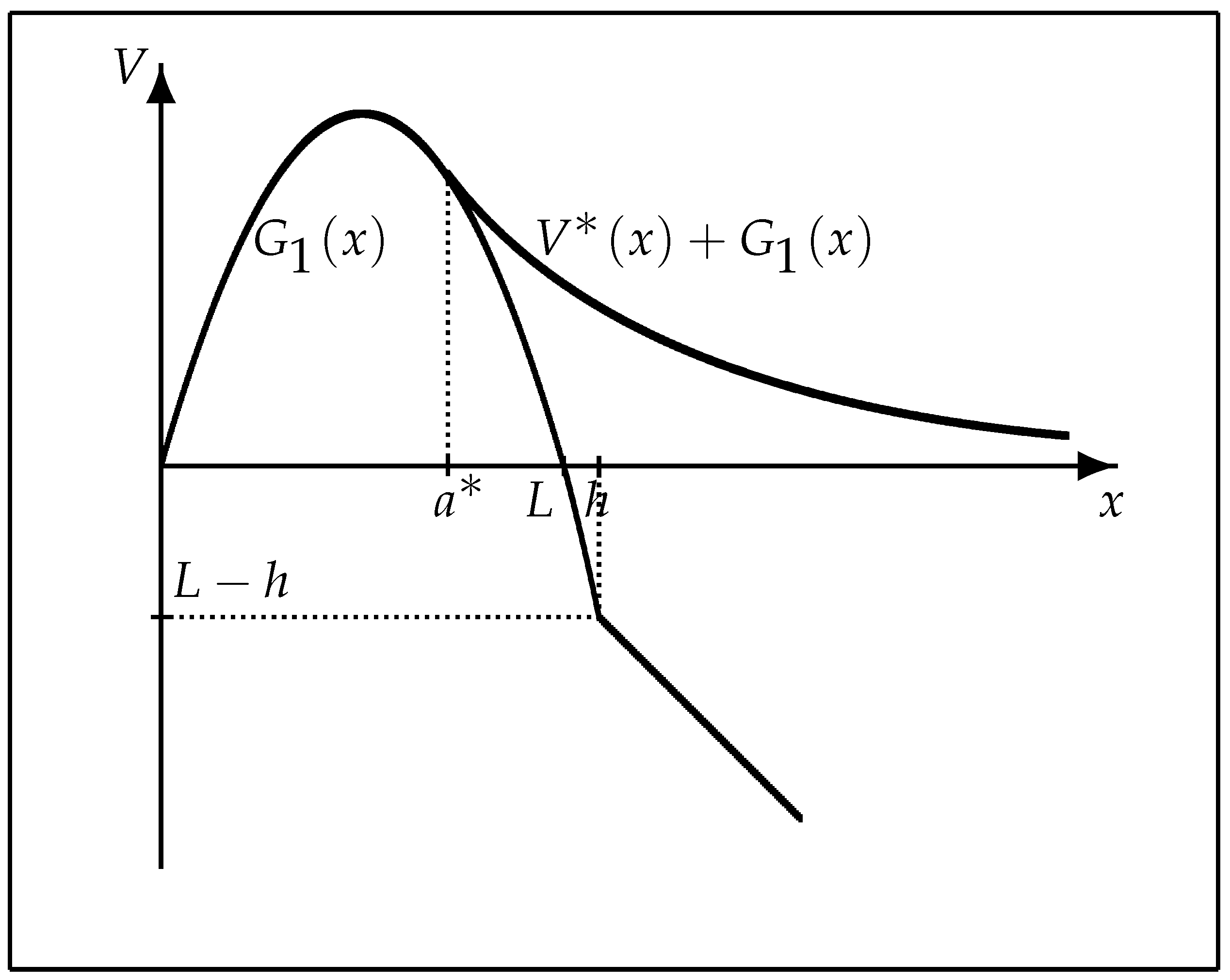
Figure 1.
A computer drawing of the value function .

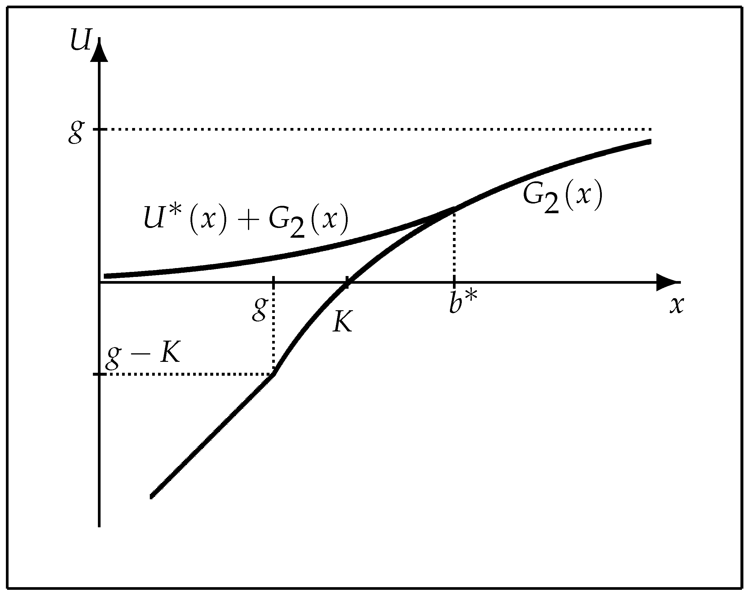
Figure 2.
A computer drawing of the value function .
Publisher’s Note: MDPI stays neutral with regard to jurisdictional claims in published maps and institutional affiliations. |
© 2020 by the authors. Licensee MDPI, Basel, Switzerland. This article is an open access article distributed under the terms and conditions of the Creative Commons Attribution (CC BY) license (http://creativecommons.org/licenses/by/4.0/).
Share and Cite
MDPI and ACS Style
Gapeev, P.V.; Li, L.; Wu, Z. Perpetual American Cancellable Standard Options in Models with Last Passage Times. Algorithms 2021, 14, 3. https://0-doi-org.brum.beds.ac.uk/10.3390/a14010003
AMA Style
Gapeev PV, Li L, Wu Z. Perpetual American Cancellable Standard Options in Models with Last Passage Times. Algorithms. 2021; 14(1):3. https://0-doi-org.brum.beds.ac.uk/10.3390/a14010003
Chicago/Turabian StyleGapeev, Pavel V., Libo Li, and Zhuoshu Wu. 2021. "Perpetual American Cancellable Standard Options in Models with Last Passage Times" Algorithms 14, no. 1: 3. https://0-doi-org.brum.beds.ac.uk/10.3390/a14010003
Note that from the first issue of 2016, this journal uses article numbers instead of page numbers. See further details here.