A Discrete-Continuous Algorithm for Free Flight Planning


Zuse Institute Berlin, Takustraße 7, 14195 Berlin, Germany
*
Author to whom correspondence should be addressed.
†
These authors contributed equally to this work.
Algorithms 2021, 14(1), 4; https://0-doi-org.brum.beds.ac.uk/10.3390/a14010004
Submission received: 30 November 2020
/
Revised: 15 December 2020
/
Accepted: 20 December 2020
/
Published: 25 December 2020
(This article belongs to the Special Issue Algorithms for Shortest Paths in Dynamic and Evolving Networks)
Abstract
:We propose a hybrid discrete-continuous algorithm for flight planning in free flight airspaces. In a first step, our discrete-continuous optimization for enhanced resolution (DisCOptER) method computes a globally optimal approximate flight path on a discretization of the problem using the method. This route initializes a Newton method that converges rapidly to the smooth optimum in a second step. The correctness, accuracy, and complexity of the method are governed by the choice of the crossover point that determines the coarseness of the discretization. We analyze the optimal choice of the crossover point and demonstrate the asymtotic superority of DisCOptER over a purely discrete approach.
Keywords:
shortest path; flight planning; free flight; discrete-continuous algorithm; optimal control; discrete optimizationMSC:
90C35 ; 49M37; 65K10; 65L10; 90C27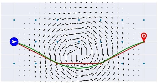
1. Introduction
Flight planning is concerned with the computation of time and fuel efficient flight paths with respect to the weather, see [1] for a comprehensive survey. In particular, wind conditions make a big difference: flying with a headwind of 60 kts increases flight time and fuel consumption of an Airbus A321 by as much as 20% over a tailwind of 60 kts [2]. To exploit this potential, and to mitigate airspace congestion, free flight aircraft routing has been suggested since 1995 [3], and projects to complement, enhance, and finally replace the airway network that is currently used to organize all air traffic are now under way all over the world. Europe is introducing so-called free route airspaces (FRAs), in which one can fly on arbitrary straight lines between defined entry and exit points, and between more and more intermediate points, moving ever closer towards free flight. According to EUROCONTROL, FRA projects are now in place in three quarters of all European airspaces, and, once fully implemented, will save total fuel burn, CO2, and H2O emissions by 1.6–2.3%, which amounts to 3000 tonnes of fuel/day, 10,000 tonnes of CO2/day, €3 million in fuel costs/day, and 500,000 nautical miles/day [4].
The flight planning problem can be seen as a special type of time-dependent shortest path problem. A large number of algorithms has been developed in this general context, including contraction hierarchies, hub labeling, and arc flags for route planing in road networks, see [5,6] for surveys, RAPTOR, transfer patterns, and connection scan for journey planning in public transport networks [6], the isochrones method and dynamic programming for ship weather routing [7], and sampling-based algorithms like rapidly exploring random graphs and trees (RRTs), probabilistic road maps (PRMs), artificial potential fields, as well as graph-based algorithms such as , , theta*, etc. for robot path planning [8]. The variety of these methods reflects the different characteristics of the respective problems.
The best flight planning methods are currently super-fast /Dijkstra algorithms that employ efficient problem specific speed-up techniques such as cost projection [9], super-optimal wind [10], and active constraint propagation [11]. They can find globally optimal solutions of basic problem variants on the world wide airway network with its 100,000 nodes and 600,000–700,000 edges within milliseconds. methods can in principle be extended to deal with FRAs or free flight by excessive graph augmentation, but only up to a certain point, when the graphs become too large and dense.
On the other hand, numerical methods of optimal control are able to compute optimal free flight trajectories to high precision with great efficiency, either with indirect methods based on Pontryagin’s maximum principle [12,13,14,15], or by direct methods using a collocation discretization to reformulate the problem as a nonlinear program (NLP) [16,17]. These methods compute a smooth trajectory independently of any a priori network discretization, i.e., the desired free flight path. The computational complexity of solving the optimality systems by Newton’s method is asymptotically much smaller than for graph discretizations. If measured in terms of accuracy, higher order discretizations of the underlying ordinary differential equations exhibit even larger asymptotic gains. The drawback is that continuous optimal control methods converge only locally, and towards any local optimum, without providing any guarantee of global optimality. Approaches to compute globally optimal solutions to optimal control problems include global optimal control [18], mixed-integer optimal control [19], and various heuristics [20]. Applications to flight planning exist, but consider only very small networks [21] or vertical profiles [22].
We propose in this paper the novel hybrid algorithm discrete-continuous optimization for enhanced resolution (DisCOptER) that combines the strengths of discrete and continuous approaches to flight planning, and provide a numerical study of its efficiency and accuracy. The discrete component of our method provides global optimality, the continuous component high accuracy and asymptotic efficiency. The idea of the method is to do a discrete search for a global optimum on a coarse, approximate, artificial network, and to use the resulting approximate solution to initialize a Newton method for the solution of a continuous optimal control problem. The correctness and effectiveness of this strategy depends on the choice of the crossover point between the discrete and the continuous part of the algorithm. The network for the discrete part must be coarse enough to be searched efficiently, and fine enough to guarantee sufficient proximity to the continuous optimum, such that a subsequent Newton iteration will converge to the latter. Clearly, the convergence radius of the continuous method strongly depends on the gradients of the wind field and affects, together with the approximation error associated with the graph, the computational complexity of both methods. We shall show that this idea is ideally suited for free flight settings.
Our aim in this paper is to demonstrate the potential of combining discrete and continuous optimization methods for the solution of problems that involve space or time discretizations. The goal is to achieve global optimality and rapid convergence at the same time. The model that we consider is simple, and the special characteristics of flight planning have left their imprint. The basic idea, however, should, with suitable modifications, be applicable to various problems of similar nature. In this vein, our paper intends to give a first indication of the usefulness of such approaches.
The paper is structured as follows. Section 2.1, Section 2.2, Section 2.3 describe the free flight problem that we consider. The DisCOptER algorithm is introduced in Section 2.4 including error and complexity estimates. Finally, Section 3 provides a computational study and analyzes the choice of the switch over point.
2. Materials and Methods
2.1. Free Flight Planning
We consider in this paper an idealized version of the flight planning problem in 2D Euclidean space subject to a stationary wind field. We want to compute a flight path that connects an origin and a destination ; the path parameter measures the flight time. The path is influenced by a smooth field of stationary wind of bounded magnitude . Flying at an airspeed of constant magnitude , the aircraft arrives at time , which we seek to minimize. Our setting is chosen for ease of exposition, but our method carries over to more complex 3D and/or time dependent versions, or other objectives, in particular, minimization of fuel consumption.
2.2. Continuous Approach: Optimal Control
In free flight, the flight path is not restricted to a predefined airway network of waypoints and segments. Instead, any Lipschitz-continuous path , with almost everywhere, connecting origin and destination , is a valid trajectory. Among those, we shall find one of minimal flight duration T. This classic of optimal control is known as Zermelo’s navigation problem [23].
In order to formulate the problem over a fixed interval independent of the actual flight duration, we scale time by as usual in free end time problems and arrive at the following optimal control problem for the flight duration , the flight path , and the airspeed :
Here, the constraint maps from the primal domain to the image space .
2.2.1. Optimality Conditions
Let us briefly recall the necessary and sufficient optimality conditions for the optimal control problem (1). With and , the Lagrangian is defined as
If z is a (local) minimizer, the necessary first order or Karush–Kuhn–Tucker (KKT) condition
and the necessary second order condition
hold [24], since is surjective due to . Moreover, if the KKT conditions (3) are satisfied at z for some and the sufficient second order condition (SSC)
holds for some , then z is a locally unique solution of (1) and stable under perturbations of the problem, e.g., due to sufficiently fine discretization. Let us point out that for wind fields with non-vanishing second derivative, in general there is no closed form solution of the necessary conditions (3), such that solutions must be approximated numerically.
Approaches to computing solutions of (1) generally fall into two classes: indirect methods relying on Pontryagin’s maximum principle [15,25] and direct methods based on discretization of the minimization problem (1) [26,27]. Indirect methods lead to a boundary value problem for state x and adjoint state together with a pointwise optimality condition for the control v, which can be solved by shooting type methods, collocation, or spectral discretization approaches [28,29]. The discretization of direct methods, usually by collocation or spectral methods, translates the optimal control problem in a finite dimensional nonlinear program to be solved by corresponding optimization problems [16,17,30]. While indirect methods using multiple shooting lead to smaller problem sizes than direct methods based on collocation in particular for high accuracy requirements, the latter are widely seen as being easier to implement and use, in particular in the presence of state constraints.
In both approaches, Newton-type methods for solving either discretized boundary value problems or nonlinear programming problems converge in general only locally towards a close-by minimizer. Thus, sufficiently good initial iterates need to be provided. The domain of convergence can be extended using line search methods or trust region methods, but without guarantee of global optimality. Special care has to be taken in the case of non-convex problems, since the Newton direction need not be a descent direction if far away from a minimizer satisfying the sufficient second order conditions. Convexification, truncation of iterative solvers [31,32,33], or solvers for non-convex quadratic programs can be used to address this.
2.2.2. Collocation Discretization
Exemplarily, we consider a discretize-then-optimize approach based on direct collocation with the midpoint rule. Let be a time grid, and the piecewise linear and piecewise constant ansatz spaces for positions and velocities, respectively. We discretize (1) by looking for solutions and and require the state equation to be satisfied only at the interval midpoints for . Representing by its nodal values and by its midpoint values , we obtain the large nonlinear program
2.2.3. Discretization Error
The discretization error introduced by the midpoint rule is well-known to be of second order. For given and there is some constant independent of v such that
where is the mesh width, see, e.g., [34]. This translates into a corresponding error in the objective, i.e., the flight time T. Different goal-oriented error concepts have been investigated [35,36] for equality constrained optimal control problems. The excess in actual flight time when the computed path is implemented depends quadratically on the path deviation , and is therefore of order . In any case, the error depends directly on the mesh width , which we therefore use as a coarse but simple qualitative measure of accuracy.
2.2.4. Newton-KKT Solver
Analogous to the continuous Lagrangian (2), we may formulate its discretized counterpart
and the corresponding necessary first order optimality condition
Writing , this can be solved using Newton’s method by computing
For smooth wind fields, there is some related to an affine invariant Lipschitz constant of , such that
holds [37]. Thus, Newton’s method converges quadratically if started sufficiently close to a locally unique solution point , i.e., if . This convergence radius is in general mesh-independent [37,38], and does not depend on the final accuracy in terms of mesh width , but only on problem parameters such as derivatives of the wind w.
2.2.5. Time Complexity
The run time of the Newton-KKT solver is determined by the number of steps and the cost of each step. The computational effort of a Newton step is dominated by the cost of solving the linear equation (8). Due to the ODE structure, is an arrow-shaped matrix with band width independent of . Assuming quasi-uniform meshes, i.e., there is a generic constant such that , this structure allows for an efficient solution in time using direct band solvers.
Starting sufficiently close to the solution, say , allows to bound the truncation error by linear convergence as
which is of course rather pessimistic. A tolerance of to match the discretization error is therefore reached after at most iterations. Thus, the overall complexity in terms of mesh width is
Remark 1.
If an inexact Newton method based on a geometrically refined sequence of meshes with mesh width for some and is used, the number of iterations is determined by the linear convergence of the collocation discretization, while the truncation error is quickly diminished by the quadratic convergence of Newton’s method [37]. Since the effort per Newton step grows geometrically to its final value, the complexity reduces to
provided the initial error is sufficiently small, i.e., .
2.3. Discrete Approach: Shortest Paths in Airway Networks
If flight paths are restricted to a predefined airway network of waypoints and segments, flight planning becomes a special kind of shortest path problem on a digraph. Let be a finite set of waypoints including and , and a set of arcs such that is a strongly connected directed graph. A discrete flight path is a finite sequence of waypoints with for , connecting with . We denote the set of all flight paths by P. The total flight duration for a path is given in terms of the flight duration for an arc by
The travel time on the arc can be computed from the local ground speed
at and the constant airspeed by solving the quadratic equation
This yields
and thus
The discrete optimization problem to be solved is now
2.3.1. Graph Construction
Discrete approaches to (flight) path planning fall into two classes. The first class are sampling-based algorithms. They construct the search graph by some kind of sampling during the execution of the shortest path algorithm, which is usually an -method. This class includes rapidly exploring random trees (RRT) and graph (RRG) algorithms, that are often used in robot path planning [8]. There are versions that guarantee convergence to a global optimum with probability one [39], however, although undoubtedly often extremely efficient in practice, these methods do not provide a priori error bounds or complexity estimates.
The second class are graph-based algorithms, that take the search graph as an input. Impressive super-fast performance in practice, and also theoretically for special classes of graphs, has been achieved by making use of preprocessing as well as sophisticated data structures. However, “proving better running time bounds than those of Dijkstra’s algorithm is unlikely for general graphs” [6]. In many applications, including traditional flight plannning on airway networks, the search graph is canonical. In applications involving space and time discretization, like in free flight, graph construction is a degree of freedom. Using an appropriate discretization, a priori bounds on the runtime and the accuracy of the solutions can be derived. This is the approach that we take.
We cover free flight zones with “locally densely” connected digraphs, i.e., digraphs with a certain density of vertices and arcs.
Definition 1.
A digraph is said to be -dense in a convex set for some , if it satisfies the following conditions:
- 1.
- containment:
- 2.
- vertex density:
- 3.
- arc density: .
We call h the vertex density and the connectivity radius of an -dense graph.
With this definition, and hold. Furthermore, it is easy to see that this graph structure implies that G is strongly connected and therefore P is nonempty, i.e., a path from to exists.
2.3.2. Discretization Error
Similar to the collocation error (6), the error due to graph discretization depends on the vertex density h and the connectivity radius . We restrict our exposition in this paper to a plausible argument for the error order in terms of h and l and refer the reader to [40] for rigorous error bounds of the same orders.
Spatial deviation due to vertex spacing is bounded by , while the linear interpolation error depending on the curvature of the continuous optimal path is bounded by , as illustrated in Figure 1a. Together, the deviation measured as pointwise normal distance is bounded by . As mentioned in Section 2.2 above, this translates quadratically into a flight time error of order .
Assuming that the path actually contains arcs of length around , this order of error is not only an upper bound, but also the expected error. The existence of arcs of length in the optimal discrete path is likely, as the following argument based on Figure 1b shows. With quasi-uniform vertex spacing, the number of adjacent vertices within a distance is of order , such that the average angle between arcs of length up to , and thus the expected angular deviation between the discrete path and the optimal continuous path is of order . The geometric length difference between the discrete path and the continuous path is of order . The expected length and therefore travel time error induced by angular deviation is smallest if is largest, i.e., arcs of maximum length are to be preferred.
This analysis also implies that the total flight time error is of order and that ensures convergence for .
2.3.3. Shortest Path Algorithm
The state-of-the-art for finding shortest paths in airway networks is the algorithm [10], which extends Dijkstra’s algorithm by a (heuristic) lower bound for the distance of some vertex to the destination in order to prioritize the search. Depending on the tightness of the heuristic bound, can discard a substantial part of the graph and reduce the run time considerably. As a particularly fast and simple heuristic we employ the travel time along a straight line between and , assuming maximum tail wind, i.e.,
Tighter and more complex heuristics exploiting local bounds on the wind have been proposed for flight planning, also for time-dependent wind fields [10].
The travel time for each arc is again calculated via numerical integration of (12) using the same method as for the collocation with a fixed discretization. In order to draw up a fair comparison, we process arcs on the fly and thus eliminate any major preprocessing. This also makes the approach extendible to the time dependent case.
2.3.4. Time Complexity
Using a Fibonacci heap for the priority queue, can be implemented to run in time
where and are the numbers of arcs and vertices, respectively. As outlined above, we may assume . If we—conservatively—assume , the total complexity becomes
2.3.5. Graph Structure
Given the above considerations, we now address the question of which graph structure in terms of h and l is the most efficient, i.e., which structure achieves a minimal error for a given computational budget b or, equivalently, a desired accuracy with minimal effort. Models for computational work and accuracy are
We are hence interested in solving the optimization problem
The constraint yields , which, when inserted into the objective, leads to the unconstrained problem
The necessary optimality condition is a quadratic equation in with solution
Inserting this into the constraint yields . We conclude that graphs of optimal efficiency should follow the law
such that the computational complexity of the discrete optimization can be expressed as
with an associated error of in flight time and of in path approximation.
2.4. DisCOptER Algorithm
Due to their superior angular resolution, arcs of length l will occur in the optimal discrete path, while the length of flight path segments in the collocation solution is around . Hence, we expect the accuracy of continuous and discrete optimization approaches to be comparable if . Obviously, for increasing accuracy , the collocation effort of order grows much slower than the effort of complexity . On the other hand, the collocation approach converges only locally.
We therefore propose a hybrid algorithm that combines the strengths of discrete optimization and optimal control, see Algorithm 1. First, a discrete shortest path of low accuracy is calculated using the algorithm as described in Section 2.3. This is used as initial iterate for solving the KKT system (5) to the desired final accuracy using the ordinary Newton method. Employing linesearch or trust region globalization would enlarge the convergence domain of Newton’s method and allow for coarser graphs to be used, but at the cost of less robust and efficient convergence. In favour of robustness and simplicity, we restrict the attention to the ordinary Newton method.
| Algorithm 1: DisCOptER algorithm |
| Input: , , , Output: approximate solution of (1) with error of order , respectively
|
Algorithms that combine methods from discrete and continuous optimization have been proposed before. A reverse deterministic combination going from continuous to discrete has been proposed in [41] based on dynamic programming principles. Other combinations involve a stochastic discrete stage, like rapidly-exploring random trees (RRT, RRT*) (see, e.g., [42]) or Probabilistic Roadmaps (PRMs) [43] in combination with a second NLP stage. Another approach was taken in [44], where the authors use a combination of and RRT* to find an optimal trajectory. These algorithms reveal remarkable performance when it comes to obstacle avoidance. Since our goal is, however, to develop an algorithm with a priori error estimates and bounded runtime, we do not make use of any stochastic approaches in the DisCOptER algorithm.
2.4.1. Initialization
Let be a shortest path from to in the graph G. Let denote the time at which waypoint is passed, and define the relative passage time . We define a mapping of discrete flight paths to continuous paths by piecewise linear interpolation:
The initial collocation iterate is then obtained by evaluating on the collocation grid and defining the airspeeds
at the interval midpoints .
2.4.2. Complexity
The runtime of this hybrid algorithm is comprised of the runtime of the algorithm (13) and the runtime (10) of the KKT-Newton solver for the collocation system. Provided that the initial iterate based on the discrete solution p is sufficiently close to the continuous optimum, i.e., , Newton’s method converges locally as described by (10). For the path approximation error, we expect , which leads to an overall complexity of
or subject to if an inexact Newton method is used. Both complexity bounds essentially suggest to choose a graph as sparse as possible (), only restricted from above by the accuracy necessary for the Newton-KKT solver to converge locally, i.e., , which is independent of the final accuracy .
3. Results
We validate in this section the effectiveness and the efficiency of our algorithm on a test set of four problems of increasing difficulty. Our aim is to demonstrate that our hybrid approach is asymptotically superior to a purely graph based alternative. We discuss the convergence properties of the method in relation to the choice of the crossover point and its dependence on the minimum required graph density. Based on these results, we evaluated the DisCOptER algorithm for varying graph densities, using the theoretically optimal graph structure of , cf. (14). We will see that—as expected—the best performance was achieved on very sparse graphs. The chapter concludes with a computational comparison of the hybrid algorithm with a purely discrete approach.
3.1. Test Problems
We tested our algorithm on a set of simple, but representative examples that were well suited to demonstrate our method, and not far from real world situations or arguably even more difficult. The instances lived in a square or , and the origin and the destination were and , respectively. All values were chosen dimensionless. The wind fields were constructed in a such a way that the straight line from the origin to the destination was particularly unfavorable. The wind speed was limited to , which was rather strong, but not unrealistic. Even though not formally required, the graph nodes were positioned on a uniform Cartesian grid, such that the diagonal distance of two adjacent nodes was . For the sake of simplicity the graph structure will be described based on the node spacing in x-direction . This directly defined by (14).
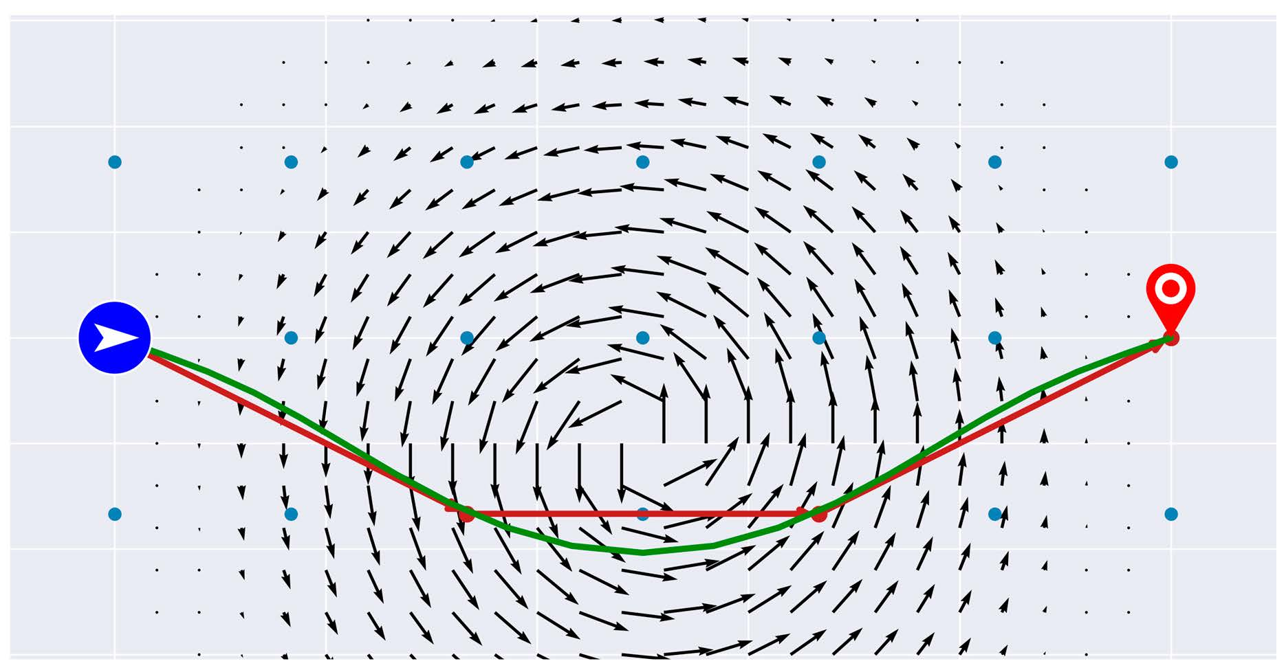
In the first test problem (a), the wind field was a laminar flow of opposing parallel currents, namely,
with , see Figure 2; a similar problem is discussed in [45]. Due to its simplicity, this problem had only one distinct minimum, a property that we make use of in the next section.
In problems (b)–(d), the wind w was the sum of an increasing number of vortices , each of which was described by
where s is the spin of the vortex (: counter-clockwise, : clockwise), is the distance from the vortex center , is the angle with respect to the center and the x-axis with and the absolute vortex wind speed is a function of r and the vortex radius R:
Problem (b) involved one large vortex with at , see Figure 3. This caused Newton’s method to converge to a suboptimal trajectory (above the vortex) if initialized with the straight trajectory. That was the case if the DisCOptER algorithm was used with a minimally sparse graph with (see Figure 3, middle). We observed that the discrete shortest path passed below the vortex for any . From there the globally optimal solution shown in the Figure 3 (left 3), was found for .
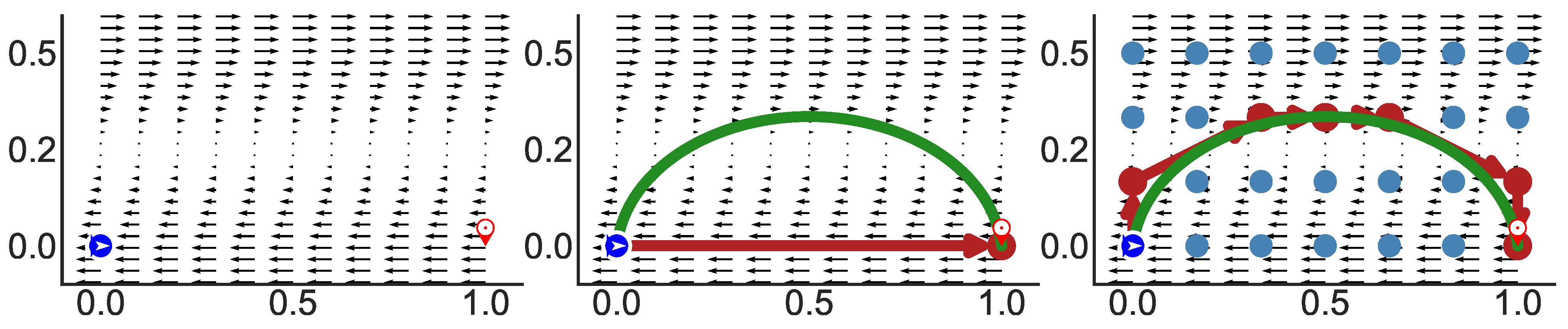
Problem (c) involved 15 vortices with . One was centered at , the others were regularly aligned as seen in Figure 4. Vortices with positive spin (clockwise) were colored green, vortices with negative spin (anti-clockwise) were colored red. Due to the turbulence of this wind field, a plain application of Newton’s method was not guaranteed to converge. As an example, (Figure 4, left 2) shows again the result with the trivial initialization. Further there are several local minima, Figure 4 (left 3 and 4) show two of them. A relatively high graph density () was required to find the globally optimal trajectory (see Figure 4, left 5).
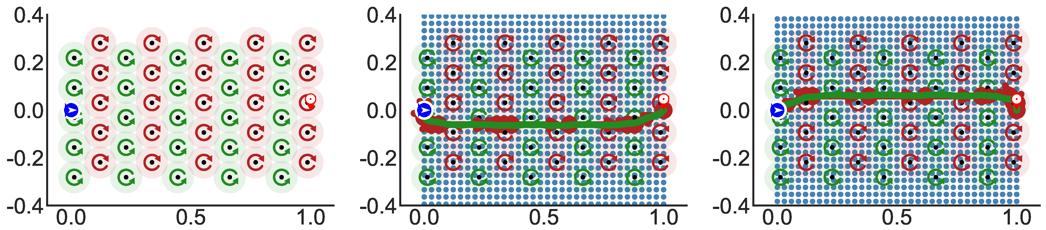
Problem (d) involved 50 regularly aligned vortices of radius (Figure 5). This was clearly an exaggeration, and no commercial plane would ever try to traverse a wind field like this. We used the instance to show that the proposed algorithm outperformed existing methods even under the most adverse conditions. In fact, the high level of non-convexity exacerbated the situation regarding the convergence of Newton’s method. Note that the magnitude of derivatives of (18) was coupled directly to the vortex radius. With the vortices here were half as large as in the previous example. In turn, the first and second order derivatives were 2 and 4 times larger, respectively. Consequently, a quite dense graph with was required to make Newton’s method converge reliably. Note that this wind field was point-symmetric with respect to , which allowed for two equivalent global optima (see Figure 5, left 2 and 3). It was a priori not obvious which one would be found. This depended on the discrete optimum.
3.2. Computational Complexity
Before discussing the DisCOptER algorithm we validated that the optimal control methods were asymptotically more efficient than a purely graph-based approach. This could be investigated only for the first test problem. Due to the simplicity of this wind field, Newton’s method converged from a trivial initialization, i.e., the straight line from to . On the other hand, discrete flight paths were calculated with varying accuracy, that is, with varying l, which is, according to Section 2.3.2, a measure for the accuracy of the calculated path. For the sake of consistency, we indicate the accuracy of the continuous solution by , where L is the path length. Figure 6 clearly confirms the estimated time complexities of for the discrete approach (see Equation (13)) and for the continuous approach (see Equation (10)).
3.3. Minimum Graph Requirements
Figure 7 shows the runtime of the DisCOptER algorithm for various graph parameters . Some key observations could be made for all four test problems. Towards the top right of each figure the graph density increased, which came with an increased runtime dictated by the graph searching part of the algorithm. The black dashed line represents the theoretically optimal graph structure , cf. (14); it is shown for orientation as the results in the following sections were computed with this setting.
From left to right the wind fields became increasingly more non-convex. As these plots reveal, this came with generally higher runtimes, but more importantly with a region of low graph densities where the algorithm converged either to a local minimum or not at all (gray areas). As discussed before, this was not an issue in case (a) since this problem was convex and Newton’s method converged even from a trivial initialization. Even in case (b) we found that a graph with was good enough such that we found the optimal flight path (only one additional column of nodes between start and destination was required). This outcome is not visible here due to the limited resolution of the plot. The convergence problem became all the more apparent with instances (c) and (d). In both cases a good number of local minima existed, each of which had a rather small radius of convergence such that Newton’s method failed if not initialized with sufficient accuracy. Especially in case (d) we saw a patchwork of runs that converged presumably by chance in an unpredictable way. Some of this might be compensated by globalization techniques and an explicit treatment of non-convexity, which, however, would affect the efficiency of Newton’s method. In order to provide reliable results, we need to use a graph density of at least and for case (c) and (d), respectively.
Interestingly, the node distance h appeared to have a much stronger effect on the convergence than the connectedness width l. This might be explained to some extent in terms of the distance and angular error (cf. Section 2.3.2). Low l decreased the angular resolution and thus induced an increased angular error. The discrete flight path then tended to zig-zag along the optimum. This could easily be smoothed by Newton’s method. However, if the discrete flight path was parallely offset from the optimum (distance error due to large node distance h), it might quickly leave the convergence radius of Newton’s method.
3.4. Optimal Crossover Point
In Section 2.3.2 we derived as the optimal graph structure, cf. (14). Using this setting and sampling over various graph densities for the test problems led to the results presented in Figure 8. Obviously, an increased graph density came with a computationally more expensive graph searching task (pink, top, cf. (15)). In turn the NLP part of the algorithm (green, bottom) becomes cheaper following (10), since the initial guess gets closer to the optimum. From test problem a) it can be seen that the best performance was achieved—independently of the overall accuracy —with a relatively low graph density of , where the graph search was still negligibly cheap but the graph was already dense enough for Newton’s method to converge with only one iteration. The exact numbers depended strongly on implementation details. We do not claim to have an optimal realization of either part of the algorithm. The trend towards low graph densities, however, was confirmed by the following examples.
As it turned out, the lower bound on the required graph density imposed by the non-convexity of the wind field was the more important criterion. Looking at examples (c) and (d), where we excluded the area that we identified as not trustworthy in the previous section, we concluded that we want the graph to be as sparse as possible and only as dense as necessary.
3.5. Computational Complexity
We finally showed that globally optimal shortest paths could be calculated more efficiently using the proposed DisCOptER algorithm than with a purely graph based approach, see Figure 9. In the previous section we showed that the algorithm performed best if the graph was chosen rather sparse while respecting the problem-specific minimum density. Consequently, the calculation of the discrete solution was relatively cheap and we could benefit from the computational efficiency of Newton’s algorithm. We can also confirm that the time complexity of the DisCOptER Algorithm is , see Equation (17), and that the time complexity of the purely graph-based approach is , see (13).
4. Conclusions
In this paper we presented the novel DisCOptER algorithm to calculate flight paths in free flight airspaces utilizing a combination of discrete and continuous optimization. We demonstrated that the achieved efficiency is asymptotically much better than the conventional purely discrete alternative. Even though the algorithm was described for the static two-dimensional case it is also strongly promising for more complex cases, to which it can directly be transferred.
Our study also reveals a need for more theoretical analysis of the problem. In order to design a one-shot algorithm with theoretical efficiency guarantees, a priori error estimates allowing the determination of a minimum required crossover graph density is needed. This will of course depend mainly on the characteristics of the wind field including first and second order derivatives. On the other hand, a posteriori error estimates and adaptive coarse-to-fine graph refinement strategies will be necessary for robustness and efficiency in practice. We investigate some of these questions in [40].
Author Contributions
Conceptualization, R.B. and M.W.; methodology, M.W.; software, F.D.; validation, F.D.; formal analysis, M.W.; investigation, F.D. and M.W.; resources, R.B., F.D. and M.W.; data curation, F.D.; writing—original draft preparation, F.D. and M.W.; writing—review and editing, R.B.; visualization, F.D.; supervision, R.B.; project administration, R.B. and M.W.; funding acquisition, R.B. and M.W. All authors have read and agreed to the published version of the manuscript.
Funding
This research was funded by the DFG Research Center of Excellence MATH+ – Berlin Mathematics Research Center, Project AA3-3.
Conflicts of Interest
The authors declare no conflict of interest.
References
- Stojković, S.E.K.S.S.A.G.; Stojković, M. Quantitative Problem Solving Methods in the Airline Industry; Springer: Berlin/Heidelberg, Germany, 2011; Chapter 6—Operations; pp. 283–383. [Google Scholar]
- Airbus Industries. Getting to Grips with Fuel Economy. Issue 4. 2004. Available online: https://ansperformance.eu/library/airbus-fuel-economy.pdf (accessed on 24 December 2020).
- Radio Technical Commission for Aeronautics. Final Report of RTCA Task Force 3 Free Flight Implementation; RTCA: Washington, DC, USA, 1995. [Google Scholar]
- Jelinek, F.; Carlier, S.; Smith, J.; Quesne, A. The EUR RVSM Implementation ProjectEnvironmental Benefit AnalysisEEC/ENV/ 2002/008. Technical Report. 2003. Available online: https://www.eurocontrol.int/eec/gallery/content/public/document/eec/report/2002/023_RVSM_Implementation_Project.pdf (accessed on 24 December 2020).
- Delling, D.; Wagner, D. Time-Dependent Route Planning. In Robust and Online Large-Scale Optimization: Models and Techniques for Transportation Systems; Ahuja, R.K., Möhring, R.H., Zaroliagis, C.D., Eds.; Springer: Berlin/Heidelberg, Germany, 2009; pp. 207–230. [Google Scholar] [CrossRef] [Green Version]
- Bast, H.; Delling, D.; Goldberg, A.; Müller-Hannemann, M.; Pajor, T.; Sanders, P.; Wagner, D.; Werneck, R.F. Route Planning in Transportation Networks. 2015. Available online: https://arxiv.org/pdf/1504.05140.pdf (accessed on 24 December 2020).
- Zis, T.P.; Psaraftis, H.N.; Ding, L. Ship weather routing: A taxonomy and survey. Ocean Eng. 2020, 213, 107697. [Google Scholar] [CrossRef]
- Yang, L.; Qi, J.; Song, D.; Xiao, J.; Han, J.; Xia, Y. Survey of Robot 3D Path Planning Algorithms. J. Control Sci. Eng. 2016, 2016, 1687–5249. [Google Scholar] [CrossRef] [Green Version]
- Blanco, M.; Borndörfer, R.; Hoang, N.D.; De las Casas, A.K.P.M.; Schlechte, T.; Schlobach, S. Cost projection methods for the shortest path problem with crossing costs. In Proceedings of the 17th Workshop on Algorithmic Approaches for Transportation Modelling, Optimization, and Systems (ATMOS 2017), Vienna, Austria, 7–8 September 2017; Volume 59. [Google Scholar]
- Blanco, M.; Borndörfer, R.; Hoang, N.D.; Kaier, A.; Schienle, A.; Schlechte, T.; Schlobach, S. Solving time dependent shortest path problems on airway networks using super-optimal wind. In Proceedings of the 16th Workshop on Algorithmic Approaches for Transportation Modelling, Optimization, and Systems (ATMOS 2016), Aarhus, Denmark, 25 August 2016. Schloss Dagstuhl-Leibniz-Zentrum für Informatik. [Google Scholar]
- Larsen, K.; Knudsen, A.; Chiarandini, M. Constraint handling in flight planning. In Principles and Practice of Constraint Programming; Lecture Notes in Computer Science; Beck, J., Ed.; Springer: Cham, Switzerland, 2017; Volume 10416, pp. 354–369. [Google Scholar]
- Marchidan, A.; Bakolas, E. Numerical Techniques for Minimum-Time Routing on a Sphere with Realistic Winds. Am. Inst. Aeronaut. Astronaut. 2016, 39, 188–193. [Google Scholar] [CrossRef] [Green Version]
- Jardin, M.R.; Bryson, A.E. Methods for computing minimum-time paths in strong winds. J. Guid. Control Dyn. 2012, 35, 165–171. [Google Scholar] [CrossRef]
- McDonald, J.A.; Zhao, Y. Time benefits of free-flight for a commercial aircraft. In Proceedings of the AIAA Guidance Navigation & Control Conference, Dever, CO, USA, 14–17 August 2000. [Google Scholar]
- Von Stryk, O.; Bulirsch, R. Direct and indirect methods for trajectory optimization. Ann. Oper. Res. 1992, 37, 357–373. [Google Scholar] [CrossRef]
- Betts, J.; Cramer, E. Application of direct transcription to commercial aircraft trajectory optimization. J. Guid. Contr. Dyn. 1995, 18, 151–159. [Google Scholar] [CrossRef]
- García-Heras, J.; Soler, M.; Sáez, F.J. A Comparison of Optimal Control Methods for Minimum Fuel Cruise at Constant Altitude and Course with Fixed Arrival Time. Procedia Eng. 2014, 80, 231–244. [Google Scholar] [CrossRef] [Green Version]
- Diedam, H.; Sager, S. Global optimal control with the direct multiple shooting method. Optim. Control Appl. Meth. 2017, 39, 1–22. [Google Scholar] [CrossRef]
- Sager, S.; Reinelt, G.; Bock, H. Direct Methods with Maximal Lower Bound for Mixed-Integer Optimal Control Problems. Math. Program. 2009, 118, 109–149. [Google Scholar] [CrossRef]
- Rao, A. A Survey of Numerical Methods for Optimal Control. Adv. Astronaut. Sci. 2010, 135, 497–528. [Google Scholar]
- Bonami, P.; Olivares, A.; Soler, M.; Staffetti, E. Multiphase mixed-integer optimal control approach to aircraft trajectory optimization. J. Guid. Control Dyn. 2013, 36, 1267–1277. [Google Scholar] [CrossRef] [Green Version]
- Moreno, L.; Fügenschuh, A.; Kaier, A.; Schlobach, S. A Nonlinear Model for Vertical Free-Flight Trajectory Planning. In Operations Research Proceedings; Springer: Cham, Switzerland, 2018; pp. 445–450. [Google Scholar] [CrossRef]
- Zermelo, E. Über das Navigationsproblem bei ruhender oder veränderlicher Windverteilung. ZAMM Z. Angew. Math. Mech. 1931, 11, 114–124. [Google Scholar] [CrossRef]
- Maurer, H.; Zowe, J. First and second-order necessary and sufficient optimality conditions for infinite-dimensional programming problems. Math. Program. 1979, 16, 98–110. [Google Scholar] [CrossRef]
- Pontrjagin, L.; Boltyansky, V.; Gamkrelidze, V.; Mischenko, E. Mathematical Theory of Optimal Processes; Wiley-Interscience: New York, NY, USA, 1962. [Google Scholar]
- Betts, J.T. Survey of Numerical Methods for Trajectory Optimization. J. Guid. Control. Dyn. 1998, 21, 193–207. [Google Scholar] [CrossRef]
- Hargraves, C.; Paris, S. Direct trajectory optimization using nonlinear programming and collocation. J. Guid. Control Dyn. 1987, 10, 338–342. [Google Scholar] [CrossRef]
- Fahroo, F.; Ross, I.M. Direct Trajectory Optimization by a Chebyshev Pseudospectral Method. J. Guid. Control Dyn. 2002, 25, 160–166. [Google Scholar] [CrossRef] [Green Version]
- Ascher, U.; Mattheij, R.; Russell, R. Numerical Solution of Boundary Value Problems for Ordinary Differential Equations; Prentice Hall: Upper Saddle River, NJ, USA, 1988. [Google Scholar]
- Hagelauer, P.; Mora-Camino, F. A soft dynamic programming approach for on-line aircraft 4D-trajectory optimization. Eur. J. Oper. Res. 1998, 107, 87–95. [Google Scholar] [CrossRef] [Green Version]
- Steihaug, T. The conjugate gradient method and trust regions in large scale optimization. SIAM J. Numer. Anal. 1983, 20, 626–637. [Google Scholar] [CrossRef] [Green Version]
- Toint, P. Towards an efficient sparsity exploiting Newton method for minimization. In Sparse Matrices and Their Use; Duff, I., Ed.; Academic Press: Cambridge, MA, USA, 1981; pp. 57–88. [Google Scholar]
- Weiser, M.; Deuflhard, P.; Erdmann, B. Affine conjugate adaptive Newton methods for nonlinear elastomechanics. Optim. Meth. Softw. 2007, 22, 413–431. [Google Scholar] [CrossRef]
- Deuflhard, P.; Bornemann, F. Scientific Computing with Ordinary Differential Equations, 2nd ed.; Texts in Applied Mathematics; Springer: New York, NY, USA, 2002; Volume 42. [Google Scholar]
- Becker, R.; Kapp, H.; Rannacher, R. Adaptive finite element methods for optimal control of partial differential equations: Basic concepts. SIAM J. Control Optim. 2000, 39, 113–132. [Google Scholar] [CrossRef] [Green Version]
- Weiser, M. On goal-oriented adaptivity for elliptic optimal control problems. Optim. Meth. Softw. 2013, 28, 969–992. [Google Scholar] [CrossRef]
- Deuflhard, P. Newton Methods for Nonlinear Problems. Affine Invariance and Adaptive Algorithms; Computational Mathematics; Springer: New York, NY, USA, 2004; Volume 35. [Google Scholar]
- Weiser, M.; Schiela, A.; Deuflhard, P. Asymptotic Mesh Independence of Newton’s Method Revisited. SIAM J. Numer. Anal. 2005, 42, 1830–1845. [Google Scholar] [CrossRef] [Green Version]
- Karaman, S.; Frazzoli, E. Sampling-based algorithms for optimal motion planning. Int. J. Robot. Res. 2011, 30, 846–894. [Google Scholar] [CrossRef]
- Borndörfer, R.; Danecker, F.; Weiser, M. Error Bounds for Free Flight Planning with Locally Connected Airway Networks; Technical Report; Zuse Institute Berlin: Berlin, Germany, in preparation.
- Junge, O.; Osinga, H. A set oriented approach to global optimal control. ESAIM: Contr. Opt. Calc. Var. 2004, 10, 259–270. [Google Scholar] [CrossRef]
- Karatas, T.; Bullo, F. Randomized searches and nonlinear programming in trajectory planning. In Proceedings of the 40th IEEE Conference on Decision and Control (Cat. No.01CH37228), Orlando, FL, USA, 4–7 December 2001; Volume 5, pp. 5032–5037. [Google Scholar] [CrossRef]
- Bouffard, P.; Waslander, S. A Hybrid Randomized/Nonlinear Programming Technique For Small Aerial Vehicle Trajectory Planning in 3D. Plan. Percept. Navig. Intell. Veh. (PPNIV) 2009, 63, 2009. [Google Scholar]
- Brunner, M.; Brüggemann, B.; Schulz, D. Hierarchical Rough Terrain Motion Planning using an Optimal Sampling-Based Method. In Proceedings of the 2013 IEEE International Conference on Robotics and Automation, Karlsruhe, Germany, 6–10 May 2013. [Google Scholar] [CrossRef]
- Techy, L. Optimal navigation in planar time-varying flow: Zermelo’s problem revisited. Intell. Serv. Robot. 2011, 4, 271–283. [Google Scholar] [CrossRef]
Figure 1.
Geometrical error bounds. Blue line: continuous optimal solution. Black line: discrete optimal solution. Gray dots: graph nodes.
Figure 1.
Geometrical error bounds. Blue line: continuous optimal solution. Black line: discrete optimal solution. Gray dots: graph nodes.
Figure 2.
Test problem (a) with , , , . Blue dots: network-graph with and and 6, respectively, red: discrete optimal trajectory, green: continuous optimal trajectory.
Figure 2.
Test problem (a) with , , , . Blue dots: network-graph with and and 6, respectively, red: discrete optimal trajectory, green: continuous optimal trajectory.

Figure 3.
Test problem (b) with counterclockwise spinning vortex centered at , . , , . Blue dots: network graph with and and 6, respectively, red: discrete optimal trajectory, green: continuous optimal trajectory.
Figure 3.
Test problem (b) with counterclockwise spinning vortex centered at , . , , . Blue dots: network graph with and and 6, respectively, red: discrete optimal trajectory, green: continuous optimal trajectory.
Figure 4.
Test problem (c) with 15 vortices, . One is centered at , the others are regularly positioned as seen above. , , . Blue dots: graph with and and 16, respectively, red: discrete optimal trajectory, green: continuous optimal trajectory. Note that the straight trajectory is particularly unfavorable.

Figure 5.
Test problem (d) with 50 vortices (10 columns of 5 vortices each), , regularly positioned. , , . Blue dots: graph with and and 34, respectively, red: discrete optimal trajectory, green: continuous optimal trajectory. Note that, again, the straight trajectory is particularly unfavorable. This problem is point-symmetric w.r.t. . The two shown solutions are equivalent.

Figure 6.
Test case (a). Orange: Discrete-only approach, polynomial trend line of order 6. Purple: Newton-Karush–Kuhn–Tucker (KKT) initialized with straight line, , linear trend line.
Figure 6.
Test case (a). Orange: Discrete-only approach, polynomial trend line of order 6. Purple: Newton-Karush–Kuhn–Tucker (KKT) initialized with straight line, , linear trend line.
Figure 7.
Runtime of the DisCOptER algorithm in seconds. Top right corner: dense graph. Bottom left corner: sparse graph. Gray areas: not converged or converged to local minimum. Black dashed line: . (a–d) refer to the corresponding test problems.
Figure 7.
Runtime of the DisCOptER algorithm in seconds. Top right corner: dense graph. Bottom left corner: sparse graph. Gray areas: not converged or converged to local minimum. Black dashed line: . (a–d) refer to the corresponding test problems.
Figure 8.
Runtimes of the DisCOptER algorithm in seconds, split into the discrete part (pink, top) and the continuous part (green, bottom), sampled with . Constant accuracy . (a–d) refer to the corresponding test problems.
Figure 8.
Runtimes of the DisCOptER algorithm in seconds, split into the discrete part (pink, top) and the continuous part (green, bottom), sampled with . Constant accuracy . (a–d) refer to the corresponding test problems.
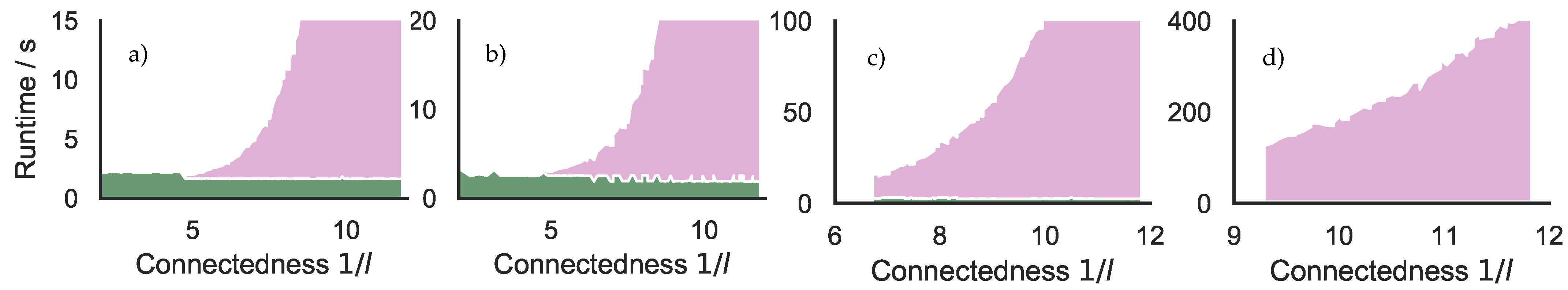
Figure 9.
Minimum runtime in seconds taken experiments similar to Figure 8. Blue: DisCOptER algorithm with , linear trend line. Orange: Purely discrete, polynomial trend line of order 6. (a–d) refer to the corresponding test problems.
Figure 9.
Minimum runtime in seconds taken experiments similar to Figure 8. Blue: DisCOptER algorithm with , linear trend line. Orange: Purely discrete, polynomial trend line of order 6. (a–d) refer to the corresponding test problems.

Publisher’s Note: MDPI stays neutral with regard to jurisdictional claims in published maps and institutional affiliations. |
© 2020 by the authors. Licensee MDPI, Basel, Switzerland. This article is an open access article distributed under the terms and conditions of the Creative Commons Attribution (CC BY) license (http://creativecommons.org/licenses/by/4.0/).
Share and Cite
MDPI and ACS Style
Borndörfer, R.; Danecker, F.; Weiser, M. A Discrete-Continuous Algorithm for Free Flight Planning. Algorithms 2021, 14, 4. https://0-doi-org.brum.beds.ac.uk/10.3390/a14010004
AMA Style
Borndörfer R, Danecker F, Weiser M. A Discrete-Continuous Algorithm for Free Flight Planning. Algorithms. 2021; 14(1):4. https://0-doi-org.brum.beds.ac.uk/10.3390/a14010004
Chicago/Turabian StyleBorndörfer, Ralf, Fabian Danecker, and Martin Weiser. 2021. "A Discrete-Continuous Algorithm for Free Flight Planning" Algorithms 14, no. 1: 4. https://0-doi-org.brum.beds.ac.uk/10.3390/a14010004
Note that from the first issue of 2016, this journal uses article numbers instead of page numbers. See further details here.