A Modified Network-Wide Road Capacity Reliability Analysis Model for Improving Transportation Sustainability

Abstract

Reserve capacity is the core of reliability analysis based on road network capacity. This article optimizes its bi-level programming model: the upper-level model has added service level coefficient and travel time limit, which realizes the unification of capacity and travel time reliability analysis to a certain extent. Stochastic user equilibrium (SUE) model based on origin has been selected as the lower-level model, which added capacity constraints to optimize distribution results, and allows the evaluation of reliability to be continued. Through the SUE model, the iterative step size of the method of successive averages can be optimized to improve the efficiency of the algorithm. After that, the article designs the algorithm flow of reliability analysis based on road network capacity, and verifies the feasibility of the designed algorithm with an example. Finally, combined with the conclusion of reliability analysis, this article puts forward some effective methods to improve the reliability of the urban road network.

1. Introduction

Road network reliability is the application of reliability theory in the field of transportation, which first appeared in system engineering. It is an index to measure the sustainable service of the road network. Reliability analysis based on road network capacity can effectively predict the growth of traffic volume, what the road network can undertake in the future, and it can help to judge whether the traffic can be sustainable. The direction of road network improvement and optimization in the future can be guided by it. The research on road network reliability can be divided into three stages.

The first stage focuses on the road network connectivity reliability, which mainly studies the accessibility from one node to another [1]. In 1989, Iida and Wakabayashi improved it and analyzed the connectivity reliability of the whole network topology [2]. After that, Nicholson used graph theory to analyze connectivity reliability [3]. The calculation method of network connectivity reliability is relatively simple. The topological structure of the road network is abstracted by the idea of series parallel connection, and then the calculation results are obtained [4]. In the case of series connection $P(x)={\displaystyle {\prod }_{i}p(x_i)}$, in parallel $P(x)=1-{\displaystyle {\prod }_i(1-p(x_i))}$, where $p(x_i)$ represents the reliability of the section $i$, $P(x)$ represents the overall reliability of the road network. At the beginning of the study, the connectivity reliability is limited to two states of “pass” and “fail”, with the values of 0 and 1, respectively. In order to better reflect real world traffic operation, the connectivity reliability is extended to [0, 1] [5]. When dealing with complex large-scale networks, it is often necessary to split them into several “small road networks” for analysis. Connectivity reliability is more used to evaluate the reliability after road paralysis caused by disasters [6], which is not applicable to the reliability evaluation of the conventional road network.

The second stage is the development stage, which is represented by travel time reliability analysis. Asakura used the probability index to analyze travel time reliability [7], and then Iida, Haitham, Lo et al. deepened and expanded the research on this basis [8,9,10]. Stephen and David obtained the function family based on the total travel time and the matrix of its distribution after obtaining the link flow and travel time by the stochastic user equilibrium (SUE) model, which can realize the reliability analysis based on travel time [11]. From the perspective of the network, Mahmassani analyzed the reliability of the network based on travel time rate [12]. Compared with the connectivity reliability, taking travel demand into the reliability analysis system can more directly reflect the reliability of the road network in use. Generally, it can be divided into path travel time reliability, OD (Origins and Destinations of the network) travel time reliability and system travel time reliability [13]. Taking the path travel time reliability analysis as an example, the actual calculation is the probability that the time used to select the path is less than the travel time threshold, it can be obtained by $P_i=P(t_i\le t_{ik})$, where $t_i$ is the actual travel time of path $i$, $t_{ik}$ is the acceptable threshold, and is $P_i$ the reliability of path $i$. The analysis of this stage focuses on the results of road network allocation, but more consideration is given to the combing of individual paths, and the analysis results cannot directly guide the direction of road network optimization.

The third stage is the improvement stage. Scholars introduced the network capacity into the travel time reliability analysis, and analyzed the reliability through the travel time ratio under congestion and unblocked conditions. Referring to the methods of Aggarwal, Chan and Li, Anthony Chen et al. defined the reliability of road network capacity based on the random allocation model [14,15,16,17]: the probability that the road network successfully meets the demand of OD connection strength, and designed the algorithm based on the Monte Carlo method [18,19]. The model and algorithm in this stage have certain improvement space to make the analysis more accurate and efficient, which will be discussed in the following paper.

Of course, there are also some other research on reliability abroad. For example, Bell and Schmöcker studied encounter reliability [20], Wong and Bell extended reliability to taxi field [21], Lo conducted in-depth study on intersection operation reliability [22], and Jos studied the relationship between public transport reliability and passenger waiting time [23].

This article improves the reliability analysis based on road network capacity. By adding constraints and coefficients to the model, the analysis results are more realistic. At the same time, it solves the situation that the reliability analysis cannot continue in the first “overload” distribution. The algorithm level points out the direction of designing an efficient algorithm. Then, combined with the analysis results, the article puts forward measures and suggestions to improve the reliability of the road network.

2. Model Improvement

The concept of reliability analysis based on road network capacity is proposed on the basis of reserve capacity, that is, the probability that the actual traffic demand level is lower than the maximum reserve capacity. It can be expressed by Equation (1):

$$R=P(\mu \le {\mu }_r),$$

(1)

where $R$ represents the reliability probability of road network capacity, ${\mu }_r$ represents the reserve capacity, $\mu$ represents the growth coefficient of traffic trip level.

When the traffic flow is zero, the section capacity is not “used” and the reliability is “1”; when the traffic demand level exceeds the reserve capacity, the road network is unreliable. Generally, the approximate value of network capacity reliability is obtained by the idea of upper and lower bound approximation, and the calculation formula is as follows:

$${\displaystyle \sum P_{m}Z(m,\mu )}\le R(\mu ,m)\le {\displaystyle \sum P_{m}Z(m,\mu )}+(1-{\displaystyle \sum p_m}),$$

(2)

where $m$ represents the number of states corresponding to different capacity levels, and $Z$ can be calculated by Equation (3):

$$Z(m,\mu )=\{\begin{array}{l}1\hspace{0.17em}\hspace{0.17em}\hspace{0.17em}{\mu }_{rm}\ge \mu \hspace{0.17em}\hspace{0.17em}\\ 0\hspace{0.17em}\hspace{0.17em}\hspace{0.17em}{\mu }_{rm}<\mu \end{array}.$$

(3)

It can be found that the core of road network capacity reliability calculation is reserve capacity calculation, which is generally calculated by bi-level programming model. The upper-level model solves the maximum reserve capacity, and the lower-level model is the traffic flow allocation model (such as SUE model), it can be expressed as Equation (4):

$$\begin{array}{l}UP\hspace{0.17em}\hspace{0.17em}\hspace{0.17em}\hspace{0.17em}\hspace{0.17em}\hspace{0.17em}\hspace{0.17em}\hspace{0.17em}\hspace{0.17em}\hspace{0.17em}\hspace{0.17em}\max \hspace{0.17em}\hspace{0.17em}{\mu }_r\\ \hspace{0.17em}\hspace{0.17em}\hspace{0.17em}\hspace{0.17em}\hspace{0.17em}\hspace{0.17em}\hspace{0.17em}\hspace{0.17em}s.t.\hspace{0.17em}\hspace{0.17em}\hspace{0.17em}\hspace{0.17em}{x}_a({\mu }_{r}q)\le C_a\\ LP\hspace{0.17em}\hspace{0.17em}\hspace{0.17em}\hspace{0.17em}\hspace{0.17em}\hspace{0.17em}\hspace{0.17em}\hspace{0.17em}\hspace{0.17em}\hspace{0.17em}\hspace{0.17em}SUE\hspace{0.17em}\hspace{0.17em}\hspace{0.17em}\hspace{0.17em}\mathrm{model}\end{array}$$

(4)

where $q$ indicates the traffic demand of the road network, $x_a({\mu }_{r}q)$ represents the traffic flow of section $a$, $C_a$ represents the capacity of section $a$.

According to model 4, it can be found that the precondition for the reserve capacity to continue to be solved is that the flow allocated for the first time should not be higher than the link capacity. However, in the case of no constraint, the result of allocation is often overloaded.

2.1. Upper-Level Model Improvement

The reserve capacity coefficient actually reflects the expansion multiple of the basic OD matrix. In the original model (Equation (4)), the constraint condition is that the link flows which have been expanded should be under capacity limits. Considering that when the road service level is lower than a certain value, travelers cannot arrive at the destination in the given time, which is “unreliable”. On the basis of capacity limitation, this article improves the model by adding service level coefficient $\partial$, and the value can be between 0.8–1.0 [24], as shown in Equation (5):

$$\begin{array}{l}\hspace{0.17em}\hspace{0.17em}\hspace{0.17em}\hspace{0.17em}\hspace{0.17em}\hspace{0.17em}\hspace{0.17em}\hspace{0.17em}\max \hspace{0.17em}\hspace{0.17em}{\mu }_r\\ \hspace{0.17em}\hspace{0.17em}\hspace{0.17em}\hspace{0.17em}\hspace{0.17em}\hspace{0.17em}\hspace{0.17em}\hspace{0.17em}s.t.\hspace{0.17em}\hspace{0.17em}\hspace{0.17em}\hspace{0.17em}{x}_a({\mu }_{r}q)\le \partial C_a\end{array}$$

(5)

At the same time, with the increase of traffic flow, the road impedance increases and the travel time of users increases. After the increase to a certain extent (relative to the original travel time), the road network is actually “unreliable” for users. $t_a(q)$ represents the user’s travel time, $\tau$ is defined as the travel time reliability threshold, if possible, it can be comprehensively selected according to the field survey questionnaire. The meaning of other variables and parameters is the same as above, and the model is improved to Equation (6).

$$\begin{array}{l}\hspace{0.17em}\hspace{0.17em}\hspace{0.17em}\hspace{0.17em}\hspace{0.17em}\hspace{0.17em}\hspace{0.17em}\hspace{0.17em}\max \hspace{0.17em}\hspace{0.17em}{\mu }_r\\ \hspace{0.17em}\hspace{0.17em}\hspace{0.17em}\hspace{0.17em}\hspace{0.17em}\hspace{0.17em}\hspace{0.17em}\hspace{0.17em}s.t.\hspace{0.17em}\hspace{0.17em}\hspace{0.17em}\hspace{0.17em}{x}_a({\mu }_{r}q)\le \partial C_a\\ \hspace{0.17em}\hspace{0.17em}\hspace{0.17em}\hspace{0.17em}\hspace{0.17em}\hspace{0.17em}\hspace{0.17em}\hspace{0.17em}\hspace{0.17em}\hspace{0.17em}\hspace{0.17em}\hspace{0.17em}\hspace{0.17em}\hspace{0.17em}\hspace{0.17em}\hspace{0.17em}{t}_a({\mu }_{r}q)\le \tau t_a(q)\end{array}$$

(6)

It can be found that the improvement of the upper-level model is essentially a restriction on the traffic assignment flow. To a certain extent, the reliability analysis of the traffic capacity and travel time can be unified.

2.2. Lower-Level Model Improvement

The lower-level model is the traffic assignment model. In this article, the SUE model based on origin (see model 7) is selected. Compared to the Fisk model [25], the output of this model is the traffic flow from different origins, which can more intuitively reflect the OD connection demand [7], at the same time, this model can optimize the algorithm design and improve the efficiency [26]:

$$\begin{array}{l}\min \hspace{0.17em}Z(x)={\displaystyle \sum _{}{\displaystyle {\int }_0^{x_a}{t}_a(w)dw-\frac{1}{\theta }}}{\displaystyle \sum _{}\{HL(x^o)-HN(x^0)\}},\\ s.t.\hspace{0.17em}\hspace{0.17em}{g}_k(x^o)={\displaystyle \sum _i{x}_{ik}^o-{\displaystyle \sum _j{x}_{kj}^o+{\displaystyle \sum _d{q}_{od}{\delta }_{ok}-q_{od}}}}{\delta }_{dk}=0\hspace{0.17em}\hspace{0.17em},\hspace{0.17em}\\ \hspace{0.17em}\hspace{0.17em}\hspace{0.17em}\hspace{0.17em}\hspace{0.17em}{x}_a={\displaystyle \sum _{}{x}_{ij}^o}\hspace{0.17em},\hspace{0.17em}\hspace{0.17em}\hspace{0.17em}\hspace{0.17em}\hspace{0.17em}{x}_{ij}^o\ge 0\hspace{0.17em}.\end{array}$$

(7)

where $o$ represents the origin of the network, $d$ represents the destination of the network, $i$, $j$, and $k$ represents node of road network, the $x_{ij}^o$ represents the flow of the road section $(i,j)$ from the origin $o$, ${\delta }_{ok}$ and ${\delta }_{dk}$ are switch functions, when $k=o(d)$,${\delta }_{ok}({\delta }_{dk})=1$, else ${\delta }_{ok}({\delta }_{dk})=0$. The meaning of other functions is the same as above paper. The definition of $HL(x^o)$ and $HN(x^o)$ are as follows:

$$\begin{array}{l}HL(x^o)=-{\displaystyle {\sum }_{ij}{x}_{ij}^{o}In{x}_{ij}^o},\\ HN(x^o)=-{\displaystyle {\sum }_j({\displaystyle {\sum }_i{x}_{ij}^o})In({\displaystyle {\sum }_i{x}_{ij}^o})}{\delta }_{dk}.\end{array}$$

Considering that in the real world, the actual road section flow will not exceed the road capacity, and the saturation is “1” under the most congested state. When the congestion reaches a certain degree, users will choose other routes. The model 7 is optimized as follows, and the capacity constraint is added to the constraint conditions:

$$\begin{array}{l}\min Z(x)={\displaystyle \sum _{}{\displaystyle {\int }_0^{x_a}{t}_a(w)dw-\frac{1}{\theta }}}{\displaystyle \sum _{}\{HL(x^o)-HN(x^0)\}},\\ s.t.\hspace{0.17em}\hspace{0.17em}{g}_k(x^o)={\displaystyle \sum _i{x}_{ik}^o-{\displaystyle \sum _j{x}_{kj}^o+{\displaystyle \sum _d{q}_{od}{\delta }_{ok}-q_{od}}}}{\delta }_{dk}=0\hspace{0.17em}\hspace{0.17em}\hspace{0.17em},\\ \hspace{0.17em}\hspace{0.17em}\hspace{0.17em}\hspace{0.17em}\hspace{0.17em}{x}_a={\displaystyle \sum _{}{x}_{ij}^o}\hspace{0.17em},\hspace{0.17em}\hspace{0.17em}\hspace{0.17em}\hspace{0.17em}{x}_{ij}^o\ge 0,\\ \hspace{0.17em}\hspace{0.17em}\hspace{0.17em}\hspace{0.17em}\hspace{0.17em}{x}_a\hspace{0.17em}\le \partial C_a.\end{array}$$

(8)

3. Algorithm Design

3.1. Overall Process Design

According to the previous paper, the core problem of reliability based on road network capacity is actually to obtain the reserve capacity coefficient. By the reserve capacity coefficient and travel demand, the reliability of the road network can be obtained by Equation (2). The overall process of the algorithm design can be as follows:

Step 1: For a given OD matrix, the lower-level SUE model with constraints is solved to obtain the link flow.

Step 2: Construct the sensitivity matrix to obtain the linear programming functions of the link flow and travel time with respect to the given OD matrix, simplify the upper-level model problem, and obtain the ${\mu }_r{}^{(n)}$.

Step 3: After expanding the OD matrix ${\mu }_r{}^{(n)}$ times, repeat steps 1 and 2 to get new ${\mu }_r{}^{(n+1)}$.

Step 4: Convergence judgment. When $\left|{\mu }_r{}^{(n+1)}\ast {\mu }_r{}^{(n)}-{\mu }_r{}^{(n)}\right|\le \epsilon$ (where $\epsilon$ is a very small real number, it can be 0.01) or ${\mu }_r{}^{(n+!)}<1$, the reserve capacity coefficient ${\mu }_r{}^{}=\max ({\mu }_r{}^{(n)}\ast {\mu }_r{}^{(n+1)},\hspace{0.17em}{\mu }_r{}^{(n)})$ is obtained. Otherwise, taking ${\mu }_r{}^{(n)}={\mu }_r{}^{(n)}\ast {\mu }_r{}^{(n+1)}$, repeat the above steps until convergence.

When $\left|{\mu }_r{}^{(n+1)}\ast {\mu }_r{}^{(n)}-{\mu }_r{}^{(n)}\right|\le \epsilon$ (where $\epsilon$ is a very small real number, it can be 0.01), it means that there is no big difference between ${\mu }_r{}^{(n+1)}\ast {\mu }_r{}^{(n)}$ times expansion and ${\mu }_r{}^{(n)}$ times expansion of the given OD matrix. It is approximately considered that the reserve capacity coefficient ${\mu }_r={\mu }_r{}^{(n)}\ast {\mu }_r{}^{(n+1)}$ has been obtained. Or when ${\mu }_r{}^{(n+!)}<1$, it means that the given OD matrix cannot be expended any more, then the reserve capacity coefficient is ${\mu }_r{}^{(n)}$.

Step 5: By comparing the relationship between the reserve capacity and the growth threshold of traffic demand, according to Equation (2), the reliability of the road network can be obtained.

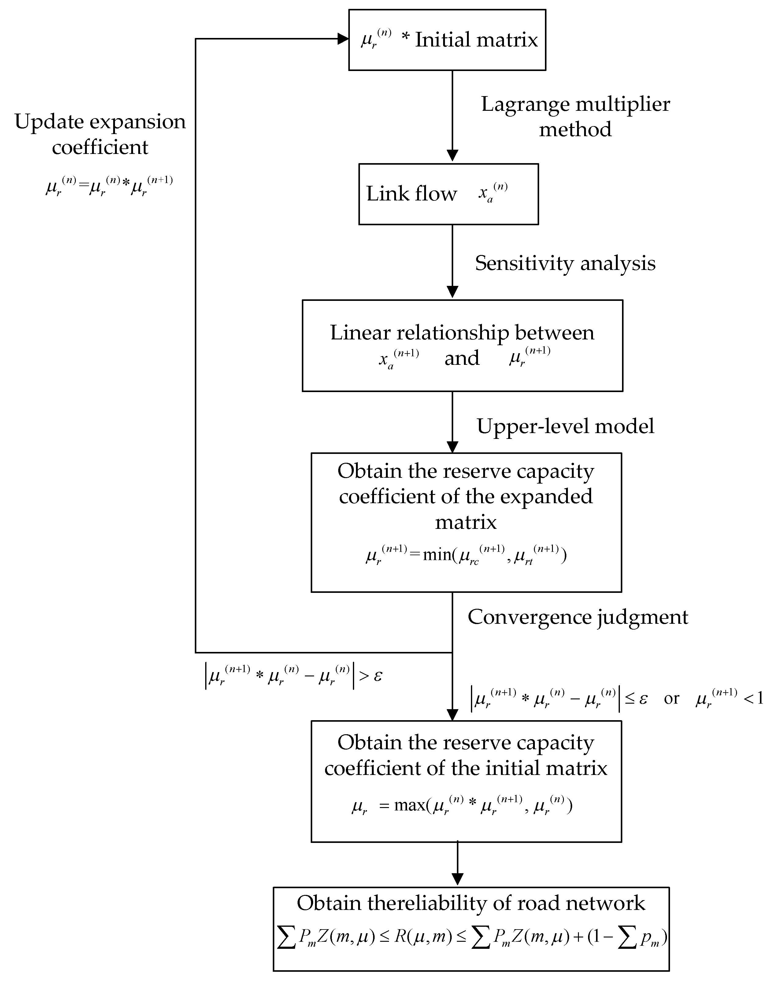
In addition, the flowchart of the algorithm is as shown in Figure 1. Where, at the first time, ${\mu }_r{}^{(1)}=1$, and $n=1,2,\cdots ,m$, $m$ is a positive real number.

3.2. Relative Algorithm

According to the previous reliability analysis process, it can be found that the algorithms involved the SUE problem with constraints and sensitivity analysis problem. To solve the SUE problem with constraints, the penalty algorithm such as the Lagrange multiplier method can be used, and the optimal solutions can be obtained by continuous iteration [27]. Its essence is the design of the traffic assignment algorithm. The sensitivity analysis problem can use the method of mathematical programming, which is relatively simple to get the results.

3.2.1. Optimization of Method of Successive Averages (MSA)

MSA is a traditional algorithm to solve the SUE problem. The general process is as follows:

Step 1: Initialization. The free travel time is taken as the travel impedance to load the traffic, and the initial value is obtained $x^{(1)}$, the iteration count is defined as $\tau =1$.

Step 2: The impedance is updated from the previous section flow as $t_{ij}^{\tau }=t(x_{ij}^{(\tau )})$, and then the auxiliary flow $y^{(\tau )}$ can be obtained by distributing the flow on the basis of the new impedance.

Step 3: Calculating the search direction $d^{(\tau )}$, and the “successive average” movement is carried out as follows:

$$\begin{gathered} d^{(\tau )}=y^{(\tau )}-x^{(\tau )} \\ {x}^{(\tau +1)}=x^{(\tau )}+\frac{1}{\tau }{d}^{(\tau )}. \end{gathered}$$

Step 4: Convergence check. If satisfied, stop, otherwise continue with step 2.

For traffic loading, dial algorithm can be used, which will not be discussed here.

In terms of convergence conditions, in practical application, the number of times can be selected to judge regardless of the convergence situation; the following formula can also be used:

$$\begin{gathered} \frac{\sqrt{{\displaystyle \sum _{ij}({\overline{x}}_{ij}^{\tau +1}-{\overline{x}}_{ij}^{\tau })}}}{{\displaystyle \sum _{ij}{\overline{x}}_{ij}^{\tau }}}\le \phi , \\ {\overline{x}}_{ij}^{\tau }=\frac{1}{n}(x_{ij}^{\tau }+x_{ij}^{\tau -1}+\cdots x_{ij}^{\tau -m+1}), \end{gathered}$$

where $\phi$ can take a minimum constant. $\tau >n$ and $n$ can be taken as $n=3$.

It can be found that the original MSA algorithm does not involve the evaluation of the SUE model, and the step size is “successive average sequence” defined by itself. In self convergence, the speed is very slow, and the accuracy is difficult to guarantee by defining the convergence times. In terms of evaluation function, the SUE model based on origin avoids path enumeration, and can improve the convergence efficiency of MSA. Lee has verified that the efficiency of the improved MSA is higher than the original by the Sioux Fall network and the Barcelona network [28].

Step 1: Initialization. Get the initial solutions $x^{(1)}$, let the count function $\tau =1$.

Step 2: Look for search directions. The auxiliary solution is found to satisfy the sub problem, which is:

$$\begin{gathered} \begin{array}{l}\min \hat{Z}(y)={\displaystyle \sum _{(i,j)\in L}{t}_{ij}\left[x_{ij}^{(\tau )}\right]y_{ij}+}\frac{1}{\theta }{\displaystyle \sum _{o\in O}\left\{{\displaystyle \sum _{(i,j)\in L}{y}_{ij}{}^o}In{y}_{ij}{}^o-{\displaystyle \sum _{j\in N}\left[({\displaystyle \sum _{(i,j)\in L}{y}_{ij}{}^o})In({\displaystyle \sum _{(i,j)\in L}{y}_{ij}{}^o})\right]}\right\}}\\ \hspace{0.17em}\hspace{0.17em}\hspace{0.17em}\hspace{0.17em}\hspace{0.17em}\hspace{0.17em}\hspace{0.17em}\hspace{0.17em}\hspace{0.17em}\hspace{0.17em}\hspace{0.17em}\hspace{0.17em}\hspace{0.17em}\hspace{0.17em}\hspace{0.17em}\hspace{0.17em}\end{array} \\ s.t.{\displaystyle \sum _i{\mathrm{y}}_{ik}^o-{\displaystyle \sum _j{y}_{kj}^o+{\displaystyle \sum _d{q}_{od}{\delta }_{ok}-{\delta }_{dk}{q}_{od}}}}=0, \\ {y}_{ij}={\displaystyle \sum _o{y}_{ij}^o}, \\ {y}_{ij}^o\ge 0. \end{gathered}$$

where $y_{ij}^o$ represents the flow of the road section $(i,j)$ from the origin $o$, and the descent direction can be similar to the original MSA.

Step 3: Convergence check. If the convergence condition is reached, stop. Otherwise, proceed to step 4.

Step 4: Update step size. The solution ${\mathsf{\mu }}^{(\tau )}$ is nonnegative number and satisfies the following conditions:

$$\underset{0\le \mu \le 1}{\min }Z\left[x^{(\tau )}+{\mathsf{\mu }}^{(\tau )}{d}^{(\tau )}\right].$$

Step 5: Move. Get new traffic flow $x^{(\tau +1)}$:

$$x^{(\tau +1)}=x^{(\tau )}+{\mathsf{\mu }}^{(\tau )}{d}^{(\tau )}.$$

Let $\tau =\tau +1$, and go back to step 2.

It can be found that the key of the new optimization algorithm is to solve the sub problem of step 2, where the dial or bell algorithm is used to load. Step 1 can also use travel time of zero flow to load bell second algorithm.

The convergence criterion can be set to the following Equation (9). Compared with the step size of the original MSA, the convergence will be faster:

$$\nabla z{\left[x^{\tau }\right]}^T•\left[y^{\tau }-x^{\tau }\right]\ge -\phi ,$$

(9)

where $\phi$ can take a small real number.

3.2.2. Construction of Sensitivity Equation

The Lagrange multipliers of constraint conditions of model 8 are defined as ${\mu }_k$ and $d_a$, and the original model can be transformed into model 10 [29]:

$$L(x,\mathsf{\mu },d,\mathsf{\epsilon })=Z(x,\mathsf{\epsilon })+{\displaystyle {\sum }_k{\mu }_k}{h}_k(x^o,\mathsf{\epsilon })\hspace{0.17em}-{\displaystyle {\sum }_a{d}_a}{g}_a(x,\mathsf{\epsilon }).$$

(10)

According to the Kuhn–Tucker condition, the equations are obtained:

$$G=\{\begin{array}{l}\nabla L=0\\ d_a{g}_a(x,\mathsf{\epsilon })=0\\ h_k(x^o,\mathsf{\epsilon })=0\end{array}, y(\mathsf{\epsilon })=\left[\begin{array}{l}{x}^o(\mathsf{\epsilon })\\ d(\mathsf{\epsilon })\\ u(\mathsf{\epsilon })\end{array}\right].$$

In the optimal solution, the derivation of the above equations can be obtained as follows:

$$\left[\begin{array}{l}{\nabla }^{2}L\hspace{0.17em}\hspace{0.17em}\hspace{0.17em}\hspace{0.17em}-\nabla g^T\hspace{0.17em}\hspace{0.17em}\hspace{0.17em}\hspace{0.17em}\hspace{0.17em}\nabla h^T\\ d\nabla g\hspace{0.17em}\hspace{0.17em}\mathrm{diag}(g)\hspace{0.17em}\hspace{0.17em}\hspace{0.17em}\hspace{0.17em}\hspace{0.17em}\hspace{0.17em}0\\ \hspace{0.17em}\hspace{0.17em}\nabla h\hspace{0.17em}\hspace{0.17em}\hspace{0.17em}\hspace{0.17em}\hspace{0.17em}\hspace{0.17em}0\hspace{0.17em}\hspace{0.17em}\hspace{0.17em}\hspace{0.17em}\hspace{0.17em}\hspace{0.17em}\hspace{0.17em}\hspace{0.17em}\hspace{0.17em}\hspace{0.17em}0\end{array}\right]{\nabla }_{\mathsf{\epsilon }}y+\left[\begin{array}{l}{\nabla }_{\epsilon x^o}{}^{2}L\\ d{\nabla }_{\epsilon }g\\ \hspace{0.17em}{\nabla }_{\epsilon }h\end{array}\right]=0,$$

where “$\mathrm{diag}$” represents a diagonal matrix with diagonal vectors. In order to simplify the model form, vector matrices $\mathit{M}$ and $\mathit{N}$ are defined:

$$\mathit{M}\equiv \left[\begin{array}{l}{\nabla }^{2}L\hspace{0.17em}\hspace{0.17em}\hspace{0.17em}\hspace{0.17em}-\nabla g^T\hspace{0.17em}\hspace{0.17em}\hspace{0.17em}\hspace{0.17em}\hspace{0.17em}\nabla h^T\\ d\nabla g\hspace{0.17em}\hspace{0.17em}\mathrm{diag}(g)\hspace{0.17em}\hspace{0.17em}\hspace{0.17em}\hspace{0.17em}\hspace{0.17em}\hspace{0.17em}0\\ \hspace{0.17em}\hspace{0.17em}\nabla h\hspace{0.17em}\hspace{0.17em}\hspace{0.17em}\hspace{0.17em}\hspace{0.17em}\hspace{0.17em}0\hspace{0.17em}\hspace{0.17em}\hspace{0.17em}\hspace{0.17em}\hspace{0.17em}\hspace{0.17em}\hspace{0.17em}\hspace{0.17em}\hspace{0.17em}\hspace{0.17em}0\end{array}\right], \mathit{N}\equiv {\left[-{\nabla }_{\epsilon x^o}{}^2{L}^T,\hspace{0.17em}\hspace{0.17em}-d{\nabla }_{\epsilon }{g}^T\hspace{0.17em},\hspace{0.17em}-{\nabla }_{\epsilon }{h}^T\right]}^T.$$

Then, we can get: ${\nabla }_{\epsilon }y={\mathit{M}}^{-1}\mathit{N}$.

From the above formula, combined with Taylor expansion, Equation (11) can be obtained:

$$y\left(\mathbf{\epsilon }\right)=\left[\begin{array}{l}{x}^o(0)\\ d(0)\\ u(0)\end{array}\right]+\left(\mathit{M}{\left(0\right)}^{-1}\mathit{N}\left(0\right)\right)\mathsf{\epsilon }+o\left(\left|\right|\mathsf{\epsilon }\left|\right|\right).$$

(11)

where $\mathsf{\epsilon }$ represents the disturbance of the input variable, $o\left(\left|\right|\mathsf{\epsilon }\left|\right|\right)$ is a real parameter, when $\mathsf{\epsilon }\to 0$, $o\left(\left|\right|\mathsf{\epsilon }\left|\right|\right)\to 0$. After getting a set of initial solutions, a new solution with the change of free flow time or OD demand can be obtained according to Equation (12).

According to Equation (11), the Hessian matrix is obtained:

$${\nabla }^{2}L=\mathrm{diag}{\left({\left(t_{ij}(x_{ij})\right)}_{x_{ij}}\right)}_{ij}-\frac{1}{\theta }\left(\frac{1}{{\displaystyle \sum _m{x}_{mj}^o}}-\frac{1}{x_{ij}^o}{\delta }_{ij,gh}\right).$$

When the section $(g,h)$ equal to the section $(i,j)$, ${\delta }_{ij,gh}=1$, otherwise it is zero. At the same time, according to the Kuhn–Tucker condition, when $x_{ij}\le C_{ij}$, $d_a=0$; when $x_{ij}>C_{ij}$, a penalty algorithm is needed to make the solution approximate the real value, so $g_a(x_{ij})=0$.

According to the above analysis, the vector matrix $\mathit{M}$ and $\mathit{N}$ can be transformed into:

$$\mathit{M}=\left[\begin{array}{l}1\hspace{0.17em}\hspace{0.17em}\hspace{0.17em}\hspace{0.17em}\hspace{0.17em}0\hspace{0.17em}\hspace{0.17em}\hspace{0.17em}\hspace{0.17em}0\hspace{0.17em}\\ 0\hspace{0.17em}\hspace{0.17em}\hspace{0.17em}-d\hspace{0.17em}\hspace{0.17em}\hspace{0.17em}0\\ 0\hspace{0.17em}\hspace{0.17em}\hspace{0.17em}\hspace{0.17em}\hspace{0.17em}0\hspace{0.17em}\hspace{0.17em}\hspace{0.17em}\hspace{0.17em}1\end{array}\right]•\left[\begin{array}{l}{\nabla }^{2}L\hspace{0.17em}\hspace{0.17em}\hspace{0.17em}\hspace{0.17em}-\nabla g^T\hspace{0.17em}\hspace{0.17em}\hspace{0.17em}\hspace{0.17em}\hspace{0.17em}\nabla h^T\\ -\nabla g\hspace{0.17em}\hspace{0.17em}\hspace{0.17em}\hspace{0.17em}\hspace{0.17em}\hspace{0.17em}0\hspace{0.17em}\hspace{0.17em}\hspace{0.17em}\hspace{0.17em}\hspace{0.17em}\hspace{0.17em}\hspace{0.17em}\hspace{0.17em}\hspace{0.17em}\hspace{0.17em}0\\ \hspace{0.17em}\hspace{0.17em}\nabla h\hspace{0.17em}\hspace{0.17em}\hspace{0.17em}\hspace{0.17em}\hspace{0.17em}\hspace{0.17em}0\hspace{0.17em}\hspace{0.17em}\hspace{0.17em}\hspace{0.17em}\hspace{0.17em}\hspace{0.17em}\hspace{0.17em}\hspace{0.17em}\hspace{0.17em}\hspace{0.17em}0\end{array}\right], \mathit{N}=\left[\begin{array}{l}1\hspace{0.17em}\hspace{0.17em}\hspace{0.17em}\hspace{0.17em}\hspace{0.17em}0\hspace{0.17em}\hspace{0.17em}\hspace{0.17em}\hspace{0.17em}0\hspace{0.17em}\\ 0\hspace{0.17em}\hspace{0.17em}\hspace{0.17em}-d\hspace{0.17em}\hspace{0.17em}\hspace{0.17em}0\\ 0\hspace{0.17em}\hspace{0.17em}\hspace{0.17em}\hspace{0.17em}\hspace{0.17em}0\hspace{0.17em}\hspace{0.17em}\hspace{0.17em}\hspace{0.17em}1\end{array}\right]•\left[\begin{array}{l}-{\nabla }_{\epsilon x^o}{}^{2}L\\ \hspace{0.17em}\hspace{0.17em}\hspace{0.17em}{\nabla }_{\epsilon }g\\ \hspace{0.17em}-{\nabla }_{\epsilon }h\end{array}\right].$$

So, we can get:

$${\nabla }_{\mathsf{\epsilon }}y={\left[\begin{array}{l}{\nabla }^{2}L\hspace{0.17em}\hspace{0.17em}\hspace{0.17em}\hspace{0.17em}-\nabla g^T\hspace{0.17em}\hspace{0.17em}\hspace{0.17em}\hspace{0.17em}\hspace{0.17em}\nabla h^T\\ -\nabla g\hspace{0.17em}\hspace{0.17em}\hspace{0.17em}\hspace{0.17em}\hspace{0.17em}\hspace{0.17em}0\hspace{0.17em}\hspace{0.17em}\hspace{0.17em}\hspace{0.17em}\hspace{0.17em}\hspace{0.17em}\hspace{0.17em}\hspace{0.17em}\hspace{0.17em}\hspace{0.17em}0\\ \hspace{0.17em}\hspace{0.17em}\nabla h\hspace{0.17em}\hspace{0.17em}\hspace{0.17em}\hspace{0.17em}\hspace{0.17em}\hspace{0.17em}0\hspace{0.17em}\hspace{0.17em}\hspace{0.17em}\hspace{0.17em}\hspace{0.17em}\hspace{0.17em}\hspace{0.17em}\hspace{0.17em}\hspace{0.17em}\hspace{0.17em}0\end{array}\right]}^{-1}•\left[\begin{array}{l}-{\nabla }_{\epsilon x^o}{}^{2}L\\ \hspace{0.17em}\hspace{0.17em}\hspace{0.17em}{\nabla }_{\epsilon }g\\ \hspace{0.17em}-{\nabla }_{\epsilon }h\end{array}\right].$$

(12)

The algorithm of sensitivity analysis is essentially a sensitivity matrix calculation problem. The construction process of the algorithm is as follows:

Step 1: Get the optimal solution under capacity limitation by Lagrange algorithm.

Step 2: Calculate vector matrix $\mathit{M}$ and $\mathit{N}$.

Step 3: According to Equation (12), the sensitivity matrix of network flow can be obtained.

It is worth noting that the inverse calculation of vector matrix $\mathit{M}$ is needed in the calculation, and there will be rank deficiency in actual calculation, so the matrix needs to be processed according to the actual situation, so as to be able to further calculate [30].

4. Example Application

4.1. Road Network Properties

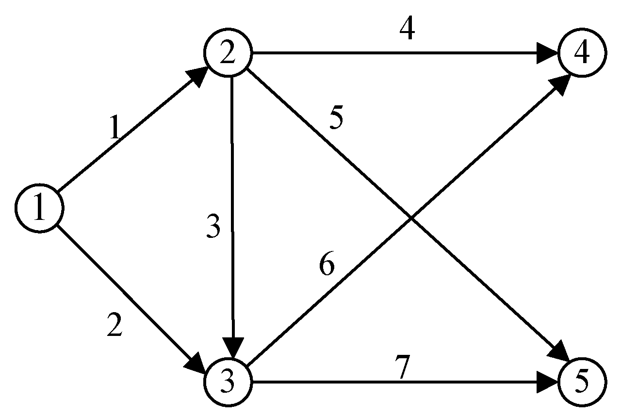
The road network consists of 5 nodes and 7 road sections, node 1 is the origin of the road network, and the destinations are node 4 and node 5. $q_{14}=10$, $q_{15}=15$. The topology of the road network is shown in Figure 2. The road network attributes are shown in

Table 1. Road network attribute table.

Road Section	Free Flow Travel Time (min)	Capacity (pcu/h)	Probability
1	4	25	1
2	5.2	25	0.8
		12.5	0.2
3	1	15	0.9
		7.5	0.1
4	5	15	0.7
		7.5	0.3
5	5	15	1
6	4	15	0.6
		7.5	0.4
7	4	15	1

.

The capacity of road fluctuates with probability. There are 16 road network states in total, which are arranged from large to small according to different state probabilities, as shown in

Table 2. State probability of different road network capacity.

States	${\mathit{P}}_{\mathit{S}}$	States	${\mathit{P}}_{\mathbf{S}}$
(25,25,15,15,15,15,15)	0.3024	(25,25,7.5,15,15,7.5,15)	0.0224
(25,25,15,15,15,7.5,15)	0.2016	(25,12.5,15,7.5,15,7.5,15)	0.0216
(25,25,15,7.5,15,15,15)	0.1296	(25,25,7.5,7.5,15,15,15)	0.0144
(25,25,15,7.5,15,7.5,15)	0.0864	(25,25,7.5,7.5,15,7.5,15)	0.0096
(25,12.5,15,15,15,15,15)	0.0756	(25,12.5,7.5,15,15,15,15)	0.0084
(25,12.5,15,15,15,7.5,15)	0.0504	(25,12.5,7.5,15,15,7.5,15)	0.0056
(25,25,7.5,15,15,15,15)	0.0336	(25,12.5,7.5,7.5,15,15,15)	0.0036
(25,12.5,15,7.5,15,15,15)	0.0324	(25,12.5,7.5,7.5,15,7.5,15)	0.0024

. The BPR (Bureau of Public Road) function is selected as the link impedance function, where let $\alpha =0.15$ and $\beta =4$. In order to simplify the analysis, the threshold value of travel time and travel demand is selected as the same value: $\tau =1.05$, $\mu =1.20$, and the service level correction coefficient is taken as 1. The parameters $\theta =0.05$ which denote traveler’s proficiency in route selection in the SUE model.

4.2. Sensitivity Matrix

After getting a set of equilibrium solutions, the sensitivity matrix can quickly predict the new equilibrium solution after the OD link demand changes. According to the previous model and algorithm design, the reserve capacity can be easily obtained according to the sensitivity matrix.

Taking the capacity state of the first section (25, 25, 15, 15, 15, 15, 15) as an example, the equilibrium solution can be obtained according to MSA, as shown in

Table 3. Equilibrium solution of state 1.

Road Section	Flow(pcu/h)	Road Section	Flow(pcu/h)
1	16.6999	5	5.0267
2	8.3001	6	6.6585
3	8.3316	7	9.9733
4	3.3415

. According to the equilibrium solution of the road section, the Hessian matrix ${\nabla }^{2}L$ can be obtained, and then the sensitivity matrix related to the input flow $q$ can be obtained by calculating the sensitivity equation according to the $\mathit{M}$ and $\mathit{N}$ components.

$$\begin{gathered} {\nabla }^{2}L=\left[\begin{array}{l}0.02862\hspace{0.17em}\hspace{0.17em}\hspace{0.17em}\hspace{0.17em}\hspace{0.17em}\hspace{0.17em}\hspace{0.17em}\hspace{0.17em}\hspace{0.17em}0\hspace{0.17em}\hspace{0.17em}\hspace{0.17em}\hspace{0.17em}\hspace{0.17em}\hspace{0.17em}\hspace{0.17em}\hspace{0.17em}\hspace{0.17em}\hspace{0.17em}\hspace{0.17em}\hspace{0.17em}\hspace{0.17em}\hspace{0.17em}\hspace{0.17em}0\hspace{0.17em}\hspace{0.17em}\hspace{0.17em}\hspace{0.17em}\hspace{0.17em}\hspace{0.17em}\hspace{0.17em}\hspace{0.17em}\hspace{0.17em}\hspace{0.17em}\hspace{0.17em}\hspace{0.17em}\hspace{0.17em}\hspace{0.17em}\hspace{0.17em}0\hspace{0.17em}\hspace{0.17em}\hspace{0.17em}\hspace{0.17em}\hspace{0.17em}\hspace{0.17em}\hspace{0.17em}\hspace{0.17em}\hspace{0.17em}\hspace{0.17em}\hspace{0.17em}\hspace{0.17em}\hspace{0.17em}\hspace{0.17em}\hspace{0.17em}\hspace{0.17em}\hspace{0.17em}0\hspace{0.17em}\hspace{0.17em}\hspace{0.17em}\hspace{0.17em}\hspace{0.17em}\hspace{0.17em}\hspace{0.17em}\hspace{0.17em}\hspace{0.17em}\hspace{0.17em}\hspace{0.17em}\hspace{0.17em}\hspace{0.17em}\hspace{0.17em}0\hspace{0.17em}\hspace{0.17em}\hspace{0.17em}\hspace{0.17em}\hspace{0.17em}\hspace{0.17em}\hspace{0.17em}\hspace{0.17em}\hspace{0.17em}\hspace{0.17em}\hspace{0.17em}\hspace{0.17em}\hspace{0.17em}\hspace{0.17em}\hspace{0.17em}\hspace{0.17em}\hspace{0.17em}\hspace{0.17em}\hspace{0.17em}0\hspace{0.17em}\hspace{0.17em}\hspace{0.17em}\\ \hspace{0.17em}\hspace{0.17em}\hspace{0.17em}\hspace{0.17em}\hspace{0.17em}0\hspace{0.17em}\hspace{0.17em}\hspace{0.17em}\hspace{0.17em}\hspace{0.17em}\hspace{0.17em}\hspace{0.17em}\hspace{0.17em}\hspace{0.17em}1.21165\hspace{0.17em}\hspace{0.17em}\hspace{0.17em}\hspace{0.17em}\hspace{0.17em}-1.20252\hspace{0.17em}\hspace{0.17em}\hspace{0.17em}\hspace{0.17em}\hspace{0.17em}\hspace{0.17em}\hspace{0.17em}\hspace{0.17em}0\hspace{0.17em}\hspace{0.17em}\hspace{0.17em}\hspace{0.17em}\hspace{0.17em}\hspace{0.17em}\hspace{0.17em}\hspace{0.17em}\hspace{0.17em}\hspace{0.17em}\hspace{0.17em}\hspace{0.17em}\hspace{0.17em}\hspace{0.17em}\hspace{0.17em}\hspace{0.17em}\hspace{0.17em}0\hspace{0.17em}\hspace{0.17em}\hspace{0.17em}\hspace{0.17em}\hspace{0.17em}\hspace{0.17em}\hspace{0.17em}\hspace{0.17em}\hspace{0.17em}\hspace{0.17em}\hspace{0.17em}\hspace{0.17em}\hspace{0.17em}\hspace{0.17em}0\hspace{0.17em}\hspace{0.17em}\hspace{0.17em}\hspace{0.17em}\hspace{0.17em}\hspace{0.17em}\hspace{0.17em}\hspace{0.17em}\hspace{0.17em}\hspace{0.17em}\hspace{0.17em}\hspace{0.17em}\hspace{0.17em}\hspace{0.17em}\hspace{0.17em}\hspace{0.17em}\hspace{0.17em}\hspace{0.17em}\hspace{0.17em}0\hspace{0.17em}\hspace{0.17em}\hspace{0.17em}\\ \hspace{0.17em}\hspace{0.17em}\hspace{0.17em}\hspace{0.17em}\hspace{0.17em}0\hspace{0.17em}\hspace{0.17em}\hspace{0.17em}\hspace{0.17em}\hspace{0.17em}\hspace{0.17em}\hspace{0.17em}\hspace{0.17em}\hspace{0.17em}-1.20252\hspace{0.17em}\hspace{0.17em}\hspace{0.17em}1.20483\hspace{0.17em}\hspace{0.17em}\hspace{0.17em}\hspace{0.17em}\hspace{0.17em}\hspace{0.17em}\hspace{0.17em}\hspace{0.17em}\hspace{0.17em}\hspace{0.17em}0\hspace{0.17em}\hspace{0.17em}\hspace{0.17em}\hspace{0.17em}\hspace{0.17em}\hspace{0.17em}\hspace{0.17em}\hspace{0.17em}\hspace{0.17em}\hspace{0.17em}\hspace{0.17em}\hspace{0.17em}\hspace{0.17em}\hspace{0.17em}\hspace{0.17em}\hspace{0.17em}\hspace{0.17em}0\hspace{0.17em}\hspace{0.17em}\hspace{0.17em}\hspace{0.17em}\hspace{0.17em}\hspace{0.17em}\hspace{0.17em}\hspace{0.17em}\hspace{0.17em}\hspace{0.17em}\hspace{0.17em}\hspace{0.17em}\hspace{0.17em}\hspace{0.17em}0\hspace{0.17em}\hspace{0.17em}\hspace{0.17em}\hspace{0.17em}\hspace{0.17em}\hspace{0.17em}\hspace{0.17em}\hspace{0.17em}\hspace{0.17em}\hspace{0.17em}\hspace{0.17em}\hspace{0.17em}\hspace{0.17em}\hspace{0.17em}\hspace{0.17em}\hspace{0.17em}\hspace{0.17em}\hspace{0.17em}\hspace{0.17em}0\hspace{0.17em}\hspace{0.17em}\\ \hspace{0.17em}\hspace{0.17em}\hspace{0.17em}\hspace{0.17em}\hspace{0.17em}0\hspace{0.17em}\hspace{0.17em}\hspace{0.17em}\hspace{0.17em}\hspace{0.17em}\hspace{0.17em}\hspace{0.17em}\hspace{0.17em}\hspace{0.17em}\hspace{0.17em}\hspace{0.17em}\hspace{0.17em}\hspace{0.17em}\hspace{0.17em}0\hspace{0.17em}\hspace{0.17em}\hspace{0.17em}\hspace{0.17em}\hspace{0.17em}\hspace{0.17em}\hspace{0.17em}\hspace{0.17em}\hspace{0.17em}\hspace{0.17em}\hspace{0.17em}\hspace{0.17em}\hspace{0.17em}\hspace{0.17em}0\hspace{0.17em}\hspace{0.17em}\hspace{0.17em}\hspace{0.17em}\hspace{0.17em}\hspace{0.17em}\hspace{0.17em}\hspace{0.17em}\hspace{0.17em}\hspace{0.17em}\hspace{0.17em}\hspace{0.17em}3.98755\hspace{0.17em}\hspace{0.17em}\hspace{0.17em}\hspace{0.17em}\hspace{0.17em}\hspace{0.17em}\hspace{0.17em}\hspace{0.17em}\hspace{0.17em}\hspace{0.17em}\hspace{0.17em}0\hspace{0.17em}\hspace{0.17em}\hspace{0.17em}\hspace{0.17em}\hspace{0.17em}\hspace{0.17em}\hspace{0.17em}\hspace{0.17em}\hspace{0.17em}\hspace{0.17em}\hspace{0.17em}\hspace{0.17em}\hspace{0.17em}\hspace{0.17em}-2\hspace{0.17em}\hspace{0.17em}\hspace{0.17em}\hspace{0.17em}\hspace{0.17em}\hspace{0.17em}\hspace{0.17em}\hspace{0.17em}\hspace{0.17em}\hspace{0.17em}\hspace{0.17em}\hspace{0.17em}\hspace{0.17em}\hspace{0.17em}\hspace{0.17em}\hspace{0.17em}0\\ \hspace{0.17em}\hspace{0.17em}\hspace{0.17em}\hspace{0.17em}\hspace{0.17em}0\hspace{0.17em}\hspace{0.17em}\hspace{0.17em}\hspace{0.17em}\hspace{0.17em}\hspace{0.17em}\hspace{0.17em}\hspace{0.17em}\hspace{0.17em}\hspace{0.17em}\hspace{0.17em}\hspace{0.17em}\hspace{0.17em}\hspace{0.17em}0\hspace{0.17em}\hspace{0.17em}\hspace{0.17em}\hspace{0.17em}\hspace{0.17em}\hspace{0.17em}\hspace{0.17em}\hspace{0.17em}\hspace{0.17em}\hspace{0.17em}\hspace{0.17em}\hspace{0.17em}\hspace{0.17em}\hspace{0.17em}0\hspace{0.17em}\hspace{0.17em}\hspace{0.17em}\hspace{0.17em}\hspace{0.17em}\hspace{0.17em}\hspace{0.17em}\hspace{0.17em}\hspace{0.17em}\hspace{0.17em}\hspace{0.17em}\hspace{0.17em}\hspace{0.17em}\hspace{0.17em}\hspace{0.17em}\hspace{0.17em}0\hspace{0.17em}\hspace{0.17em}\hspace{0.17em}\hspace{0.17em}\hspace{0.17em}\hspace{0.17em}\hspace{0.17em}\hspace{0.17em}\hspace{0.17em}\hspace{0.17em}\hspace{0.17em}\hspace{0.17em}\hspace{0.17em}2.65285\hspace{0.17em}\hspace{0.17em}\hspace{0.17em}\hspace{0.17em}\hspace{0.17em}\hspace{0.17em}\hspace{0.17em}\hspace{0.17em}0\hspace{0.17em}\hspace{0.17em}\hspace{0.17em}\hspace{0.17em}\hspace{0.17em}\hspace{0.17em}\hspace{0.17em}\hspace{0.17em}\hspace{0.17em}\hspace{0.17em}\hspace{0.17em}-1.33333\\ \hspace{0.17em}\hspace{0.17em}\hspace{0.17em}\hspace{0.17em}\hspace{0.17em}0\hspace{0.17em}\hspace{0.17em}\hspace{0.17em}\hspace{0.17em}\hspace{0.17em}\hspace{0.17em}\hspace{0.17em}\hspace{0.17em}\hspace{0.17em}\hspace{0.17em}\hspace{0.17em}\hspace{0.17em}\hspace{0.17em}\hspace{0.17em}0\hspace{0.17em}\hspace{0.17em}\hspace{0.17em}\hspace{0.17em}\hspace{0.17em}\hspace{0.17em}\hspace{0.17em}\hspace{0.17em}\hspace{0.17em}\hspace{0.17em}\hspace{0.17em}\hspace{0.17em}\hspace{0.17em}\hspace{0.17em}0\hspace{0.17em}\hspace{0.17em}\hspace{0.17em}\hspace{0.17em}\hspace{0.17em}\hspace{0.17em}\hspace{0.17em}\hspace{0.17em}\hspace{0.17em}\hspace{0.17em}\hspace{0.17em}\hspace{0.17em}\hspace{0.17em}\hspace{0.17em}-2\hspace{0.17em}\hspace{0.17em}\hspace{0.17em}\hspace{0.17em}\hspace{0.17em}\hspace{0.17em}\hspace{0.17em}\hspace{0.17em}\hspace{0.17em}\hspace{0.17em}\hspace{0.17em}\hspace{0.17em}\hspace{0.17em}\hspace{0.17em}\hspace{0.17em}\hspace{0.17em}0\hspace{0.17em}\hspace{0.17em}\hspace{0.17em}\hspace{0.17em}\hspace{0.17em}\hspace{0.17em}\hspace{0.17em}\hspace{0.17em}\hspace{0.17em}\hspace{0.17em}\hspace{0.17em}1.10764\hspace{0.17em}\hspace{0.17em}\hspace{0.17em}\hspace{0.17em}\hspace{0.17em}\hspace{0.17em}\hspace{0.17em}\hspace{0.17em}\hspace{0.17em}\hspace{0.17em}\hspace{0.17em}\hspace{0.17em}0\hspace{0.17em}\hspace{0.17em}\hspace{0.17em}\hspace{0.17em}\hspace{0.17em}\hspace{0.17em}\\ \hspace{0.17em}\hspace{0.17em}\hspace{0.17em}\hspace{0.17em}\hspace{0.17em}0\hspace{0.17em}\hspace{0.17em}\hspace{0.17em}\hspace{0.17em}\hspace{0.17em}\hspace{0.17em}\hspace{0.17em}\hspace{0.17em}\hspace{0.17em}\hspace{0.17em}\hspace{0.17em}\hspace{0.17em}\hspace{0.17em}\hspace{0.17em}0\hspace{0.17em}\hspace{0.17em}\hspace{0.17em}\hspace{0.17em}\hspace{0.17em}\hspace{0.17em}\hspace{0.17em}\hspace{0.17em}\hspace{0.17em}\hspace{0.17em}\hspace{0.17em}\hspace{0.17em}\hspace{0.17em}\hspace{0.17em}0\hspace{0.17em}\hspace{0.17em}\hspace{0.17em}\hspace{0.17em}\hspace{0.17em}\hspace{0.17em}\hspace{0.17em}\hspace{0.17em}\hspace{0.17em}\hspace{0.17em}\hspace{0.17em}\hspace{0.17em}\hspace{0.17em}\hspace{0.17em}\hspace{0.17em}\hspace{0.17em}0\hspace{0.17em}\hspace{0.17em}\hspace{0.17em}\hspace{0.17em}\hspace{0.17em}\hspace{0.17em}\hspace{0.17em}\hspace{0.17em}\hspace{0.17em}\hspace{0.17em}\hspace{0.17em}\hspace{0.17em}-1.33333\hspace{0.17em}\hspace{0.17em}\hspace{0.17em}\hspace{0.17em}\hspace{0.17em}\hspace{0.17em}\hspace{0.17em}0\hspace{0.17em}\hspace{0.17em}\hspace{0.17em}\hspace{0.17em}\hspace{0.17em}\hspace{0.17em}\hspace{0.17em}\hspace{0.17em}\hspace{0.17em}\hspace{0.17em}\hspace{0.17em}\hspace{0.17em}\hspace{0.17em}0.71905\hspace{0.17em}\hspace{0.17em}\hspace{0.17em}\hspace{0.17em}\end{array}\right] \\ \begin{array}{l}\left[\frac{\partial x_{12}}{\partial {\gamma }_{14}},\frac{\partial x_{13}}{\partial {\gamma }_{14}},\frac{\partial x_{23}}{\partial {\gamma }_{14}},\frac{\partial x_{24}}{\partial {\gamma }_{14}},\frac{\partial x_{25}}{\partial {\gamma }_{14}},\frac{\partial x_{34}}{\partial {\gamma }_{14}},\frac{\partial x_{35}}{\partial {\gamma }_{14}}\right]=\left[0.6630,0.3370,0.3300,0.3343,-0.0013,0.6657,0.0013\right]\\ \left[\frac{\partial x_{12}}{\partial {\gamma }_{15}},\frac{\partial x_{13}}{\partial {\gamma }_{15}},\frac{\partial x_{23}}{\partial {\gamma }_{15}},\frac{\partial x_{24}}{\partial {\gamma }_{15}},\frac{\partial x_{25}}{\partial {\gamma }_{15}},\frac{\partial x_{34}}{\partial {\gamma }_{15}},\frac{\partial x_{35}}{\partial {\gamma }_{15}}\right]=\left[\hspace{0.17em}0.6654,0.3346,0.3276,-0.0008,0.3386,0.0008,0.6614\right]\end{array} \end{gathered}$$

At state 7, the equilibrium solution is shown in

Table 4. Equilibrium solution of state 7.

Road Section	Flow(pcu/h)	Road Section	Flow(pcu/h)
1	16.2867	5	5.2772
2	8.7133	6	6.4905
3	7.5000	7	9.7228
4	3.5095

, and the road Section 3 reaches the capacity limit, the sensitivity matrix between the link flow and the OD demand can be obtained.

$$\begin{array}{l}\left[\frac{\partial x_{12}}{\partial {\gamma }_{14}},\frac{\partial x_{13}}{\partial {\gamma }_{14}},\frac{\partial x_{23}}{\partial {\gamma }_{14}},\frac{\partial x_{24}}{\partial {\gamma }_{14}},\frac{\partial x_{25}}{\partial {\gamma }_{14}},\frac{\partial x_{34}}{\partial {\gamma }_{14}},\frac{\partial x_{35}}{\partial {\gamma }_{14}}\right]=\left[0.4993,0.5007,0.0000,0.4110,-0.0883,0.5890,0.0883\right]\\ \left[\frac{\partial x_{12}}{\partial {\gamma }_{15}},\frac{\partial x_{13}}{\partial {\gamma }_{15}},\frac{\partial x_{23}}{\partial {\gamma }_{15}},\frac{\partial x_{24}}{\partial {\gamma }_{15}},\frac{\partial x_{25}}{\partial {\gamma }_{15}},\frac{\partial x_{34}}{\partial {\gamma }_{15}},\frac{\partial x_{35}}{\partial {\gamma }_{15}}\right]=\left[\hspace{0.17em}0.5026,0.4974,0.0000,0.0588,0.4438,-0.0588,0.5562\right]\end{array}$$

It can be found that according to the sensitivity matrix, when OD demand increases, the traffic flow of Section 3 will not increase. In the analysis of reserve capacity, it can be considered that the increase of traffic demand will not bring about the increase of saturation of this section, and this section can be eliminated in the analysis.

4.3. Reliability Analysis

According to the sensitivity matrix, the upper-level model of the bi-level model for reliability analysis can be transformed into a simple linear programming problem.

Taking the capacity state of the first road section (25, 25, 15, 15, 15, 15, 15), the reserve capacity coefficient under capacity constraint is ${\mu }_{\gamma c}=1.5067$, the reserve capacity coefficient under travel time constraint is ${\mu }_{\gamma t}=1.6866$, and the minimum value is taken as the initial reserve capacity coefficient ${\mu }_{\gamma }{}^{(n)}=1.5067$.

According to step 3 (see the algorithm design part for details), we can get ${\mu }_{\gamma }{}^{(n+1)}=1.0062$, the convergence condition is $\left|{\mu }_{\gamma }{}^{(n+1)}{\mu }_{\gamma }{}^{(n)}-{\mu }_{\gamma }{}^{(n)}\right|=0.0094\le 0.01$, then getting the reserve capacity coefficient ${\mu }_{\gamma }=1.5067\ast 1.0062=1.5160$.

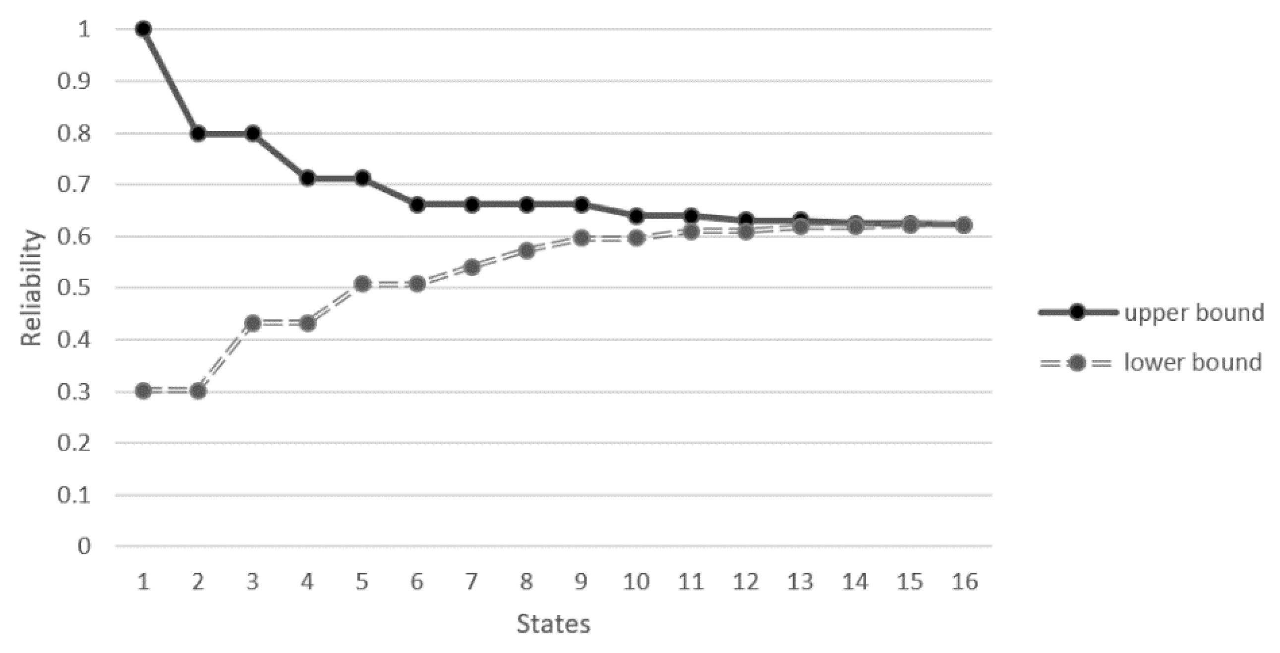
Similarly, the reserve capacity under other conditions can be obtained, as shown in

Table 5. List of reserve capacity in capacity status of each road section.

States	${\mathit{\mu }}_{\mathit{\gamma }}$	States	${\mathit{\mu }}_{\mathit{\gamma }}$
(25,25,15,15,15,15,15)	1.5160	(25,25,7.5,15,15,7.5,15)	1.6319
(25,25,15,15,15,7.5,15)	1.1247	(25,12.5,15,7.5,15,7.5,15)	1.1350
(25,25,15,7.5,15,15,15)	1.5077	(25,25,7.5,7.5,15,15,15)	1.6326
(25,25,15,7.5,15,7.5,15)	1.1243	(25,25,7.5,7.5,15,7.5,15)	1.1480
(25,12.5,15,15,15,15,15)	1.5084	(25,12.5,7.5,15,15,15,15)	1.5145
(25,12.5,15,15,15,7.5,15)	1.1250	(25,12.5,7.5,15,15,7.5,15)	1.1480
(25,25,7.5,15,15,15,15)	1.6325	(25,12.5,7.5,7.5,15,15,15)	1.5142
(25,12.5,15,7.5,15,15,15)	1.5084	(25,12.5,7.5,7.5,15,7.5,15)	1.1491

. Then, through the approximation form of upper bound and lower bound function, the reliability of the example road network is 0.6224, as shown in

Table 6. Reliability upper and lower bounds analysis based on road network capacity.

States	${\mathit{P}}_{\mathit{S}}$		States	${\mathit{P}}_{\mathit{S}}$
	Upper Bound	Lower Bound		Upper Bound	Lower Bound
(25,25,15,15,15,15,15)	1	0.3024	(25,25,7.5,15,15,7.5,15)	0.6616	0.596
(25,25,15,15,15,7.5,15)	0.7984	0.3024	(25,12.5,15,7.5,15,7.5,15)	0.64	0.596
(25,25,15,7.5,15,15,15)	0.7984	0.432	(25,25,7.5,7.5,15,15,15)	0.64	0.6104
(25,25,15,7.5,15,7.5,15)	0.712	0.432	(25,25,7.5,7.5,15,7.5,15)	0.6304	0.6104
(25,12.5,15,15,15,15,15)	0.712	0.5076	(25,12.5,7.5,15,15,15,15)	0.6304	0.6188
(25,12.5,15,15,15,7.5,15)	0.6616	0.5076	(25,12.5,7.5,15,15,7.5,15)	0.6248	0.6188
(25,25,7.5,15,15,15,15)	0.6616	0.5412	(25,12.5,7.5,7.5,15,15,15)	0.6248	0.6224
(25,12.5,15,7.5,15,15,15)	0.6616	0.5736	(25,12.5,7.5,7.5,15,7.5,15)	0.6224	0.6224

and Figure 3.

In order to improve the reliability, the capacity of all road sections is increased by 10%. It can be found that the range of reliability improvement is different, as shown in

Table 7. Analysis table of contribution degree of road network reliability improvement.

Road Section	Capacity	Capacity Increased by 10%	Reliability	Reliability Improvement Range
1	25	27.5	0.6224	0.00%
2	25	27.5	0.6224	0.00%
	12.5	13.75
3	15	16.5	0.6332	1.74%
	7.5	8.25
4	15	16.5	0.6344	1.93%
	7.5	8.25
5	15	16.5	0.6224	0.00%
6	15	16.5	0.9944	59.77%
	7.5	8.25
7	15	16.5	0.6224	0.00%

. The contribution of road is the largest. The improvement of some road sections has no contribution to the improvement of road network reliability. Therefore, to improve the reliability of the road network, it is necessary to upgrade the key sections.

4.4. Reliability Analysis by Traditional Method

Equation (4) is the traditional model to obtain the reserve capacity, its lower-level model has no capacity constraints, so at the state of low road capacity, the distribution flow may exceed the capacity of the road section, the reserve capacity is 1.

Taking state of 7 as an example, in the case of no capacity constraint, if the results are not optimized by the Lagrange multiplier method, the results are shown in

Table 8. Equilibrium solution of state 7 without optimized.

Road Section	Flow(pcu/h)	Road Section	Flow(pcu/h)
1	16.6713	5	5.0440
2	8.3287	6	6.6469
3	8.2742	7	9.9560
4	3.3531

. At this time, the flow of the road Section 3 is greater than the capacity: $x_{23}=8.2742>7.5$, so we get the ${\mu }_r{}^{n+1}<1$ by upper-level model, so the reserve capacity is ${\mu }_r=\max ({\mu }_r{}^{n+1}{\mu }_r{}^n,{\mu }_r{}^n)=1$. But in the actual situation, the distribution flow will not be higher than the link capacity, so this analysis result has some problems.

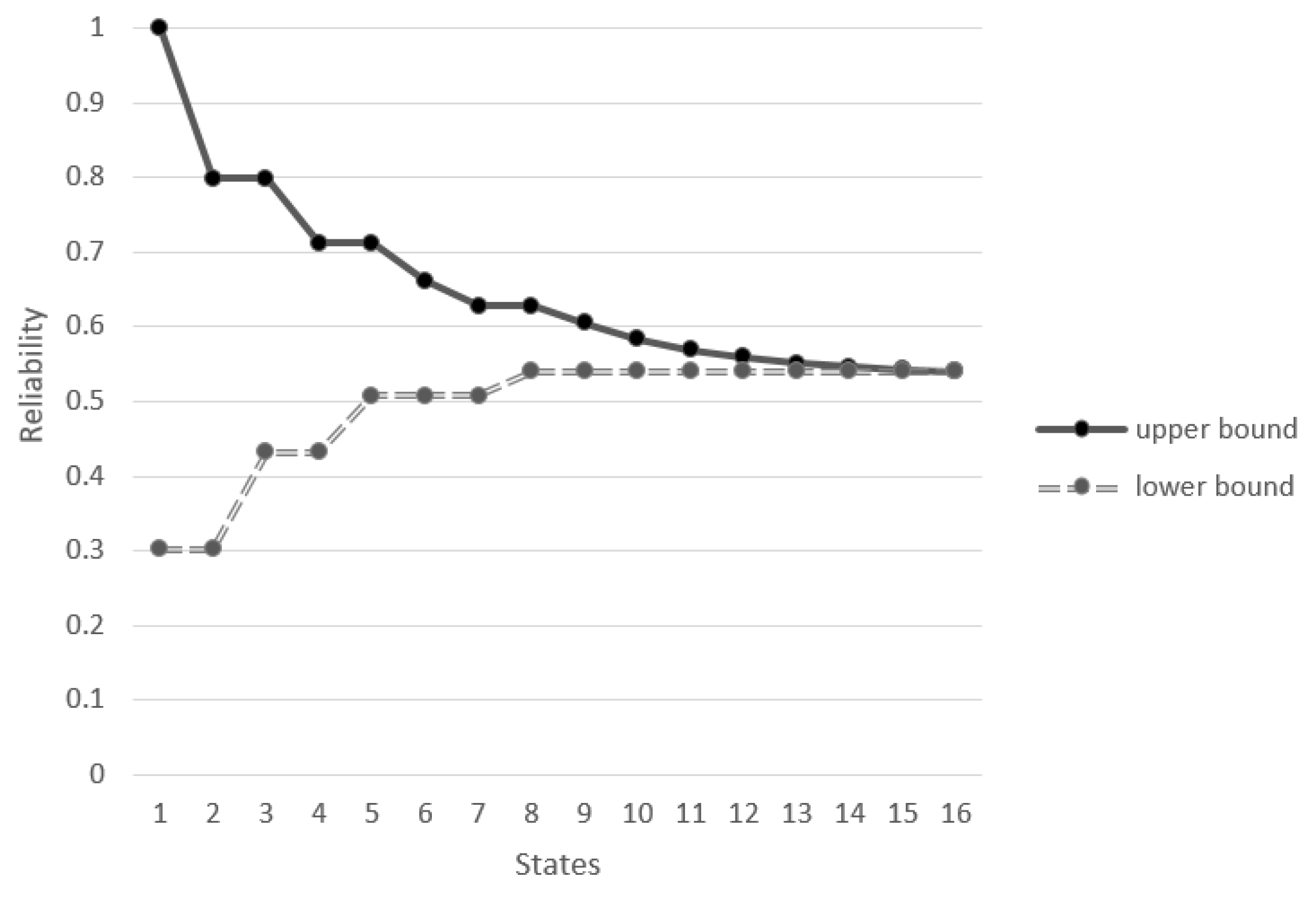
The traditional upper-level model is simple, there is no limit to the acceptability of the link formation time, so the result will be different from that of the improved model, such as the state of 2, it is shown in

Table 9. List of reserve capacity in capacity status of each road section.

States	${\mathit{\mu }}_{\mathit{\gamma }}$	States	${\mathit{\mu }}_{\mathit{\gamma }}$
(25,25,15,15,15,15,15)	1.5067	(25,25,7.5,15,15,7.5,15)	1
(25,25,15,15,15,7.5,15)	1.1330	(25,12.5,15,7.5,15,7.5,15)	1.1335
(25,25,15,7.5,15,15,15)	1.5077	(25,25,7.5,7.5,15,15,15)	1
(25,25,15,7.5,15,7.5,15)	1.1323	(25,25,7.5,7.5,15,7.5,15)	1
(25,12.5,15,15,15,15,15)	1.5084	(25,12.5,7.5,15,15,15,15)	1
(25,12.5,15,15,15,7.5,15)	1.1342	(25,12.5,7.5,15,15,7.5,15)	1
(25,25,7.5,15,15,15,15)	1	(25,12.5,7.5,7.5,15,15,15)	1
(25,12.5,15,7.5,15,15,15)	1.5084	(25,12.5,7.5,7.5,15,7.5,15)	1

. Then, through the approximation form of upper bound and lower bound function, the reliability of the example road network is 0.54, as shown in

Table 10. Reliability upper and lower bounds analysis based on road network capacity.

States	Ps		States	Ps
	Upper Bound	Lower Bound		Upper Bound	Lower Bound
(25,25,15,15,15,15,15)	1	0.3024	(25,25,7.5,15,15,7.5,15)	0.6056	0.54
(25,25,15,15,15,7.5,15)	0.7984	0.3024	(25,12.5,15,7.5,15,7.5,15)	0.584	0.54
(25,25,15,7.5,15,15,15)	0.7984	0.432	(25,25,7.5,7.5,15,15,15)	0.5696	0.54
(25,25,15,7.5,15,7.5,15)	0.712	0.432	(25,25,7.5,7.5,15,7.5,15)	0.56	0.54
(25,12.5,15,15,15,15,15)	0.712	0.5076	(25,12.5,7.5,15,15,15,15)	0.5516	0.54
(25,12.5,15,15,15,7.5,15)	0.6616	0.5076	(25,12.5,7.5,15,15,7.5,15)	0.546	0.54
(25,25,7.5,15,15,15,15)	0.628	0.5076	(25,12.5,7.5,7.5,15,15,15)	0.5424	0.54
(25,12.5,15,7.5,15,15,15)	0.628	0.54	(25,12.5,7.5,7.5,15,7.5,15)	0.54	0.54

and Figure 4. The reliability of the road network is far lower than that result of the improved model.

Because the results of traffic flow assignment of traditional model do not conform to the law of reality, and the travel time acceptability is not considered, so the improved model allocation results are more reliable.

5. Discussion

According to the results of the previous analysis, improving the reliability of the road network can start from two aspects: traffic demand control and road section improvement. Under the condition that traffic demand does not increase or the growth is very small (less than the reserve capacity), if the current traffic operation is relatively good, the overall reliability of the road network is “1”. The common traffic demand management means including traffic restriction in peak hours, rush hour commuting, etc. In the aspect of road section improvement, more attention should be paid to the key sections. Based on the contribution of road sections to reliability, the article identifies key sections, and the improvement methods include road widening, section reconstruction, etc. However, in the face of the large-scale road network, it is difficult to identify the key road sections by contribution degree, so the comprehensive judgment method can be adopted: take the intersection of the congested section and sensitive section [31].

This article improves the reliability analysis model and algorithm, and applies it to a small example, and puts forward the direction of improving the reliability of the road network. In the future, it can be applied to the actual large-scale road network, which can reflect the improvement efficiency of the algorithm. At the same time, the analysis results can provide certain reference for urban management.

References

- Mine, H.; Kawai, H. Mathematics for Reliability Analysis; Asakura Shoten: Tokyo, Japan, 1982. [Google Scholar]
- Iida, Y.; Wakabayashi, H. An Approximation Method of Terminal Reliability of Road Network Using Partial Minimal Path and Cut Sets. In Proceedings of the Transport Policy, Management & Technology towards 2001: Selected Proceedings of the Fifth World Conference on Transport Research, Yokohama, Japan, 10–14 July 1989. [Google Scholar]
- Nicholson, A.; Schmöcker, J.-D.; Bell, M.G.H.; Iida, Y. Assessing Transport Reliability: Malevolence and User Knowledge. In The Network Reliability of Transport; Emerald Publishers: Chennai, India, 2003; pp. 1–22. [Google Scholar]
- Bell, M.G.H.; Lida, Y. Transportation Network Analysis; John Wiley & Sons, Inc.: Hoboken, NJ, USA, 1997. [Google Scholar]
- Liao, Y.-Q.; Jia, L.-M.; Li, S.; Li, C.-X.; Dong, H.-H. Research on the Connectivity Reliability of Transport Networks. J. Transp. Eng. Inf. 2011, 9, 30–34. [Google Scholar]
- Li, B.; Hu, X.; Xie, B. Transportation Network Reconstruction for Natural Disasters in Emergency Phase Based on Connectivity Reliability. In Proceedings of the Second International Conference on Transportation Engineering, Chengdu, China, 25–27 July 2009; pp. 108–112. [Google Scholar]
- Asakura, Y. Reliability Measures of an Origin and Destination Pair in a Deteriorated Road Network with Variable Flows. Transp. Netw. Recent Methodol. Adv. 1999, 1999, 273–287. [Google Scholar] [CrossRef]
- Iida, Y. Basic concepts and future directions of road network reliability analysis. J. Adv. Transp. 1999, 33, 125–134. [Google Scholar] [CrossRef]
- Al-Deek, H.; Emam, E.B. New Methodology for Estimating Reliability in Transportation Networks with Degraded Link Capacities. J. Intell. Transp. Syst. 2006, 10, 117–129. [Google Scholar] [CrossRef]
- Lo, K.K.; Yang, H.; Tang, W.H. Combining Travel Time and Capacity Reliability for Performance Measure of a Road Network. J. Am. Diet. Assoc. 1999, 109 (Suppl. S9), A66. [Google Scholar]
- Clark, S.; Watling, D. Modeling network travel time reliability under stochastic demand. Transp. Res. Part B 2005, 39, 119–140. [Google Scholar]
- Mahmassani, H.S.; Hou, T.; Saberi, M. Connecting Networkwide Travel Time Reliability and the Network Fundamental Diagram of Traffic Flow. Transp. Res. Rec. J. Transp. Res. Board 2013, 2391, 80–91. [Google Scholar]
- Zhang, X.; Li, R.; Li, H. Study on Travel Time Reliability Based on Monte Carlo Method. J. Wuhan Univ. Technol. 2012, 36, 667–670. [Google Scholar]
- Aggarwal, K.K. Integration of Reliability and Capacity in Performance Measure of a Telecommunication Network. IEEE Trans. Reliab. 2009, R-34, 184–186. [Google Scholar]
- Chan, Y.; Yim, E.; Marsh, A. Exact and approximate improvement to the throughput of a stochastic network. IEEE Trans. Reliab. 1997, 46, 473–486. [Google Scholar] [CrossRef]
- Billinton, R.; Li, W. Reliability Assessment of Electric Power Systems Using Monte Carlo Methods. Reliab. Assess. Electr. Power Syst. Using Monte Carlo Methods 1994, 1994, 9–31. [Google Scholar] [CrossRef]
- Li, D.; Doležal, T.; Haimes, Y.Y. Capacity reliability of water distribution networks. Reliab. Eng. Syst. Saf. 1993, 42, 29–38. [Google Scholar] [CrossRef]
- Chen, A.; Yang, H.; Lo, H.K.; Tang, W.H. Capacity reliability of a road network: An assessment methodology and numerical results. Transp. Res. Part B Methodol. 2002, 36, 225–252. [Google Scholar] [CrossRef]
- Chen, A.; Yang, H.; Lo, H.K.; Tang, W.H. A capacity related reliability for transportation networks. J. Adv. Transp. 1999, 33, 183–200. [Google Scholar] [CrossRef]
- Bell, M.G.H.; Schmöcker, J.D. Network Reliability: Topological Effects and the Importance of Information. In Proceedings of the International Conference on Traffic and Transportation Studies, Guilin, China, 23–25 July 2002; pp. 453–460. [Google Scholar]
- Wong, K.I.; Bell, M.G.H. An evaluation of reliability of taxi service quality. In Proceedings of the 2nd International Symposium on Transportation Network Reliability, Queenstown, New Zeland, 20–24 August 2004; pp. 8–14. [Google Scholar]
- Lo, H.K. A reliability framework for traffic signal control. IEEE Trans. Intell. Transp. Syst. 2006, 7, 250–260. [Google Scholar]
- Vaessen, J. Accessibility of Rural Credit in Northern Nicaragua: The Importance of Networks of Information and Recommen-Dation. Work. Pap. 2007, 25, 5–32. [Google Scholar]
- Bingxun, T. Traffic congestion and road service level. Road Traffic Saf. 2004, 4, 10–14. [Google Scholar]
- Fisk, C. Some developments in equilibrium traffic assignment methodology. Transp. Res. 1980, 14, 243–256. [Google Scholar] [CrossRef]
- Akamatsu, T. Decomposition of Path Choice Entropy in General Transport Networks. Transp. Sci. 1997, 31, 349–362. [Google Scholar] [CrossRef]
- Ji, K.; Cheng, L.; Tang, W. Model and Algorithm for Link-Based Stochastic User Equilibrium Traffic Assignment. In Proceedings of the Twelfth COTA International Conference of Transportation Professionals, Beijing, China, 3–6 August 2012; pp. 579–591. [Google Scholar]
- Lee, D.-H.; Meng, Q.; Deng, W. Origin-Based partial linearization method for stochastic user equilibrium traffic assignment problem. J. Transp. Eng. 2010, 136, 52–60. [Google Scholar]
- Ji, K.; Ma, J.; Tang, W. Sensitivity analysis for stochastic user equilibrium traffic assignment with constraints. Adv. Mech. Eng. 2017, 9. [Google Scholar] [CrossRef] [Green Version]
- Chen, L.; Ji, K.; Pu, Z.; Wang, Y. Sensitivity analysis for link-based stochastic user Chen equilibrium network flows. J. Southeast Univ. 2013, 43, 221–225. [Google Scholar]
- Gao, A. A Study on the Urban Road Network Reliability and Its Safeguards Technology. Ph.D. Thesis, Beijing University of Technology, Beijing, China, 2010. [Google Scholar]
Figure 1.
Flowchart of the algorithm.
Figure 2.
Example road network diagram.
Figure 3.
Reliability upper and lower bounds analysis based on road network capacity.
Figure 4.