Variation Trends of Fractal Dimension in Epileptic EEG Signals

Abstract

Epileptic diseases take EEG as an important basis for clinical judgment, and fractal algorithms were often used to analyze electroencephalography (EEG) signals. However, the variation trends of fractal dimension (D) were opposite in the literature, i.e., both D decreasing and increasing were reported in previous studies during seizure status relative to the normal status, undermining the feasibility of fractal algorithms for EEG analysis to detect epileptic seizures. In this study, two algorithms with high accuracy in the D calculation, Higuchi and roughness scaling extraction (RSE), were used to study D variation of EEG signals with seizures. It was found that the denoising operation had an important influence on D variation trend. Moreover, the D variation obtained by RSE algorithm was larger than that by Higuchi algorithm, because the non-fractal nature of EEG signals during normal status could be detected and quantified by RSE algorithm. The above findings in this study could be promising to make more understandings of the nonlinear nature and scaling behaviors of EEG signals.

1. Introduction

Electroencephalography (EEG) signals have been widely used in various fields [1,2,3,4,5] in recent years because it is easy to measure and could be displayed in real time. It is very important to analyze EEG and obtain its implicit correct and important information, because that EEG signals is closely related to brain activity, which could reflect the psychological state, emotional changes, brain activity and the body functionalities, etc. [6]. Therefore, EEG is crucial for understanding the information processing of the human brain [4], enabling the investigations on human brain activity and cognitive processes. The study of effective changes through EEG signals also could promote learning and works [1]. At the same time, EEG signals could also be used to detect psychological and physiological diseases [5,7], which played an important role in the advanced knowledge and treatment of major depression [2,3], autism [1], schizophrenia [8], Parkinson’s syndrome [9] and epilepsy. In addition, EEG signals can be used to measure emotion recognition [10,11,12] and sleep quality [13], and had important applications in neuromarketing [14], biometrics [15] and brain–computer interface and games [16].

In the recent decades, EEG signals have been one of the most important approaches in clinical disease diagnosis and have authoritative diagnostic information for epilepsy [17]. Epilepsy is a common mental disease, which is a chronic mental disease caused by the sudden and temporary disorder of brain function, which could attributed to the paroxysmal abnormal discharge of brain nerve cells. The detection of epilepsy mainly refers to EEG signals, according to the clinical manifestations and EEG signals records of patients to judge epileptic seizures, and according to the EEG signals for epileptic seizure lesion location, efficacy and postoperative evaluation. Therefore, it is quite necessary to study the algorithms that could accurately analyze EEG signals for the automatic detection of epileptic seizures. Using the fractal algorithm to detect epileptic seizures was an important method and had been demonstrated [18,19]. Currently, there were many commonly used fractal algorithms, among which the Higuchi algorithm was highly recommended because of its accuracy and high speed [20,21]. In our previous studies, roughness scaling extraction (RSE) algorithm was proposed to detect epileptic seizures, which could be more accurate to calculate fractal dimension (D) relative to the traditional algorithms including Higuchi algorithm [22,23].

An important basis for using the fractal algorithms to detect epileptic seizures was the D variation during seizure status compared with normal status. However, it was found that some publications reported that D in the seizure status had a downward trend [21,24,25], while other literature reported an upward trend of D variation [20,22,23,26,27], and such a significant divergence and its cause had not been studied in the available literature. Such a significant difference seriously undermined the feasibility and even the reliability of fractal algorithms in epileptic detection. Therefore, it would be of great importance to carry out an investigation on which trend of D variation in the seizure status should own and the underlying mechanism of the divergence mentioned above.

In this study, based on EEG signals of the CHB-MIT Scalp EEG Database, both Higuchi and RSE algorithms with high accuracy in D calculation were used to calculate D values of epileptic EEG signals and study the D variation during seizure status compared with normal status. The denoising process for EEG signals was essential and there were lots of noise reduction methods, such as wavelet decomposition [28,29] and empirical mode decomposition (EMD) [30,31]. To be consistent with previous research, the denoising process in this study was wavelet decomposition with passband filtering and had been widely used to alleviate the noise influences [22,23,28,29]. The reason for the above-mentioned difference of D variations were analyzed and it was found that the denoising operation had an important influence on D variation trend. Besides, the effects of signal denoising and algorithm accuracy in the detection of epileptic seizures were discussed based on the statistical analysis on the caculated results.

2. Data and Methods

2.1. EEG Signals

The EEG signals used in this study were from the CHB-MIT Scalp EEG Database [32,33,34], which was collected at the Children’s Hospital Boston, consisting of EEG recordings from pediatric subjects with intractable seizures. All the EEG signals were sampled at 256 Hz. There were 198 recordings of seizures in the CHB-MIT database, 109 effective recordings of seizures were selected based on the time length (800 s) and seizure recognition for comparison.

Table 1. EEG signals used in this study from CHB-MIT Scalp EEG Database.

File Names (Patients)	Seizure Labels	Number	Seizure Durations (s)
CHB01 (1)	6	1–6	400–(440,427,440,451,490,501)
CHB03 (3)	6	7–12	400–(465,469,452,447,464,453)
CHB04 (4)	3	13–15	400–(511,505,516)
CHB05 (5)	5	16–20	400–(515,510,496,520,517)
CHB06 (6)	8	21–28	400–(414,415,415,420,416,412,413,416)
CHB07 (7)	2	29–30	400–(486,496)
CHB09 (9)	4	31–34	400–(464,479,471,462)
CHB10 (10)	2	35–36	400–(489,454)
CHB12 (12)	31	37–67	400–(461,413,423,420,432,432, 445,437,497,440,435,427, 425,442,452,448,438,436, 446,421,423,427,425,423, 443,455,451,428,429,425,423)
CHB13 (13)	1	68	400–465
CHB14 (14)	7	69–75	400–(414,420,422,414,441,422,416)
CHB15 (15)	1	76	400–577
CHB16 (16)	1	77	400–414
CHB17 (17)	3	78–80	400–(490,515,488)
CHB18 (18)	3	81–83	400–(455,468,446)
CHB19 (19)	1	84	400–477
CHB20 (20)	6	85–90	400–(430,439,438,449,435,439)
CHB21 (21)	1	91	400–412
CHB22 (22)	2	92–93	400–(474,472)
CHB23 (23)	6	94–99	400–(513,447,471,462,427,484)
CHB24 (24)	10	100–109	400–(425,425,425,432,427,419, 424,419,427,468)

contained the descriptions for each recording obtained by the CHB-MIT database and included the file names of the EEG signals, labels of seizure, number of calculation and seizure durations.

2.2. Higuchi Algorithm

Higuchi algorithm [35] is based on the length measurement of signals $L\left(k\right)$. Taking k sampling points as the unit, D satisfies:

$$L\left(k\right)\propto k^{-D}$$

(1)

For signal $X=x\left(1\right),x\left(2\right),x\left(3\right),\dots ,x\left(N\right)$, $k=k_{min},\dots ,k_{max}$, rebuild k new time series: $X_k^m=x\left(m\right),x(m+k),x(m+2k),\dots ,x(m+\lfloor \frac{N-m}{k}\rfloor ·k)$, $m=1,2,3,\dots ,k$, among them: m is the initial point, k is the interval, $\lfloor \rfloor$ denotes the Gauss’ notation and both m and k are integers. For k reconstructed new sequences, calculate the length of each sequence $L_m\left(k\right)$:

$$L_m\left(k\right)=\frac{1}{k}·\left(\sum _{i=1}^{\lfloor (N-m)/k\rfloor }\mid x(m+i·k)-x[m+(i-1)·k]\mid \right)·\frac{N-1}{\lfloor (N-m)/k\rfloor ·k}$$

(2)

N is the total number of signal, and $\frac{N-1}{\lfloor (N-m)/k\rfloor ·k}$ is the normalization correction factor. Take the average length of k sequences with the same interval as the signal length $L\left(k\right)$ corresponding to interval k, namely:

$$L\left(k\right)=\frac{1}{k}\sum _{m=1}^k{L}_m\left(k\right)$$

(3)

$$lnL\left(k\right)\propto -Dlnk$$

(4)

Given that each signal series $X\left(k\right)$ and the corresponding series length $L\left(k\right)$, fitted in the double logarithmic coordinates, D is the opposite slope of the signal. The accuracy of Higuchi algorithm is generally high under various noise levels when $k_{max}$ is in 40 and 50 based on the previous literature [36,37], and $k_{max}=42$ is used in this study.

2.3. RSE Algorithm

RSE algorithm is based on the scaling relationship of root-mean-squared roughness ($Rq$) and the data-point length (L), which satisfy:

$$Rq=A{L}^H=A{L}^{2-D}$$

(5)

Among this equation, A: $Rq$ value when $L=1$; H: Hurst exponent ($0<H<1$); D: fractal dimension ($D=2-H$). The $Rq$ and L of the fractal curve satisfy the above equation, and D can be obtained by fitting a straight line to them in the double logarithmic coordinate system:

$$lnRq=(2-D)lnL+lnA$$

(6)

The special feature of RSE algorithm was the flattening operation on the segmented sub-series in prior to $Rq$ calculation, whose details could be found in our previous publication [22]. Therefore, the RSE algorithms with various flattening orders were denoted in this study as RSE-f1 and RSE-f2, which used first-order polynomials ($y_{f1}=ax+b$) and second-order polynomials ($y_{f2}=a{x}^2+bx+c$), respectively.

However, the $Rq-L$ curves in double logarithmic coordinates obtained in RES algorithms was not linear globally. In our recent work [38], it has been demonstrated that such a linear scope, named as scaling region, was the efficient partial for D calculation, and a scaling region interception method was proposed to enhance the accuracy of RSE algorithm.

The scaling region interception method was based on the characteristics of the scaling region in the $Rq-L$ curve. First, a seventh-order polynomial $f\left(l\right)$ was used to fit the entire $Rq-L$ curve. Second, the first and second derivatives ($f^{\prime }\left(l\right)$ and $f^{″}\left(l\right)$) of the $f\left(l\right)$ were obtained. Due to the linearity of the scaling region, the corresponding $f^{\prime }\left(l\right)$ should be a constant in the region, while $f^{″}\left(l\right)$ should be close to 0. Therefore, the scaling region was determined according to the first criterion of $|f^{″}\left(l\right)|<{\delta }_1$. The series of l values in the region was marked as $l_i$, then the corresponding $f^{\prime }\left(l\right)$ values were calculated and averaged to obtain $\overline{f^{\prime }\left(l_i\right)}$, which could be considered as the scope of the region. Since there was always fluctuations in the actual curves, the second criterion $|(f^{\prime }\left(l\right)-\overline{f^{\prime }\left(l_i\right)})/f^{\prime }\left(l\right)|<{\delta }_2$ should also be met, and the obtained series were $L_i$, which should be a continuous segment corresponding to the target scaling region in the $Rq-L$ curve. Besides, the obtained series of $L_i$ should be more than half of the total series of $L_i$, otherwise the scaling region was represented the whole property of the global data. For a batch of data, the corresponding scaling region and the parameter ${\delta }_1$, ${\delta }_2$ should be fixed. In this study, ${\delta }_1=0.5$ and ${\delta }_2=0.75$ were used to identify the scaling regions. After using the scaling region interception method, RSE-f1sc and RSE-f2sc algorithms were added for calculation.

Besides, the sample double logarithmic plots, the thorough discussions on linear part for both Higuchi and RSE methods and the parameters for the determination of linear regressions of EEG signals could be found in the previous studies [22,23,38]. In these studies, Higuchi algorithm and RSE algorithm were found to be reliable at signal-noise ratios of 50 dB and 40 dB, while the accuracy of RSE algorithm was superior to that of Higuchi algorithm, the overlapping between seizure and normal statuses was small when RSE algorithm was used. Therefore, this study used Higuchi algorithm and RSE algorithm to calculate the D of EEG signals based on the previous research results.

2.4. Analysis Flow

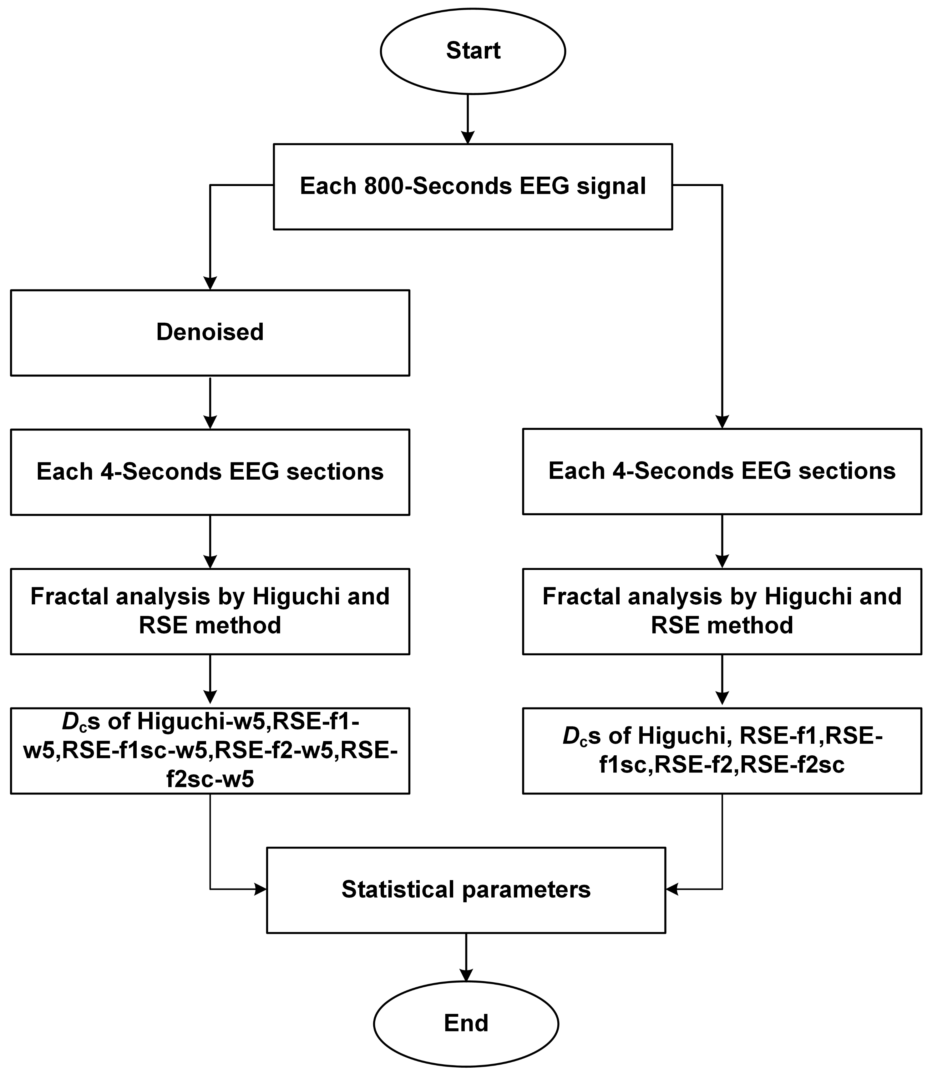
The calculation flowchart of fractal analysis on epileptic EEG signals was illustrated in Figure 1. All the above algorithms (Higuchi, RSE-f1, RSE-f1sc, RSE-f2 and RSE-f2sc) would be used on both the raw and denoised signals to obtain the calculated fractal dimension ($D_{\mathrm{c}}$) values. The denoised process used in this study included the filtering with a passband of 0.7–45 Hz and the 5-layered wavelet decomposition. The $D_{\mathrm{c}}$ values obtained by the same algorithms were suffixed by “w5” to indicate the denoising process.

3. Results and Discussion

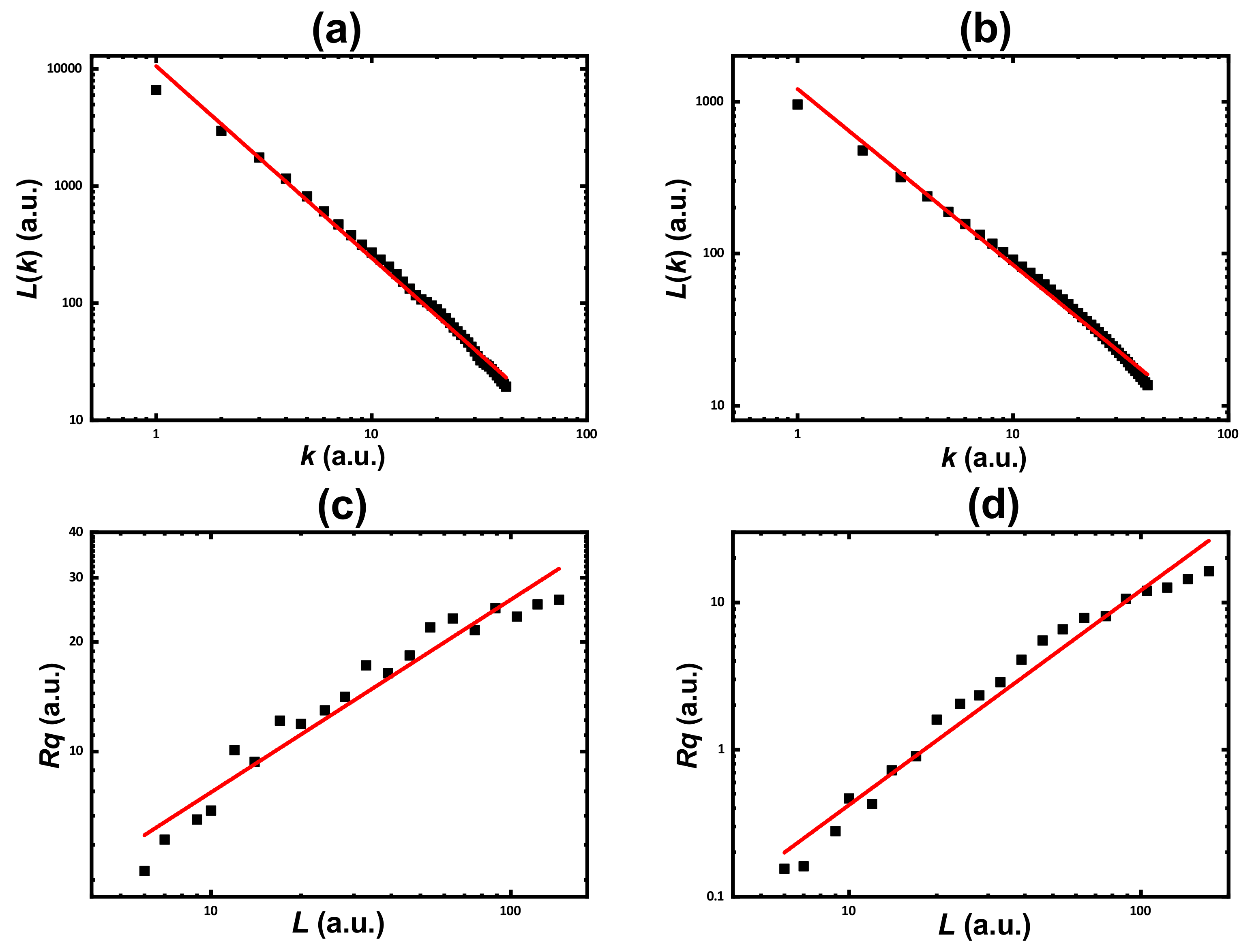
All 109 groups of 800-s EEG signals were analyzed by using Higuchi and RSE algorithms. The double logarithmic plots were shown in Figure 2, including the typical curves of raw and denoised signal with Higuchi and RSE-f1 algorithm.

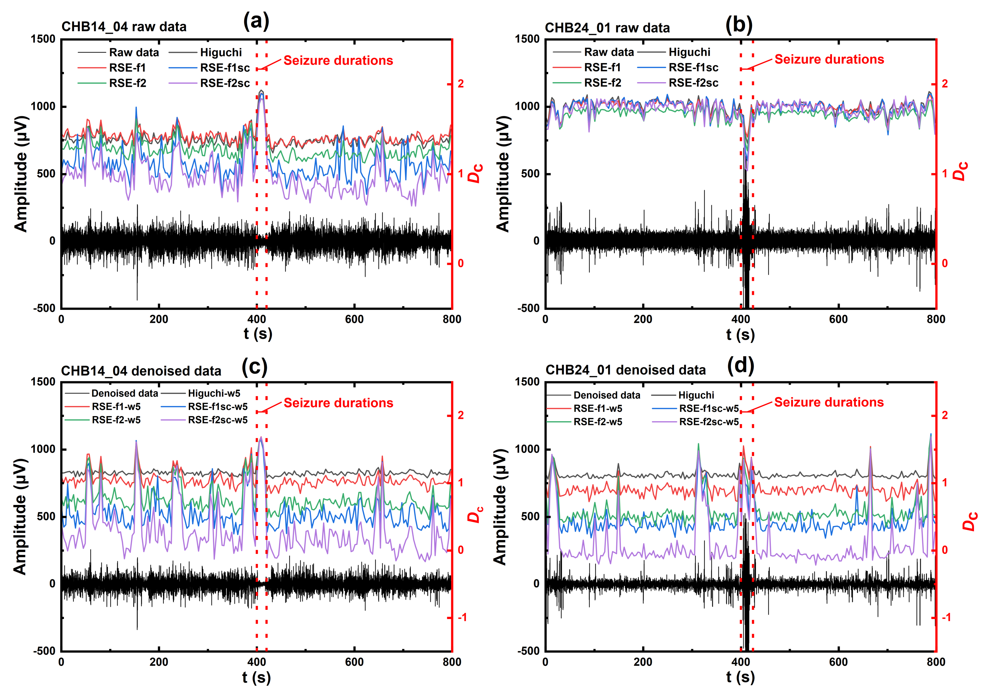
The typical EEG signals from raw and denoised data with seizure onset and the corresponding $D_{\mathrm{c}}$ values were shown in Figure 3. The results of the raw data of CHB14_04 and CHB24_01 could be observed in Figure 3a,b, respectively. In the seizure status, $D_{\mathrm{c}}$ was increased in CHB14_04 but decreased in CHB24_01. However, all $D_{\mathrm{c}}$ were increased in the seizure status after denoising, as shown in Figure 3c,d.

It should be noted that the variation of $D_{\mathrm{c}}$ values between seizure and normal statuses obtained by using Higuchi algorithm was the least obvious, while that of RSE-f2sc algorithm was the most obvious, enabling the effective distinguishing of different status based on $D_{\mathrm{c}}$ values. The more obvious variation of RSE-f2sc algorithm could be attributed to the influence of scaling region interception method. The $D_{\mathrm{c}}$ values of RSE-f1sc and RSE-f2sc could be below 1 in the normal status, which indicate that the non-fractal nature of EEG signals during normal status. In our recent publication [23], it had been demonstrated that only RSE algorithm could quantify the complexity of non-fractal features, and there could be a continuity of $D_{\mathrm{c}}$ variation across fractal and non-fractal.

It was generally regarded that the brain activities during seizure status would become more complex. Since $D_{\mathrm{c}}$ reflect the complexity of features such as signals and surfaces, it could be inferred that $D_{\mathrm{c}}$ should be larger during seizure status [23]. However, the two opposite variation trends of $D_{\mathrm{c}}$ in Figure 3b were different, which were both found in various publications as mentioned above. It was speculated that the influence of noise was the cause for such a difference, thus the $D_{\mathrm{c}}$ values of the seizure and normal statuses for all EEG signals were compared.

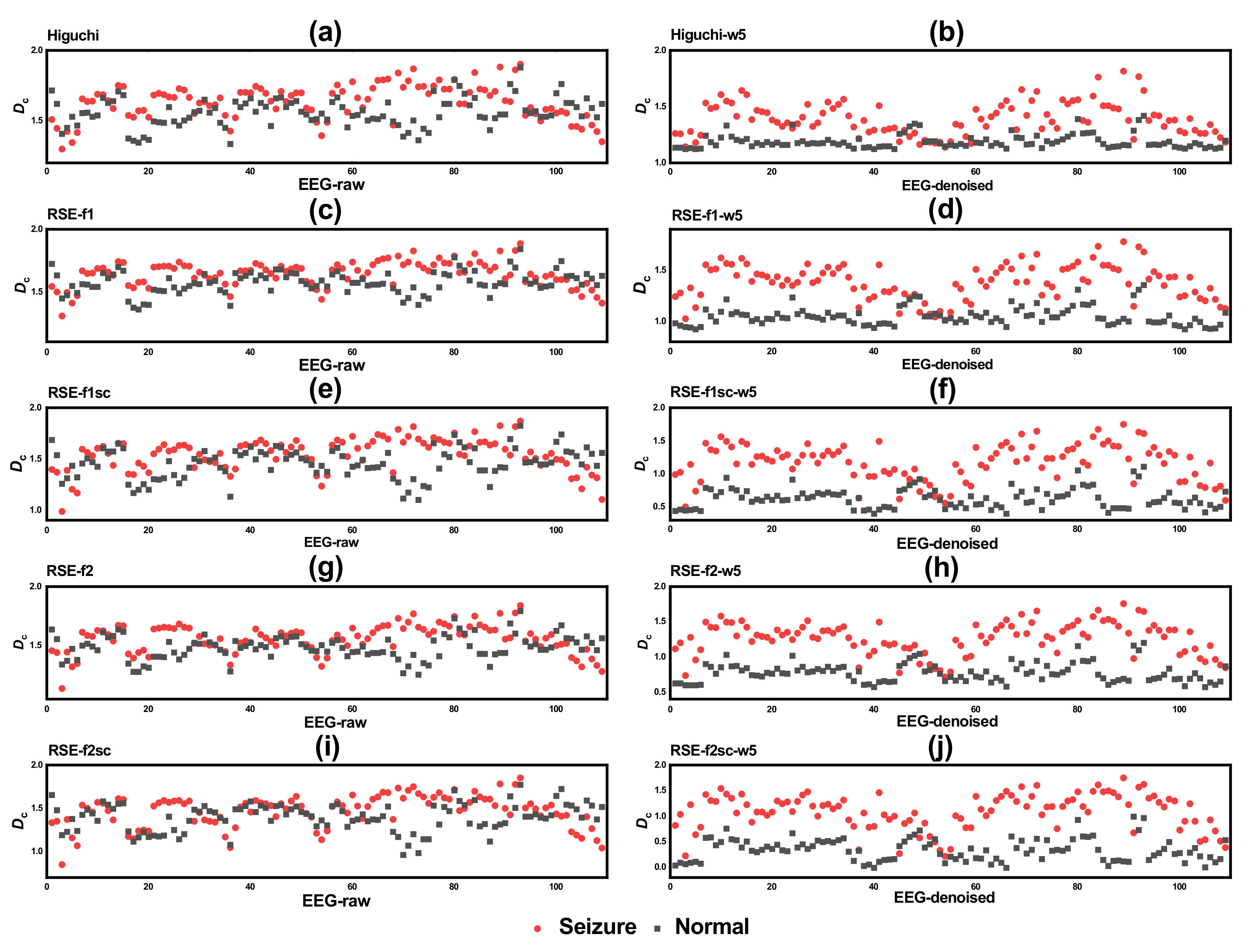
The fractal analysis on EEG signals was illustrated in Figure 4, where the 10 subfigures were the mean values of $D_{\mathrm{c}}$ by using various algorithms from all 109 groups of 800-s raw and denoised EEG signal. As shown in Figure 4, the mean values of $D_{\mathrm{c}}$ were larger in the seizure status at most groups of both raw and denoised EEG signals, and the trend was more obvious after denoising. To further analyze the influence of denoising on EEG signals based on fractal analysis, all $D_{\mathrm{c}}$ values in Figure 4 were statistically analyzed.

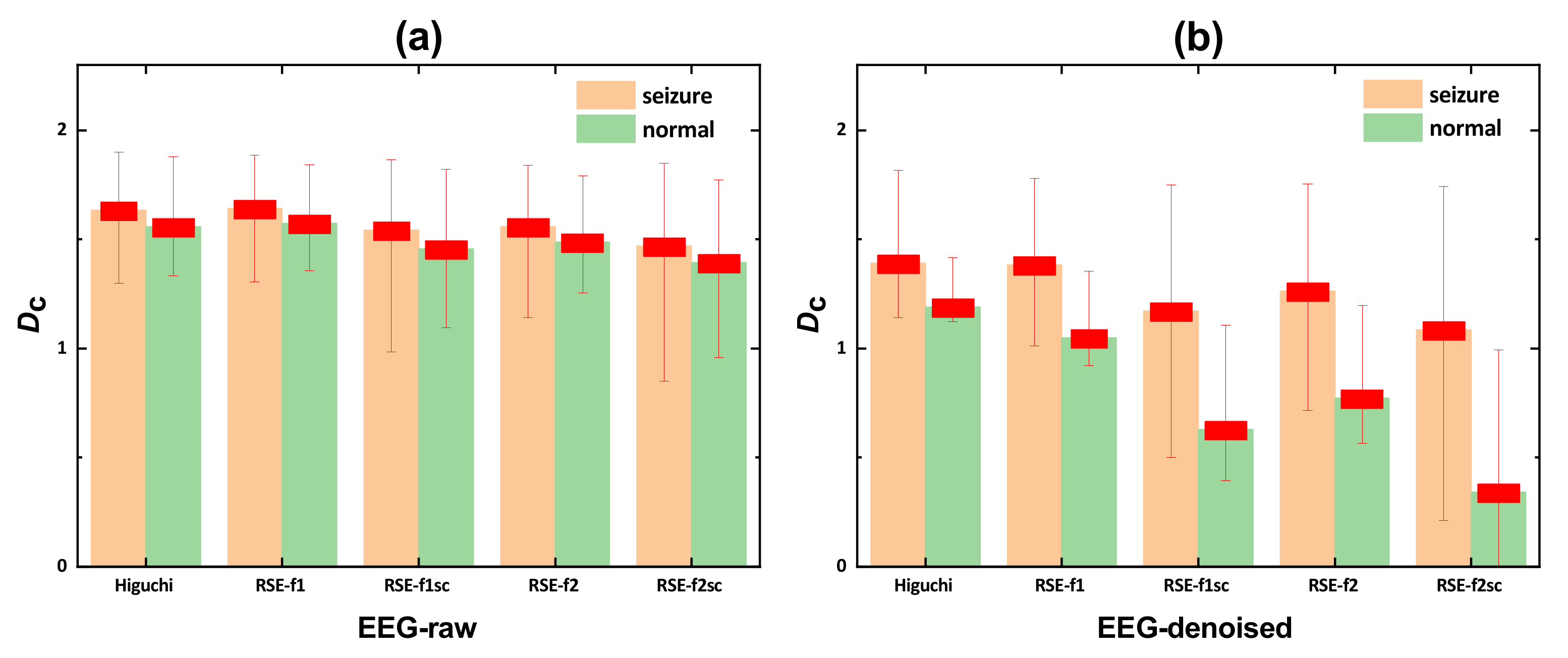
For raw EEG signals, $D_{\mathrm{c}}$ values were not much different from various algorithms between the seizure and normal statuses, and $D_{\mathrm{c}}$ values of the seizure status were generally larger. The $D_{\mathrm{c}}$ values of RSE-f1 were the largest while those of RSE-f2sc were the lowest, and all $D_{\mathrm{c}}$ values were above 1, as shown in Figure 5a.

After denoising, all $D_{\mathrm{c}}$ values were reduced for various algorithms. The $D_{\mathrm{c}}$ values of Higuchi were the largest, and those of RSE-f2sc were the lowest. $D_{\mathrm{c}}$ values were below 1 in the seizure status of RSE-f1sc, RSE-f2 and RSE-f2sc algorithms, as shown in Figure 5b. For the RSE algorithm, the $D_{\mathrm{c}}$ values became lower after using the scaling region interception method. Meanwhile, Figure 5b showed higher absolute differences between seizure and normal statuses but also larger error bars. However, the corresponding standard deviation was small, which meant that the error bars come from few data, the distribution of the overall data tended to the mean value. Additionally, the values of $D_{\mathrm{c}}$ difference between seizure and normal statuses became larger under the same algorithm after being denoised. Therefore, the statistical analysis on the $D_{\mathrm{c}}$ difference needed to be conducted to further illustrate the effect of noise reduction, the values of $D_{\mathrm{c}}$ difference were divided into ten groups under various algorithms of raw and denoised signals, respectively.

First, the distribution of each group was tested, where the Shapiro–Wilk test in R language was used (Shapiro–Wilk normality test, shapiro.test), the results were summarized in

Table 2. Shapiro–Wilk test results of the values of $D_{\mathrm{c}}$ difference between seizure and normal statuses.

Data	Algorithm	W	p-Value
EEG-raw	Higuchi	0.98944	5.58 × 10${}^{-1}$
	RSE-f1	0.98895	5.18 × 10${}^{-1}$
	RSE-f1sc	0.98831	4.68 × 10${}^{-1}$
	RSE-f2	0.98811	4.52 × 10${}^{-1}$
	RSE-f2sc	0.98258	1.66 × 10${}^{-1}$
EEG-denoised	Higuchi	0.98921	5.39 × 10${}^{-1}$
	RSE-f1	0.96064	2.65 × 10${}^{-3}$
	RSE-f1sc	0.96723	8.68 × 10${}^{-3}$
	RSE-f2	0.95819	1.74 × 10${}^{-3}$
	RSE-f2sc	0.97522	3.95 × 10${}^{-2}$

, which was mainly used to test the normal distribution of $D_{\mathrm{c}}$ differences value between seizure and normal statuses [39]. W and p-value are the test statistic, and the null hypothesis of this test is that the sample is originated from a normally distributed parent. When p-value is less than the selected significance level (usually 0.05), the null hypothesis is rejected. As shown in Table 2, not all of the ten groups were normally distributed with a significance level below 0.05, therefore the $D_{\mathrm{c}}$ difference of the same algorithm between raw and denoised signals were tested with Wilcoxon Two-sample Rank sum test.

Second, since each group was independent, the different groups of the same algorithm were paired data, the commonly used Wilcoxon Two-sample Rank sum test in R language was used to test the difference between groups (Wilcoxon rank sum test, Wilcox.test) [40]. W and p-value are the test statistic, when p-value is less than the selected significance level (usually 0.05), the $D_{\mathrm{c}}$ difference value of the two groups are considered to be significantly different. As shown in

Table 3. Willcoxon Two-sample Rank sum test results between the different groups (raw and denoised signals).

Algorithm	W	p-Value
Higuchi	8733	2.02 × 10${}^{-9}$
RSE-f1	10553	<2.2 × 10${}^{-16}$
RSE-f1sc	10631	<2.2 × 10${}^{-16}$
RSE-f2	10909	<2.2 × 10${}^{-16}$
RSE-f2sc	10985	<2.2 × 10${}^{-16}$

, the p-value of each algorithm was less than 3 × 10${}^{-3}$, revealing the highly distinguished differences between seizure and normal statuses under the same algorithm after denoising, and the results were consistent with Figure 4 and Figure 5.

The results from Figure 3, Figure 4 and Figure 5 and Table 2 and Table 3 indicated that the noise had a great influence on fractal analysis of EEG signals. After denoising, $D_{\mathrm{c}}$ values calculated by various algorithms could better distinguish the seizure status, the difference between the seizure and normal statuses could be more significant. After using the scaling region interception method, the RSE algorithm had a better performance in seizure detection.

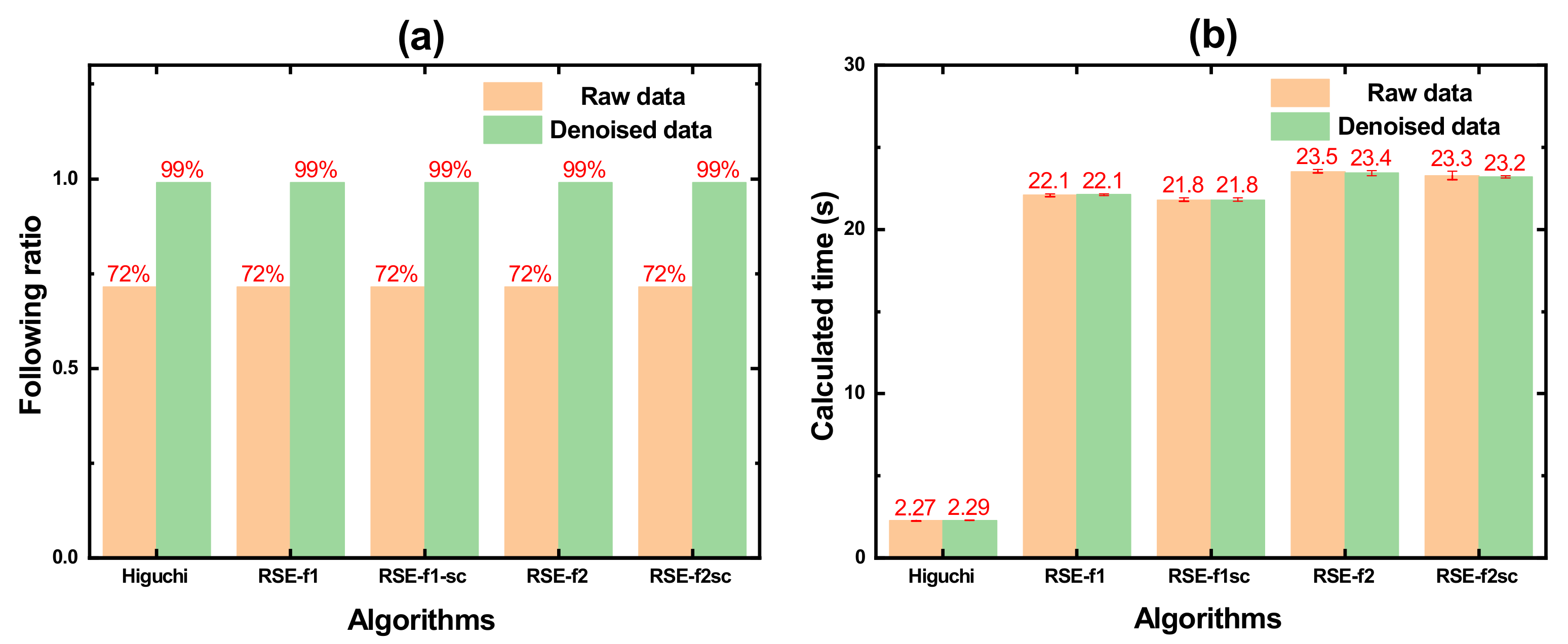
In addition to the above results, since the $D_{\mathrm{c}}$ values should reflect the complexity of the corresponding segmenting signal, i.e., theoretically the $D_{\mathrm{c}}$ should increase when epilepsy occurred, the following ratio was used to compare the differences among various algorithms. In this study, the following ratio meant the percentage of $D_{\mathrm{c}}$ increasing in the seizure status. The following ratios was 72% for raw signals of all algorithms as illustrated in Figure 6a. After denoising, all following ratios of various algorithms could reach 99%, which meant that the noise indeed had an obvious influence on the fractal analysis of EEG signals, particularly on the variation trends of $D_{\mathrm{c}}$ in seizure status.

In practical application, the calculation speed of the algorithm also needed to be considered. The calculation times of one group of EEG signals were calculated by various algorithms of raw and denoised signals, as shown in Figure 6b. The calculated times were almost the same between raw and denoised EEG signals among various algorithms. Compared with all algorithms, the Higuchi algorithm had the shortest calculated time, while the RSE-f2 algorithm had the longest. The RSE algorithm would be shorter a little after using the scaling region interception method, however, all kinds of RSE algorithms were longer than 20 s. Higuchi algorithm, by contrast, had the shortest computing time, but its $D_{\mathrm{c}}$ accuracy and variation significance were not as high as RSE algorithm. In order to achieve a real-time monitoring, all the factors of high speed, $D_{\mathrm{c}}$ accuracy and variation significance should be considered. In our future work, RSE algorithm would be accelerated significantly by using an optimizing scheme, and the feasibility of artificial neural network [41] for fractal analysis on EEG signals would be also investigated.

Besides, for the variation trends of fractal dimension in epileptic EEG signals, more data of EEG signals need to be collected, other denoising algorithms like EMD and fractal algorithms like Box-counting need to be used to further verify the universality and necessity of the noise reduction. The results of this study fully illustrated the influence of denoising process on EEG signal and seizure recognition, and provided a general template for studying the influence of specific signals not limited to EEG signal before and after noise reduction, and provided a reference for future signal process and device development.

4. Conclusions

In this study, two opposite variation trends of fractal dimension in epileptic EEG signals were demonstrated, which could both be consistent with the literature, and the influences of denoising process were analyzed. Higuchi and RSE (RSE-f1, RSE-f1sc, RSE-f2 and RSE-f2sc) algorithms were used to calculate the $D_{\mathrm{c}}$ values of the EEG signals. Based on the CHB-MIT Scalp EEG database, 109 groups of EEG signals which met the 800-s requirement and had the correct epileptic seizures status were employed to carry out the comparative study. The $D_{\mathrm{c}}$ values of the seizure and normal statuses were calculated by using various algorithms of raw and denoised signals. To further illustrate the influences of denoising, the following ratio and calculated time were also compared. This study would be promising to help to make more understandings of the nonlinear nature and scaling property of EEG signals. The conclusions of this study could be summarized as follows:

• $D_{\mathrm{c}}$ could quantify the complexity of EEG signals, and the noise had a significant influence on $D_{\mathrm{c}}$ variation trends of EEG signals. After denoised, the following ratio calculated by all algorithms could be increased from 72% to 99%;
• After using the scaling region interception method, $D_{\mathrm{c}}$ obtained by RSE-f1sc and RSE-f2sc were more favorable to distinguish the seizure status from normal status, because $D_{\mathrm{c}}$ values in normal status were generally below 1, which indicated the non-fractal nature of EEG signals in such cases. The capability of RSE algorithm to quantify the complexity of non-fractal features could be promising for the analysis on EEG signals. The underlying mechanism of RSE algorithm and the fractal nature of EEG signals in more clinical events would be investigated in our future study.

References

- Gabard, D.L.J.; Wilkinson, C.; Kapur, K.; Tager, F.H.; Levin, A.R.; Nelson, C.A. Longitudinal EEG power in the first postnatal year differentiates autism outcomes. Nat. Commun. 2019, 10, 4188. [Google Scholar] [CrossRef]
- Wu, W.; Zhang, Y.; Jiang, J.; Lucas, M.V.; Fonzo, G.A.; Rolle, C.E.; Cooper, C.; Chin, F.C.; Krepel, N.; Cornelssen, C.A.; et al. An electroencephalographic signature predicts antidepressant response in major depression. Nat. Biotechnol. 2020, 38, 439–447. [Google Scholar] [CrossRef]
- Nilsonne, G.; Harrell, F.E. EEG-based model and antidepressant response. Nat. Biotechnol. 2021, 39, 27. [Google Scholar] [CrossRef]
- Seeber, M.; Cantonas, L.M.; Hoevels, M.; Sesia, T.; Visser, V.V.; Michel, C.M. Subcortical electrophysiological activity is detectable with high-density EEG source imaging. Nat. Commun. 2019, 10, 753. [Google Scholar] [CrossRef] [Green Version]
- Soekadar, S.R.; Witkowski, M.; Gómez, C.; Opisso, E.; Medina, J.; Cortese, M.; Cempini, M.; Carrozza, M.C.; Cohen, L.G.; Birbaumer, N.; et al. Hybrid EEG/EOG-based brain/neural hand exoskeleton restores fully independent daily living activities after quadriplegia. Sci. Robot. 2016, 1, eaag3296. [Google Scholar] [CrossRef] [PubMed] [Green Version]
- Zflores, E.; Trujillo, L.; Legrand, P.; Faïta, A.F. EEG Feature Extraction Using Genetic Programming for the Classification of Mental States. Algorithms 2020, 13, 221. [Google Scholar] [CrossRef]
- Zahedi, A.; Stuermer, B.; Hatami, J.; Rostami, R.; Sommer, W. Eliminating stroop effects with post-hypnotic instructions: Brain mechanisms inferred from EEG. Neuropsychologia 2017, 96, 70–77. [Google Scholar] [CrossRef] [PubMed]
- Ciprian, C.; Masychev, K.; Ravan, M.; Manimaran, A.; Deshmukh, A. Diagnosing Schizophrenia Using Effective Connectivity of Resting-State EEG Data. Algorithms 2021, 14, 139. [Google Scholar] [CrossRef]
- Klassen, B.T.; Hentz, J.G.; Shill, H.A.; Driver-Dunckley, E.; Evidente, V.G.H.; Sabbagh, M.N.; Adler, C.H.; Caviness, J.N. Quantitative EEG as a predictive biomarker for Parkinson disease dementia. Neurology 2011, 77, 118–124. [Google Scholar] [CrossRef] [PubMed] [Green Version]
- Purnamasari, P.; Ratna, A.; Kusumoputro, B. Development of Filtered Bispectrum for EEG Signal Feature Extraction in Automatic Emotion Recognition Using Artificial Neural Networks. Algorithms 2017, 10, 63. [Google Scholar] [CrossRef]
- Murugappan, M.; Ramachandran, N.; Sazali, Y. Classification of human emotion from EEG using discrete wavelet transform. J. Biomed. Sci. Eng. 2010, 3, 390–396. [Google Scholar] [CrossRef] [Green Version]
- Jenke, R.; Peer, A.; Buss, M. Feature Extraction and Selection for Emotion Recognition from EEG. IEEE Trans. Affect. Comput. 2014, 5, 327–339. [Google Scholar] [CrossRef]
- Ravan, M. A machine learning approach using EEG signals to measure sleep quality. AIMS Electron. Electr. Eng. 2019, 3, 347–358. [Google Scholar] [CrossRef]
- Aldayel, M.; Ykhlef, M.; Al-Nafjan, A. Recognition of Consumer Preference by Analysis and Classification EEG Signals. Front. Hum. Neurosci. 2021, 14, 560. [Google Scholar] [CrossRef] [PubMed]
- Damaševičius, R.; Maskeliūnas, R.; Kazanavičius, E.; Woźniak, M. Combining Cryptography with EEG Biometrics. Comput. Intell. Neurosci. 2018, 2018, 1867548. [Google Scholar] [CrossRef] [PubMed] [Green Version]
- Martišius, I.; Damaševičius, R. A Prototype SSVEP Based Real Time BCI Gaming System. Comput. Intell. Neurosci. 2016, 2016, 3861425. [Google Scholar] [CrossRef] [Green Version]
- Lachaux, J.P.; Axmacher, N.; Mormann, F.; Halgren, E.; Crone, N.E. High-frequency neural activity and human cognition: Past, present and possible future of intracranial EEG research. Prog. Neurobiol. 2012, 98, 279–301. [Google Scholar] [CrossRef] [Green Version]
- Yuan, Q.; Zhou, W.; Liu, Y.; Wang, J. Epileptic Seizure detection with linear and nonlinear features. Epilepsy Behav. 2012, 24, 415–421. [Google Scholar] [CrossRef] [PubMed]
- Paramanathan, P.; Uthayakumar, R. Application of fractal theory in analysis of human electroencephalographic signals. Comput. Biol. Med. 2008, 38, 372–378. [Google Scholar] [CrossRef] [PubMed]
- Kesic, S.; Spasic, S.Z. Application of Higuchi’s fractal dimension from basic to clinical neurophysiology: A review. Comput. Meth. Prog. Bio. 2016, 133, 55–70. [Google Scholar] [CrossRef] [PubMed]
- Khoa, T.Q.; Ha, V.Q.; Toi, V.V. Higuchi fractal properties of onset epilepsy electroencephalogram. Comput. Math. Methods Med. 2012, 2012, 461426. [Google Scholar] [CrossRef] [Green Version]
- Wang, S.; Zhang, J.; Feng, F.; Qian, X.; Jiang, L.; Huang, J.; Liu, B.; Li, J.; Xia, Y.; Feng, P. Fractal Analysis on Artificial Profiles and Electroencephalography Signals by Roughness Scaling Extraction Algorithm. IEEE Access 2019, 7, 89265–89277. [Google Scholar] [CrossRef]
- Li, Z.; Qian, X.; Feng, F.; Qu, T.; Xia, Y.; Zhou, W. A Continuous Variation of Roughness Scaling Characteristics across Fractal and Non-Fractal Profiles. Fractals 2021, 29, 2150109-638. [Google Scholar] [CrossRef]
- Zhang, Y.; Zhou, W.; Yuan, S.; Yuan, Q. Seizure detection method based on fractal dimension and gradient boosting. Epilepsy Behav. 2015, 43, 30–38. [Google Scholar] [CrossRef] [PubMed]
- Polychronaki, G.E.; Ktonas, P.Y.; Gatzonis, S.; Siatouni, A.; Asvestas, P.A.; Tsekou, H.; Sakas, D.; Nikita, K.S. Comparison of fractal dimension estimation algorithms for epileptic seizure onset detection. J. Neural Eng. 2010, 7, 046007. [Google Scholar] [CrossRef]
- Esteller, R.; Vachtsevanos, G.; Echauz, J.; Litt, B. A comparison of waveform fractal dimension algorithms. IEEE Trans. Circuits Syst. I Fundam. Theory Appl. 2001, 48, 177–183. [Google Scholar] [CrossRef] [Green Version]
- Esteller, R.; Vachtsevanos, G.; Echauz, J.; Lilt, B. A comparison of fractal dimension algorithms using synthetic and experimental data. In Proceedings of the 1999 IEEE International Symposium on Circuits and Systems, Orlando, FL, USA, 30 May–2 June 1999. [Google Scholar]
- Romo, V.R.; Vélez, P.H.; Ranta, R.; Louis, D.V.; Maquin, D.; Maillard, L. Blind source separation, wavelet denoising and discriminant analysis for EEG artefacts and noise cancelling. Biomed. Signal Process. Control 2012, 7, 389–400. [Google Scholar] [CrossRef] [Green Version]
- Kalpakam, N.V.; Venkataramanan, S. Haar wavelet decomposition of EEG signal for ocular artifact denoising: A mathematical analysis. In Proceedings of the 2nd Annu IEEE N W Circ Syst NEWCAS 2004, Montreal, QC, Canada, 23–23 June 2004; pp. 141–144. [Google Scholar]
- Sharma, R.; Pachori, R.B. Classification of epileptic seizures in EEG signals based on phase space representation of intrinsic mode functions. Expert Syst. Appl. 2015, 42, 1106–1117. [Google Scholar] [CrossRef]
- Sweeney-Reed, C.M.; Nasuto, S.J. A novel approach to the detection of synchronisation in EEG based on empirical mode decomposition. J. Comput. Neurosci. 2007, 23, 79–111. [Google Scholar] [CrossRef] [PubMed]
- Shoeb, A. Application of Machine Learning to Epileptic Seizure Onset Detection and Treatment. Ph.D. Thesis, Massachusetts Institute of Technology, Cambridge, MA, USA, 2009. [Google Scholar]
- Goldberger, A.L.; Amaral, L.A.; Glass, L.; Hausdorff, J.M.; Ivanov, P.C.; Mark, R.G.; Mietus, J.E.; Moody, G.B.; Peng, C.K.; Stanley, H.E. PhysioBank, PhysioToolkit, and PhysioNet: Components of a new research resource for complex physiologic signals. Circulation 2000, 101, E215–E220. [Google Scholar] [CrossRef] [Green Version]
- Mansouri, A.; Singh, S.P.; Sayood, K. Online EEG Seizure Detection and Localization. Algorithms 2019, 12, 176. [Google Scholar] [CrossRef] [Green Version]
- Higuchi, T. Approach to an irregular time series on the basis of the fractal theory. Physica D 1988, 31, 277–283. [Google Scholar] [CrossRef]
- Gomez, C.; Mediavilla, A.; Hornero, R.; Abasolo, D.; Fernandez, A. Use of the Higuchi’s fractal dimension for the analysis of MEG recordings from Alzheimer’s disease patients. Med. Eng. Phys. 2009, 31, 306–313. [Google Scholar] [CrossRef] [PubMed] [Green Version]
- Bachmann, M.; Lass, J.; Suhhova, A.; Hinrikus, H. Spectral asymmetry and Higuchi’s fractal dimension measures of depression electroencephalogram. Comput. Math. Methods Med. 2013, 2013, 251638. [Google Scholar] [CrossRef] [PubMed] [Green Version]
- Xia, Y.S.; Feng, P.F.; Qian, X.; X., M.Z.; Li, Z.W.; Zhou, W.M.; Feng, F. Properties and benefits of scaling region in fractal analysis by using roughness scaling extraction algorithm. Pattern Recognit. 2021. under review. [Google Scholar]
- Shapiro, S.S.; Wilk, M.B. An analysis of variance test for normality. Biometrika 1965, 52, 591–611. [Google Scholar] [CrossRef]
- Roussas, G.G. An Introduction to Probability and Statistical Inference; Elsevier: London, UK, 2015. [Google Scholar]
- Zhou, G.; Wang, X.; Feng, F.; Feng, P.; Zhang, M. Calculation of fractal dimension based on artificial neural network and its application for machined surfaces. Fractals 2021, 29, 2150129. [Google Scholar] [CrossRef]