Load Balancing Strategies for Slice-Based Parallel Versions of JEM Video Encoder

Abstract

The proportion of video traffic on the internet is expected to reach 82% by 2022, mainly due to the increasing number of consumers and the emergence of new video formats with more demanding features (depth, resolution, multiview, 360, etc.). Efforts are therefore being made to constantly improve video compression standards to minimize the necessary bandwidth while retaining high video quality levels. In this context, the Joint Collaborative Team on Video Coding has been analyzing new video coding technologies to improve the compression efficiency with respect to the HEVC video coding standard. A software package known as the Joint Exploration Test Model has been proposed to implement and evaluate new video coding tools. In this work, we present parallel versions of the JEM encoder that are particularly suited for shared memory platforms, and can significantly reduce its huge computational complexity. The proposed parallel algorithms are shown to achieve high levels of parallel efficiency. In particular, in the All Intra coding mode, the best of our proposed parallel versions achieves an average efficiency value of 93.4%. They also had high levels of scalability, as shown by the inclusion of an automatic load balancing mechanism.

1. Introduction

The High Efficiency Video Coding (HEVC) standard [1] was developed by the Joint Collaborative Team on Video Coding (JCT-VC) in 2013, and replaced the previous H.264/Advanced Video Coding (AVC) standard [2]. The HEVC standard obtains savings in terms of bit rate of almost 50%, with the same visual quality as the previous H.264/AVC standard. However, this reduction is obtained at the expense of a huge increase in the computational complexity of the encoding process [3].

Recently, Cisco released a report called “Forecast and Trends: 2017–2022 White Paper” [4], in which they state that IP video traffic will form 82% of all IP traffic by 2022, representing a four-fold increase between 2017 and 2022. This represents a situation where each second, a million minutes of video content travel through the network. The report also predicts a constant increase in novel services such as video-on-demand (VoD), live internet video, virtual reality (VR) and augmented reality (AR). VoD traffic is expected to double by 2022, mainly due to the increasing numbers of consumers and higher video resolution (4 K and 8 K), bringing the amount of VoD traffic to the equivalent of 10 billion DVDs per month. The impact of user devices on global traffic is even more important when we consider popular services such as ultra-high-definition (UHD) video streaming. We need to take into account the fact that the bit rate for 4 K video is about 15 to 18 Mbps, more than double the bit rate for HD video and nine times more than standard definition (SD) video. The Cisco report estimates that by 2022, nearly 62% of the flat-panel TV sets installed will be UHD.

In order to deal with this increase in IP video traffic, new video coding techniques are required to obtain higher compression rates. Since the release of HEVC, both the ITU-T Video Coding Expert Group (VCEG) and the ISO/IEC Moving Picture Expert Group (MPEG) have been studying and analyzing new video coding technologies in order to improve the compression capability compared to that obtained by HEVC. To achieve this, a framework of collaboration has been created called the Joint Video Exploration Team (JVET).

The compression enhancements studied by the JVET have been implemented in a software package known as the Joint Exploration test Model (JEM) [5]. Its main purpose is to explore new coding tools that can provide significant improvements at the video coding layer. Following an analysis of the new coding tools that have been proposed within the last few years, JVET has begun developing a future video coding standard called Versatile Video Coding (VVC) [6]. The main goal of this coding standard is to achieve bit rate savings of between 25% and 30% compared to HEVC [7,8].

Preliminary results obtained with the new model (JEM 3.0) show an 18% reduction in bit rate using the All Intra (AI) coding mode configuration [9]. However, this is achieved at the expense of an extremely large increase in computational complexity (60x) with respect to HEVC.

This increase requires the introduction of acceleration techniques that leverage hardware architectures to reduce encoding time. Since JEM is an exploration model, only a few articles have been published on the subject, and most of them are focused on rate distortion (R/D) comparisons between JEM, HEVC and AV1 codecs [10]. Recently, the authors of [11] proposed a pre-analysis algorithm that was designed to extract motion information from a frame in order to accelerate the motion estimation (ME) stage. Their proposal showed that around 27% of the reference frames could be skipped, and that a time saving of more than 62% was achieved on the integer ME operation, with a negligible impact of 0.11% on the Bjøntegaard delta rate (BD rate) [12]. The authors in [13] proposed parallel algorithms based on the group of pictures (GOP) structure, increasing the BD rate when temporal redundancy is exploited.

In this paper, we present two JEM parallel encoder versions that are specifically designed for shared memory platforms, in order to speed up the encoding process for the All Intra (AI) coding mode, as this coding mode is especially useful for video editing. We performed several experimental tests to illustrate the behavior of the parallel versions in terms of their parallel efficiency and scalability. In the first parallel algorithm, a synchronous algorithm named JEM-SP-Sync, a domain decomposition is performed, in which the computational load is not balanced, although the data are almost equally distributed. The second parallel algorithm, named JEM-SP-ASync, is an asynchronous algorithm, also based on a domain decomposition but able to balance the load automatically.

The rest of this paper is organized as follows. In Section 2, we present a brief description of the coding tools introduced in the new JEM video coding standard. Section 3 describes the parallel algorithms developed for the AI coding mode of the JEM standard. Experimental numerical results are presented in Section 4, and in Section 5, some conclusions are drawn.

2. Description of the New Characteristics of the Joint Exploration Test Model (JEM)

The JEM codec is based on the HEVC reference software, called HM, meaning that the overall architecture of both codecs is quite similar since they share a hybrid video codec design. However, some of the coding stages are modified in the JEM implementation in order to improve the previous standard [14,15]. The R/D performance of JEM is better than in HEVC due to the use of these techniques, but this is achieved at the expense of an increased computational cost for the intra-prediction stage. This section describes the main improvements offered by JEM in comparison to the previous standards, as these could lead to a load imbalance when using parallel algorithms such as those proposed in this work.

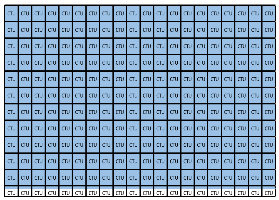
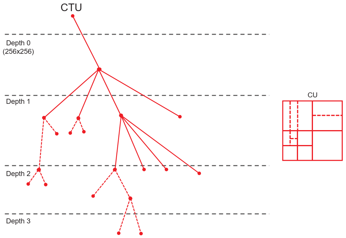
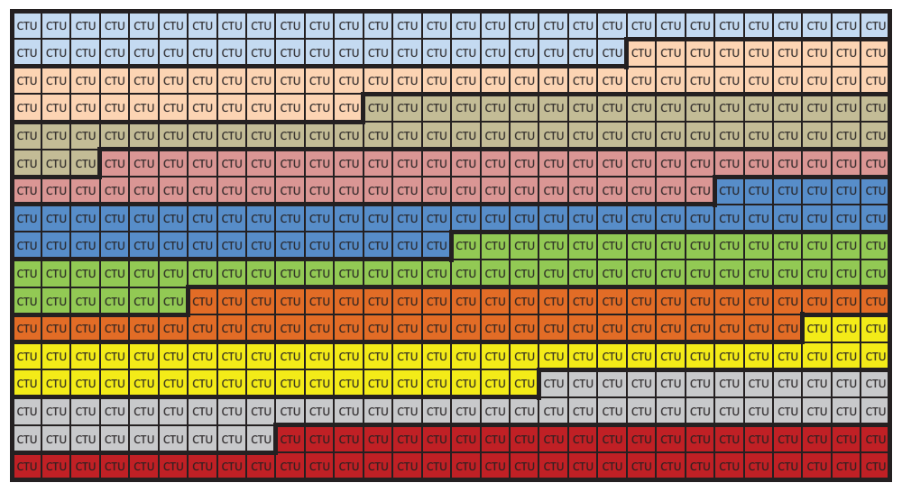
2.1. Picture Partitioning

The way in which a video frame is split into a set of non-overlapping blocks is called picture partitioning. These non-overlapping blocks are arranged into a quadtree structure, where the root is called a coding tree unit (CTU) [16], and each CTU is further partitioned into smaller blocks. Figure 1 shows the division of a $1280\times 720$ pixel frame into 240 CTUs, split into 20 columns by 12 rows, where the last row is composed of incomplete CTUs. The complete CTUs are composed of $64\times 64$ pixels.

Two of the major differences between HEVC and JEM are the way in which a CTU is further partitioned and the size of the CTU itself. In HEVC, the maximum CTU size is $64\times 64$ pixels, and there is the option to further recursively partition it into four square coding units (CU) whose sizes range from $64\times 64$ pixels (i.e., no partitioning) to $8\times 8$ pixels. The leaf blocks in a CU quadtree form the roots of two independent trees that contain prediction units (PUs) and transform units (TUs).

A PU can have the same size as the CU, or can be further split into smaller PUs of up to $8\times 8$ pixels. The PUs store the prediction information in the form of motion vectors (MVs). In intra-prediction mode, HEVC uses a quadtree structure with only square PUs, while in inter prediction mode, asymmetric splitting of PUs is possible, giving up to eight possible partitions for each PU block: 2N × 2N, 2N × N, N × 2N, N × N, 2N × nU, 2N × nD, nL × 2N and nR × 2N. 1,0,0 Figure 2 shows an example of a CTU partition in HEVC and the relationship between CU partitioning, PU partitioning and TU partitioning.

The picture partitioning schema is modified in JEM in order to simplify the prediction and transform stages, and further partitions of CUs to form PU and TU trees are avoided. The JEM partitioning schema, called quadtree plus binary tree (QTBT), offers a better match with the local characteristics of each frame [17]. The highest level is a CTU, as in HEVC, but the main change is that block splitting below each branch is a binary partition giving the leaves.

The size of the CTU is larger than in HEVC, with a maximum of $256\times 256$ pixels, and only the first partition needs to be square partitioned. Lower partitions can be partitioned further in a quadtree schema, but at the desired level the binary tree ends the partitioning schema. There are two types of splitting in the binary tree: symmetric horizontal and symmetric vertical. The binary tree leaf node is the CU, which is used for prediction and transformation with no further partitioning. Hence, in most cases, the CU, PU and TU have the same size. An example of QTBT is shown in Figure 3; here, the quadtree has two levels (continuous line), after which the binary tree starts (dotted lines).

In JEM, a CU can have either a square or a rectangular shape, and consists of coding blocks (CBs) of different color components; for example, a CU may contain one luma CB and two chroma CBs in the YUV420 chroma format.

In HEVC, inter prediction for small blocks is restricted in order to reduce memory accesses for motion compensation, i.e., bi-directional prediction for $4\times 8$ and $8\times 4$ blocks is not allowed, and $4\times 4$ inter-prediction is also disabled. In QTBT, these restrictions are removed, which increases the computational cost of the JEM codec.

The CUs are not partitioned further for transforming or prediction unless the CU is too large for the maximum transform size. The maximum transform size is $128\times 128$ pixels, which improves the coding efficiency for higher resolution video, e.g., 1080 p and 4 K sequences.

The following parameters are defined in order to obtain efficient partitioning in a QTBT tree:

• CTU size: The root node size of a quadtree; the same concept as in HEVC.
• MinQTSize: The minimum allowed size of the leaf node in the quadtree.
• MaxBTSize: The maximum allowed size of the root node in the binary tree.
• MaxBTDepth: The maximum allowed depth of the binary tree.
• MinBTSize: The minimum allowed size of the leaf node in the binary tree.

MaxBTSize and minQTSize are two factors that are critical to the R/D performance and the encoding time. In JEM, these two parameters of the current slice are set adaptively larger when the average CU size of the previous encoded picture is larger, and vice versa for only the P and B slices [17].

At the transform stage, only the lower-frequency coefficients are maintained for transform blocks with sizes (width or height) larger than or equal to 64. For example, for an M × N transform block (where M is the width and N the height), when M is larger than or equal to 64, only the left M/2 columns of transform coefficients are retained. Similarly, when N is larger than or equal to 64, only the top N/2 rows of the transform coefficients are retained. This behavior can be skipped using skip mode for large blocks.

The proposed QTBT approach in JEM uses more partition types than HEVC in order to adapt the resulting partition tree to the contents of the scene. It is guided in this task by a trade-off between rate reduction and distortion reduction, and as we will see in the next section, this is a computationally expensive task. The whole video frame is first partitioned into equally sized (up to $256\times 256$) CTUs, and each CTU is then further partitioned into CUs based on the scene contents, i.e., the time needed to process a whole CTU depends on the complexity of the underlying scene in each CTU. A summary of the main differences between HEVC and JEM related to picture partitioning is shown in

Table 1. Differences between HEVC and JEM with respect to picture partitioning.

Characteristics	HEVC	JEM
CTU size	$64\times 64$	$256\times 256$
CTU partition	Quad-Tree with separate tress for CU, PU and TU	Quad-Tree+Binary-Tree QTBT (shared by CU, PU, TU)
Inter-Prediction	No bi-directional	Bi-directional allowed for $4\times 8$ and $8\times 4$ sizes
Max transform unit size	$32\times 32$	$128\times 128$

.

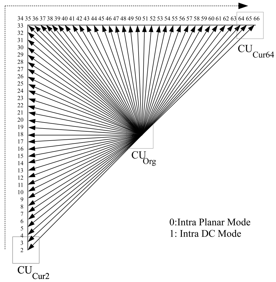
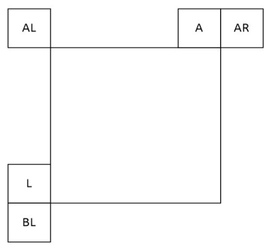
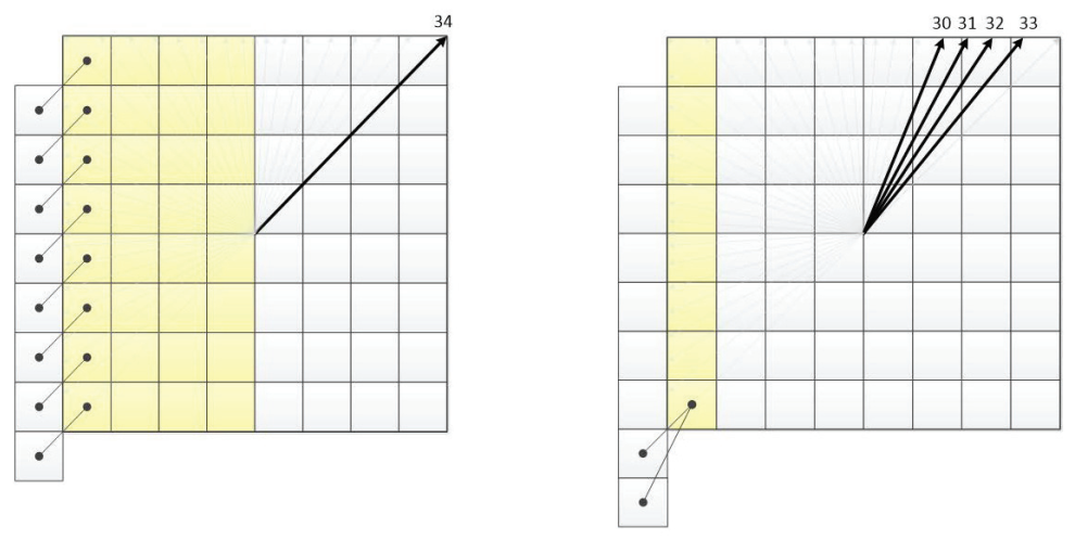
2.2. Spatial Prediction

In order to be able to capture the finer edge directions presented in natural videos, the directional intra-modes in JEM have been extended from 33, as defined in HEVC, to 65. The addition of planar and DC modes gives a total of 67 different prediction modes for JEM. These denser directional intra-prediction modes (see Figure 4) are applied to all PU sizes and both luma and chroma intra-predictions.

The partitioning schema described in the previous section is directed by a rate-distortion optimization (RDO) algorithm that recursively searches for the best possible partitioning schema in terms of an R/D estimation. This algorithm tries all directional intra-modes for each of the possible partitions, (i.e., no partitioning, vertical partitions, horizontal partitions and quadtree partitions), at each recursion level, to find the one with the lowest cost. For a CTU in which the underlying scene is smooth, this recursion ends rapidly, and the number of trials for the 67 directional modes is therefore much lower than if the CTU belongs to a highly textured area within the scene. Thus, the computational effort is not evenly distributed over the CTUs in a video frame, and depends on the content of the scene.

In JEM, the list of most probable modes (MPMs) is extended from the three used in HEVC to six, and the selection procedure for these modes is also changed. In HEVC, the method proposed in [18] was adopted in the standard for building the MPMs list. The 35 intra-modes are divided into two groups: three MPMs and 32 remaining modes. The three MPMs are derived based on the modes of the PUs to the left of and above the current PU. The new procedure followed in JEM [19] uses five neighbors of the current PU: left, above, above left, below left and above right, as shown in Figure 5 [19].

The improvements in JEM described in the following paragraphs, which increase the complexity of the encoder, can also lead to a load imbalance when parallel processing the slices of a frame.

In addition to the changes in the JEM encoder mentioned above, there are also differences in the entropy coding of the MPM list between HEVC and JEM, as explained in [17,19], which lead to a reduction of the contexts used in the entropic encoder to signal the MPM index from nine to three, corresponding to the vertical, horizontal or non-angular class MPM modes.

The interpolation filters are also changed in JEM with respect to HEVC [15]. In HEVC, a two-tap linear interpolation filter is used to generate the intra-prediction block in the directional prediction modes (i.e., excluding the planar and DC predictors). In the JEM, four-tap intra-interpolation filters are used for directional intra-prediction filtering. Cubic interpolation filters are used for blocks smaller than or equal to 64 samples, and Gaussian interpolation filters are used for larger blocks. The filter parameters are set based on the block size, and the same filter is used for all modes.

Another improvement to JEM is made in the boundary prediction filters [15]. In HEVC, after the prediction block has been generated for the vertical or horizontal intra-modes, the leftmost column or the top row of the predicted block are adjusted further using the values of the boundary samples. In JEM, the number of boundary samples is increased from one to four (rows or columns) in order to obtain the predicted value using a two-tap filter (for the first and last angular modes, corresponding to intra-modes 2 and 34 in HEVC) or a three-tap filter (for modes between intra-modes 3–6 and 30–33 in HEVC), as shown in the example in Figure 6.

In JEM, the results of the intra-prediction planar mode are also improved by including a position-dependent intra-prediction component (PDPC) method that processes a specific combination of the unfiltered boundary reference samples with the filtered ones, thus improving the perceived quality of the predicted block when the planar mode is used. This process uses different weights and filter sizes (three-tap, five-tap, seven-tap) based on the block size.

To reduce some of the redundancy that remains after the prediction process between the luma and chroma components, JEM uses cross-component linear model (CCLM) prediction. In this process, the chroma samples are predicted based on the reconstructed down-sampled luma samples of the same CU, using a linear model for square blocks. For non-square blocks, additional down-sampling is needed to match the shorter boundary. There are two CCLM modes: single- and multiple-model CCLM modes (MMLM). In the single-model CCLM mode, JEM employs only one linear model to predict the chroma samples, while in MMLM, there can be two models. In MMLM, the models are built based on two groups of boundary samples that serve as a training set for deriving the linear models [15]. A summary of the main differences between HEVC and JEM related to spatial prediction is shown in

Table 2. Differences between HEVC and JEM with respect to the spatial prediction.

Characteristics	HEVC	JEM
Intra-modes	33	67
List MPMs	3	6
N° of Neighbors for MPMs derivation	2	5
Interpolation filters	2-tap Linear	4-tap Cubic or Gaussian
Boundary filter samples	1	4

.

3. Parallel Approaches

Slices are fragments of a frame formed by correlative (in raster scan order) CTUs (see Figure 7). These are regions of the same frame that can be decoded (and also encoded) independently, which offers a valid parallelization approach for video encoding and decoding processes. However, slice independence has a drawback in that the existing redundancy between data belonging to different slices cannot be exploited, and thus the coding efficiency in terms of the R/D performance decreases. Moreover, slices are composed of a header and data, and although this is useful in terms of providing an encoded video sequence with error resilience features (since the loss of a single slice does not prevent the rest of the slices in the same frame from being properly decoded), the inclusion of a header in each slice also causes a decrease in the R/D performance.

Based on the slice partitioning of the JEM video encoder, each video frame is divided into as many slices as threads to be spawned. The number of threads in the parallel region can be set as a parameter or can be obtained depending on the current state of the computer system. Hence, the number of threads (and consequently the number of slices), and the slice size are computed before starting the encoding process. In this work, we have developed two algorithms, the first of which requires synchronization processes while the second is a completely asynchronous algorithm.

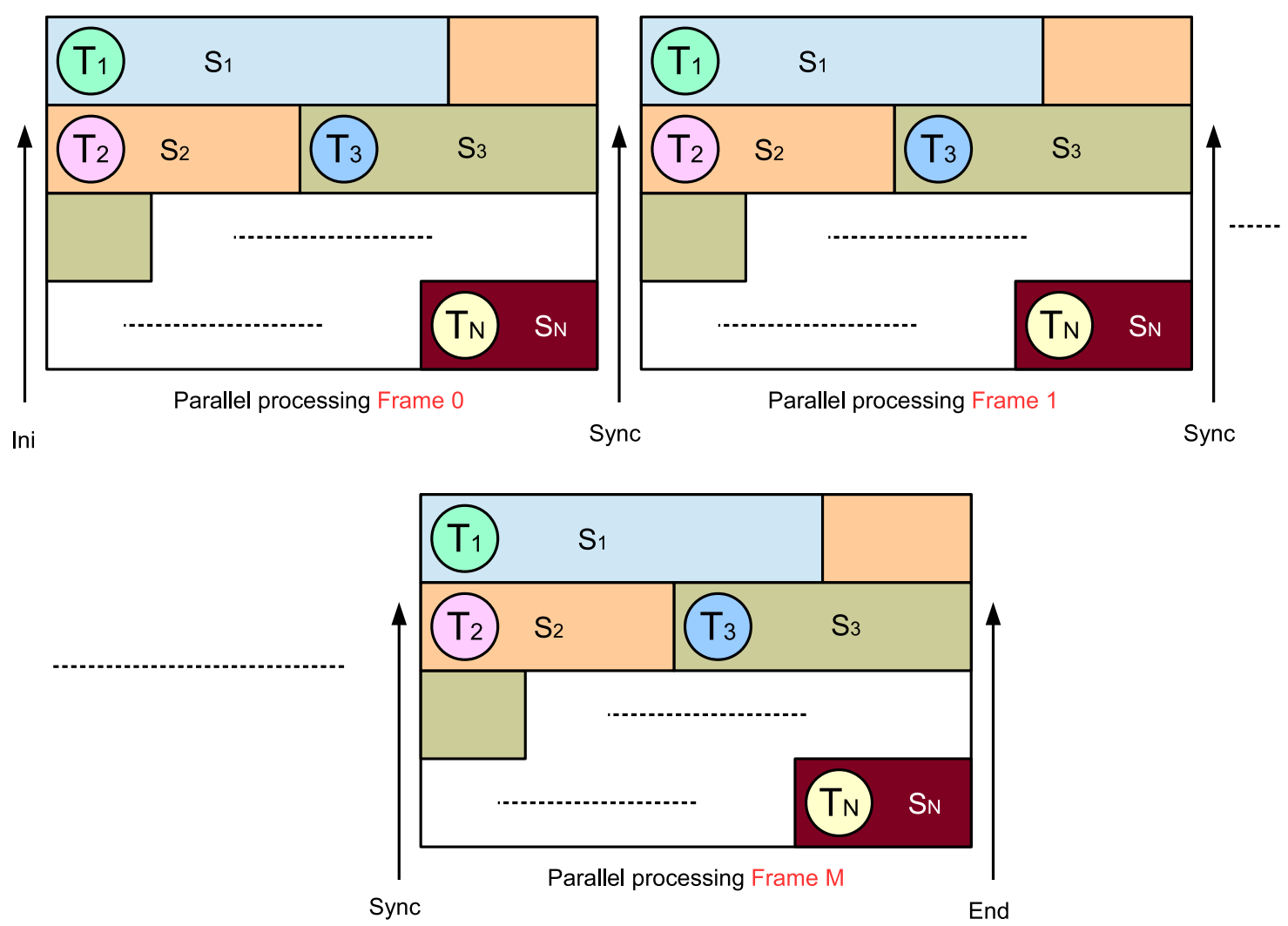
3.1. Synchronous Algorithm: JEM-SP-Sync

Algorithm 1 shows the parallel algorithm, called JEM-SP-Sync, which includes synchronization processes. In Algorithm 1, the size of the slice is first computed in numbers of CTUs. To do this, we initially compute the number of horizontal ($FrWidth$) and vertical ($FrHeight$) CTUs, and the total number of CTUs ($NoCTUs$) available in a frame, which will depend on the video resolution. It is worth noting that both the right-hand and bottom CTUs in the frame may be incomplete (see lines 4 and 8). Furthermore, since the slices may not have the same number of CTUs, the algorithm sets the size of the last slice as equal to or smaller than the size of the rest of the slices in order to achieve a better load balance (lines 13–18).

Before starting the encoding process of the whole video sequence, each thread computes the CTUs of the slice assigned to that thread, which always remains the same throughout the encoding process (lines 20–26). The encoding process starts by reading the frame to be encoded and storing it in memory. This initial process is performed by a single thread, and a synchronization point is therefore needed to ensure that the process waits until the frame is available (line 30). In a similar way, the reconstructed frame is also stored in the shared memory. This task is carried out by each individual thread after encoding the assigned slice, meaning that another synchronization point is required before applying the “loop filter” process (line 32). The encoded video data stream (i.e., the bit stream) is organized into network abstraction layer units (NALUs), where each NALU is a packet containing an integer number of bytes. To finish the encoding process, the NALUs corresponding to each slice must be written in the correct order to form the final bit stream (line 35). It is worth mentioning that the slice-based parallel strategy for HEVC proposed in [20] obtained good speed-ups when all slices had the same number of CTUs, or differed by a maximum of a single CTU. However, this behavior changes greatly when the JEM encoder is used. As explained in Section 2, changes to the coding procedure introduced in the JEM with respect to HEVC result in significant differences in computational cost when encoding different CTUs. Note that this load imbalance is mainly due to the intrinsic characteristics of the video content.

Algorithm 1 JEM-SP-Sync: Slice-based parallel algorithm with synchronization processes.

1: Set $NoT$ to the number of threads (equal to the number of slices)   2: procedure Compute the number of CTUs per frame   3:     $NoHzCTUs=FrWidth/CTUSize$   4:     if $FrWidth\%CTUSize!=0$ then   5:         $NoHzCTUs++$   6:     end if   7:     $NoVrCTUs=FrHeight/CTUSize$   8:     if $FrHeight\%CTUSize!=0$ then   9:         $NoVrCTUs++$ 10:     end if 11:     $NoCTUs=NoHzCTUs\ast NoVrCTUs$ 12: end procedure 13: procedure Compute the number of CTUs per slice 14:     $NoCTUsSlice=NoCTUs/NoThreads$ 15:     if $NoCTUs\%NoThreads!=0$ then 16:         $NoCTUsSlice++$ 17:     end if 18: end procedure 19: IN PARALLEL (NoT): 20: procedure Assign the dimms of the slice($Tid$) 21:     $iniCT{U}_{Tid}=Tid\ast NoCTUsSlice$ 22:     $endCT{U}_{Tid}=iniC{U}_{Tid}+NoCTUsSlice$ 23:     if $Tid==(NoT-1)$ then 24:         $endCT{U}_{Tid}=NoCTUs-1$ 25:     end if 26: end procedure 27: for$i=1$ to $NumFramesInSequence$ do 28:     Single thread: 29:         Read frame i it in global memory. 30:     Synchronization point #1 31:     Encode Slice ($iniCT{U}_{Tid}$ to $endCT{U}_{Tid}$) 32:     Synchronization point #2 33:     Apply the loop filter process to whole frame 34:     Generate NALUs 35:     Ordered: 36:         Write NALUS to bitstream. 37: end for

Figure 8 shows graphically the structure of the synchronous parallel algorithm JEM-SP-Sync. As explained in Algorithm 1, each thread (${\mathrm{T}}_{\mathrm{x}}$) always processes the same slice (${\mathrm{S}}_{\mathrm{x}}$) in all frames. Before starting the processing of a new frame, the threads must synchronize (Sync) to compose the bitstream of the last frame (line 35 of Algorithm 1).

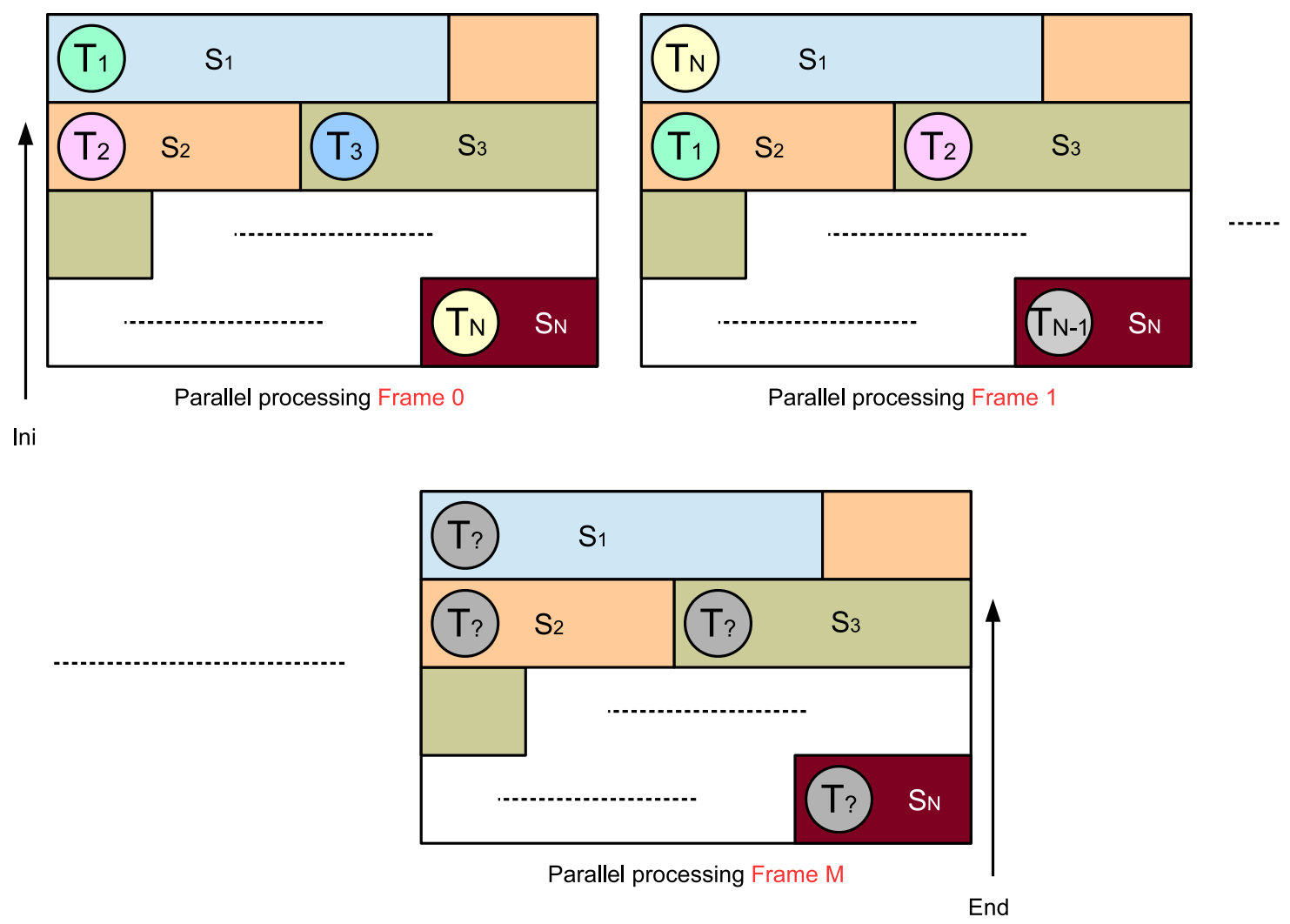
3.2. Asynchronous Algorithm: JEM-SP-ASync

To solve the load imbalance drawback, we designed a parallel algorithm called JEM-SP-ASync, as shown in Algorithm 2, which does not use any type of synchronization during the overall encoding process. The calculation of both the number of CTUs per frame and the number of CTUs per slice (line 3) is identical to that in Algorithm 1 (lines 2–18). Before starting the parallel region, the dimensions of all slices are calculated (lines 3–10) and stored in memory, which will be configured as shared memory (the iniCTUs and endCTUs arrays) since these values will be used by all threads. At the beginning of the parallel region, the first slice to be encoded by every thread is set (line 12) based on the thread identifier ($Tid$). However, the mapping of slices to threads will change for every new frame, following a round-robin-like scheduling (lines 24–27). For this reason, each thread must update the CTUs to be encoded when starting the encoding of a new frame (lines 15 and 16). Since there are no synchronization points, the encoded NALUs must be stored in shared memory.

When the encoding process for the slice is complete, each thread checks whether there is a frame for which all of the slices are encoded; if so, this thread stores the complete encoded frame in the bit stream. This procedure should be performed within a parallel critical region (lines 20–23). The proposed mapping of slices to threads included in Algorithm 2 provides an automatic load balancing mechanism without the need for synchronization points or a coordinating process. By alternating the coding slice for each thread from one frame to another, the computational cost per thread tends to balance, with a greater probability as the number of frames to be encoded increases.

In the asynchronous algorithm, shown in Figure 9, there are no synchronization points; to compose the bit stream, each thread after processing a slice checks if all the slices of the frame following the last fully encoded one are already encoded, and in that case the thread will compose that frame and remove the stored data. This process (line 17 in Algorithm 2) does not involve any synchronization point. Furthermore, each thread (${\mathrm{T}}_{\mathrm{x}}$) processes a different slice (${\mathrm{S}}_{\mathrm{x}}$) in each frame.

Algorithm 2 JEM-SP-ASync: Slice-based parallel algorithm without synchronization processes.

1: Set $NoT$ to the number of threads (equal to the number of slices)   2: $NoCTUs$ and $NoCTUsSlice$ computed as in Algorithm JEM-SP-Sync   3: procedure Compute dimmensions of all slices   4:     for $i=0$ to $(NoT-2)$ do   5:           $iniCTUs[i]=i\ast NoCTUsSlice$   6:           $endCTUs[i]=(i+1)\ast NoCTUsSlice-1$   7:     end for   8:     $iniCTUs[NoT-1]=(NoT-1)\ast NoCTUsSlice$   9:     $endCTUs[NoT-1]=NoCTUs-1$ 10: end procedure 11: IN PARALLEL (NoT): 12: $idSlice==Tid$ 13: for $i=1$ to $NumFramesInSequence$ do 14:     Read slice $idSlice$ from frame i in private memory. 15:     $currentIniCTU=iniCTUs[idSlice]$ 16:     $currentEndCTU=endCTUs[idSlice]$ 17:     Encode Slice ($currentIniCTU$ to $currentEndCTU$) 18:     Apply the loop filter process to own slice 19:     Store NALU(s) in global memory 20:     critical: 21:     if there are any fully encoded frames then 22:             Write all NALUS of that frame to bitstream. 23:     end if 24:     $idSlice++$ 25:     if $idSlice>(NoT-1)$ then 26:         $idSlice=0$ 27:     end if 28: end for

4. Experimental Results

The reference software used in our experiments was JEM-7.0rc1 [21], and the parallel algorithms were developed and tested using the GCC v.4.8.5 compiler [22] and OpenMP [23]. The shared memory platform used consisted of two Intel XEON X5660 hexacores, with up to 2.8 GHz and 12 MB cache per processor, and 48 GB of RAM. The operating system used as CentOS Linux 5.6 for x86/64-bit systems.

The proposed algorithms were tested for the video sequences listed in

Table 3. Video sequences.

Video Seq.	Acronym	Resolution	Rate (Hz)	N. Frames	Time (s)
Park Scene	PARK	1920 × 1080	24	120	5
Four People	FOUR	1280 × 720	60	120	2
Party Scene	PART	832 × 480	50	120	2.4
BQ Square	BQSQ	416 × 240	60	120	2

, each of which had a different resolution and a different frame rate. In all of the experiments, we used the same number of frames to be encoded (120) for all video sequences. Hence, the number of seconds to be encoded varied depending on the frame rate of the video sequence tested. We used a small number of frames for encoding in order to evaluate the load balancing capability of the JEM-SP-ASync algorithm (Algorithm 2). Note that as the number of frames to be encoded increases, the automatic load balancing method of Algorithm 2 is expected to improve, since it is statistically more likely that the computational cost per thread will be balanced. The values of the quantization parameter (QP) used were 37, 32, 27 and 22.

Before addressing the efficiency of the parallel algorithms described in Section 3, we analyze the theoretical load balance index, which will depend on both the resolution of the video sequence and the number of slices (i.e., the number of threads). In all of the experiments, the CTU size was set to 128, based on common testing conditions [24].

Table 4. Number of 128 × 128 CTUs for each video sequence resolution.

Resolution	Horizontal CTUs		Vertical CTUs		Number of CTUs
1920 × 1080	15	15	8.4	9	135
1280 × 720	10	10	5.6	6	60
832 × 480	6.5	7	3.8	4	28
416 × 240	3.25	4	1.9	2	8

shows the dimensions of the different video resolutions tested, in numbers of CTUs of $128\times 128$ pixels. As mentioned above, there may be incomplete CTUs at the right-hand and bottom edges of the video sequence. This occurs when the number of horizontal/vertical CTUs is not an integer, as shown in Table 4. This is the primary source of potential load imbalance, even if the computational costs associated with different CTUs are similar.

Table 5. Number of CTUs per slice.

	Number of Slices (and Threads)
N. CTUs	2	4	5	7	8	10	11	12
	Slice size (in CTUs)
135	67.5	33.8	27.0	19.3	16.9	13.5	12.3	11.3
60	30.0	15.0	12.0	8.6	7.5	6.0	5.5	5.0
28	14.0	7.0	5.6	4.0	3.5	2.8	2.5	2.3
8	4.0	2.0	1.6	1.1	1.0	0.8	0.7	0.7
	Slice size (in CTUs) rounded up
135	68	34	27	20	17	14	13	12
60	30	15	12	9	8	6	6	5
28	14	7	6	4	4	3	3	3
8	4	2	2	2	1	1	1	1

shows the theoretical size of the slices, in number of CTUs, required to obtain a balanced load. As previously explained for Algorithm 1, when the number of CTUs per dimension is not an integer, the size is rounded up to the next integer value; otherwise, the number of slices would not match the number of threads.

Table 6. Difference in size of the last slice (in CTUs).

	Number of Slices (and Threads)
Number of CTUs	2	4	5	7	8	10	11	12
	Diff. in Size of the Last Slice
135	−1	−1	0	−5	−1	−5	−8	−9
60	0	0	0	−3	−4	0	−6	0
28	0	0	−2	0	−4	−2	−5	−8
8	0	0	−2	−6	0	−2	-3	−4

shows the size differences, in numbers of CTUs, between the last slice and the other slices in the same frame. As can be seen, when 12 slices are used in the HD video sequence, the difference reaches nine CTUs. This is the second source of potential load imbalance, and as in the previous case, this holds even if the computational costs associated with different CTUs are similar. In addition, the use of a given number of threads is not recommended in certain cases. For example, when 11 threads are used in the $1280\times 720$ video sequence (60 CTUs in Table 6), all slices have six CTUs while the last has none, meaning that it will remain idle throughout the encoding process.

The third and final source of potential load imbalance depends on the encoding complexity of JEM, which does not depend on the number of CTUs but on the intrinsic characteristics of the intra-prediction, which may be affected by the CTU contents. As explained in Section 2, this load imbalance cannot be predicted, as it depends on the intrinsic characteristics of the video content to be encoded, which modifies the amount of processing required to encode each CTU.

To show that domain decomposition using slices does not ensure that the load is balanced, we experimentally obtained the computational cost of each slice for the sequences listed in Table 3.

Table 7. Computational cost per slice for Park Scene video sequence.

Slice
size	QP	(0–68)	(68–135)
68	22	53%	47%
	27	53%	47%
	32	53%	47%
	37	53%	47%
		(0–45)	(45–90)	(90–135)
45	22	37%	36%	28%
	27	37%	36%	28%
	32	37%	35%	27%
	37	37%	36%	27%
		(0–34)	(34–68)	(68–102)	(102–135)
34	22	27%	27%	29%	18%
	27	27%	26%	29%	17%
	32	27%	26%	30%	16%
	37	28%	25%	31%	16%
		(0–27)	(27–54)	(54–81)	(81–108)	(108–135)
27	22	22%	21%	22%	23%	13%
	27	22%	21%	22%	23%	12%
	32	22%	21%	22%	24%	11%
	37	23%	19%	23%	26%	10%
		(0–23)	(23–46)	(46–69)	(69–92)	(92–115)	(115–135)
23	22	18%	20%	17%	19%	18%	7%
	27	17%	21%	17%	20%	19%	6%
	32	18%	21%	16%	21%	19%	6%
	37	18%	20%	16%	22%	19%	5%
		(0–20)	(20–40)	(40–60)	(60–80)	(80–100)	(100–120)	(120–135)
20	22	15%	17%	17%	15%	17%	16%	4%
	27	15%	17%	17%	15%	17%	15%	4%
	32	15%	17%	17%	15%	18%	15%	3%
	37	16%	17%	16%	16%	18%	14%	3%
		(0–17)	(17–34)	(34–51)	(51–68)	(68–85)	(85–102)	(102–119)	(119–135)
17	22	14%	14%	13%	14%	14%	15%	13%	4%
	27	13%	14%	13%	14%	14%	16%	13%	4%
	32	14%	14%	12%	14%	14%	16%	12%	4%
	37	14%	14%	12%	13%	14%	17%	12%	3%
		(0–15)	(15–30)	(30–45)	(45–60)	(60–75)	(75–90)	(90–105)	(105–120)	(120–135)
15	22	12%	13%	12%	12%	11%	12%	13%	11%	4%
	27	12%	13%	12%	12%	11%	12%	13%	11%	4%
	32	12%	13%	12%	12%	11%	13%	13%	10%	3%
	37	12%	14%	12%	11%	11%	13%	14%	10%	3%

,

Table 8. Computational cost per slice for Four People video sequence.

Slice
size	QP	(0–30)	(30–60)
30	22	56%	44%
	27	56%	44%
	32	56%	44%
	37	57%	43%
		(0–20)	(20–40)	(40–60)
20	22	31%	52%	17%
	27	30%	54%	15%
	32	31%	54%	15%
	37	32%	54%	14%
		(0–15)	(15–30)	(30–45)	(45–60)
15	22	25%	31%	32%	11%
	27	25%	31%	34%	10%
	32	26%	31%	34%	9%
	37	27%	31%	33%	9%
		(0–12)	(12–24)	(24–36)	(36–48)	(48–60)
12	22	19%	24%	29%	19%	8%
	27	18%	25%	30%	20%	8%
	32	18%	26%	29%	19%	7%
	37	19%	26%	29%	19%	7%
		(0–10)	(10–20)	(20–30)	(30–40)	(40–50)	(50–60)
10	22	14%	18%	24%	27%	11%	5%
	27	13%	18%	25%	28%	10%	5%
	32	13%	18%	26%	29%	10%	5%
	37	14%	18%	25%	28%	10%	5%
		(0–9)	(9–18)	(18–27)	(27–36)	(36–45)	(45–54)	(54–60)
9	22	12%	16%	22%	22%	17%	8%	3%
	27	12%	16%	23%	22%	17%	7%	3%
	32	12%	16%	23%	22%	17%	7%	3%
	37	13%	16%	23%	22%	17%	7%	2%
		(0–8)	(8–16)	(16–24)	(24–32)	(32–40)	(40–48)	(48–56)	(56–60)
8	22	11%	15%	16%	19%	22%	8%	6%	2%
	27	11%	15%	17%	19%	23%	8%	6%	2%
	32	12%	15%	17%	18%	23%	7%	5%	2%

,

Table 9. Computational cost per slice for Party Scene video sequence.

Slice
size	QP	(0–14)	(14–28)
14	22	52%	48%
	27	51%	49%
	32	51%	49%
	37	51%	49%
		(0–10)	(10–20)	(20–28)
10	22	36%	40%	24%
	27	35%	41%	23%
	32	35%	42%	22%
	37	35%	43%	22%
		(0–7)	(7–14)	(14–21)	(21–28)
7	22	25%	27%	27%	21%
	27	24%	27%	28%	21%
	32	24%	27%	29%	19%
	37	25%	26%	30%	19%
		(0–6)	(6–12)	(12–18)	(18–24)	(24–28)
6	22	22%	22%	23%	20%	12%
	27	22%	22%	24%	20%	12%
	32	21%	21%	25%	20%	12%
	37	21%	21%	25%	20%	13%
		(0–5)	(5–10)	(10–15)	(15–20)	(20–25)	(25–28)
5	22	18%	19%	19%	21%	15%	8%
	27	17%	19%	19%	23%	14%	8%
	32	17%	19%	19%	24%	13%	9%
	37	17%	19%	18%	24%	13%	9%
		(0–4)	(4–8)	(8–12)	(12–16)	(16–20)	(20–24)	(24–28)
4	22	15%	14%	16%	15%	18%	11%	12%
	27	14%	14%	15%	15%	19%	11%	12%
	32	14%	15%	14%	15%	20%	10%	12%
	37	14%	15%	13%	15%	21%	9%	12%

and

Table 10. Computational cost per slice for BQ Square video sequence.

Slice Size	QP	(0–4)	(4–8)
4	22	56%	44%
	27	57%	43%
	32	58%	42%
	37	61%	39%
		(0–3)	(3–6)	(6–8)
3	22	51%	31%	18%
	27	51%	31%	18%
	32	53%	29%	18%
	37	56%	27%	17%
		(0–2)	(2–4)	(4–6)	(6–8)
2	22	35%	21%	26%	18%
	27	36%	20%	25%	18%
	32	38%	20%	24%	18%
	37	40%	21%	22%	17%
		(0–1)	(1–2)	(2–3)	(3–4)	(4–5)	(5–6)	(6–7)	(7–8)
1	22	18%	18%	16%	5%	13%	13%	14%	4%
	27	20%	17%	15%	5%	13%	12%	14%	4%
	32	22%	17%	15%	5%	12%	12%	14%	4%
	37	22%	17%	16%	5%	11%	11%	13%	4%

, show the experimental percentages of the computational cost assigned to each slice for the Park Scene, Four People, Party Scene and BQ Square video sequences, respectively. These tables include different numbers of slices per frame setup for each video sequence, and show the relative computation time required by each slice at different compression rates (QPs). As can be observed, none of these schemes achieve correct load balancing, regardless of whether or not the volume of data assigned to each process is balanced.

Table 11. Sequential computational times.

		Time (s.)				Time per Frame (s.)
Video seq.	Reso- lution	QP 22	QP 27	QP 32	QP 37	QP 22	QP 27	QP 32	QP 37
PARK	1920 × 1080	163,395	114,688	78,010	50,474	1362	956	650	421
FOUR	1280 × 720	46,805	33,763	24,928	18,272	390	281	208	152
PART	832 × 480	43,844	36,796	29,754	22,121	365	307	248	184
BQSQ	416 × 240	9896	8099	6265	5010	82	67	52	42

shows the computation times (in seconds) needed to encode 120 frames using the AI coding mode for all video sequences tested, and the average computation time per frame for all QPs tested. As can be seen, the sequential algorithm required an average of 14 min to encode a frame of the Park Scene video sequence, meaning that 28.2 h would be needed to encode the 120 frames of the video sequence (five seconds of video).

Table 12. Parallel efficiency for Algorithm JEM-SP-Sync.

		Parallel Efficiency
Video sequence	NoT	QP 22	QP 27	QP 32	QP 37
BQSQ	2	85.0%	85.2%	82.6%	79.1%
	3	61.5%	61.3%	59.4%	57.2%
	4	67.6%	65.2%	62.5%	60.3%
	8	61.7%	56.7%	52.2%	51.1%
PART	2	94.1%	96.1%	96.9%	94.1%
	3	77.3%	76.3%	76.0%	75.5%
	4	86.1%	83.1%	82.4%	78.9%
	5	79.6%	78.7%	75.6%	74.2%
	6	73.1%	69.0%	66.0%	64.6%
	7	74.2%	70.9%	67.8%	64.7%
	8	65.4%	61.8%	59.2%	56.8%
	10	72.5%	70.4%	68.4%	67.1%
FOUR	2	88.4%	88.1%	86.3%	85.3%
	3	62.2%	60.1%	57.9%	60.1%
	4	74.5%	70.9%	70.7%	71.5%
	5	65.0%	62.9%	63.8%	65.3%
	6	59.6%	56.1%	55.1%	55.5%
	7	61.0%	57.8%	57.8%	58.3%
	8	55.5%	50.2%	50.1%	51.2%
	9	59.6%	56.8%	57.0%	57.8%
	10	59.5%	54.5%	54.7%	56.3%
	11	53.8%	50.1%	49.9%	50.8%
	12	55.7%	51.7%	49.5%	49.3%
PARK	2	91.7%	92.9%	92.1%	93.9%
	3	87.9%	89.0%	89.8%	91.0%
	4	88.6%	88.3%	84.3%	81.6%
	5	89.8%	87.0%	84.3%	80.1%
	6	82.1%	80.0%	78.8%	78.6%
	7	83.6%	82.4%	78.0%	78.1%
	8	84.5%	80.8%	77.0%	73.1%
	9	86.3%	84.1%	79.3%	78.2%
	10	81.9%	77.9%	73.3%	69.4%
	11	78.5%	75.5%	72.6%	70.2%
	12	77.0%	73.2%	66.9%	63.7%

and

Table 13. Computational times (s.) for Algorithm JEM-SP-Sync.

		Computational Time (s.)
Video sequence	NoT	QP 22	QP 27	QP 32	QP 37
BQSQ	2	5882	4751	3857	3215
	3	5415	4402	3577	2964
	4	3694	3694	3694	3694
	8	2026	2026	2026	2026
PART	2	23,305	19,153	15,346	11,753
	3	18,911	16,069	13,053	9763
	4	12,733	11,070	9030	7007
	5	11,012	9347	7867	5964
	6	9991	8887	7518	5703
	7	8445	7412	6266	4882
	8	8384	7444	6287	4864
	10	6051	5224	4349	3295
FOUR	2	26,479	19,172	14,441	10,709
	3	25,103	18,716	14,362	10,141
	4	15,705	11,898	8809	6385
	5	14,407	10,732	7818	5595
	6	13,085	10,034	7547	5484
	7	10,960	8348	6158	4476
	8	10,545	8410	6218	4464
	9	8727	6606	4860	3512
	10	7861	6200	4558	3244
	11	7909	6128	4546	3269
	12	7007	5440	4194	3089
PARK	2	95,117	66,946	45,846	29,237
	3	66,202	46,565	31,348	20,128
	4	49,218	35,234	25,017	16,821
	5	38,857	28,583	20,025	13,708
	6	35,411	25,915	17,845	11,654
	7	29,830	21,576	15,453	10,048
	8	25,811	19,243	13,695	9396
	9	22,458	16,426	11,831	7804
	10	21,319	15,965	11,511	7916
	11	20,207	14,978	10,567	7110
	12	18,894	14,159	10,507	7188

show the parallel efficiency and the computational times, respectively, of the JEM-SP-Sync algorithm for the BQ Square, Party Scene, Four People and Park Scene video sequences encoded at four QP values (22, 27, 32, 37). The computation times were obtained using OpenMP functions and the parallel efficiency, in percentage, was calculated according to Equation (1).

$$Efficiency=\frac{Sequential\_time}{Parallel\_time\ast NoT}\ast 100$$

(1)

The JEM-SP-Sync algorithm, which includes synchronization points, generally obtains good parallel efficiency when few threads are used (set by NoT value), but does not have good scalability, meaning that its efficiency degrades as the number of threads increases. The high computational cost of the JEM video encoder means that if the load is not perfectly balanced, the parallel performance is strongly affected. In this case, and as mentioned above, the load imbalance may be caused by differences in slice sizes, by some slices having incomplete CTUs, or by the difference in the intrinsic complexity of the CTUs in the coding process in JEM. As shown in Table 7, Table 8, Table 9 and Table 10, the computational cost is not balanced despite the quasi-balanced domain decomposition according to the volume of data assigned to each processor. The load imbalance is due to the nature of the data, i.e., the content of each CTU. Since the JEM-SP-Sync algorithm is synchronous, when a thread has completed the processing of the assigned CTUs of one frame, it must wait in an idle state until the rest of threads also complete the assigned CTUs, which in turn decreases parallel efficiency, as shown in Table 12.

The second algorithm, JEM-SP-ASync, was developed to avoid the use of synchronization processes, and can improve the parallel efficiency if load balancing is achieved. The process implemented in this algorithm to balance the load assigns a different slice to each thread depending on the frame to be encoded, thus providing automatic load balancing.

Table 14. Parallel efficiency for Algorithm JEM-SP-ASync.

		Parallel Efficiency
Video sequence	NoT	QP 22	QP 27	QP 32	QP 37
BQSQ	2	93.1%	96.1%	95.0%	96.7%
	3	93.7%	92.6%	94.6%	95.2%
	4	92.7%	92.7%	94.8%	95.7%
	8	86.2%	88.3%	88.8%	88.9%
PART	2	98.3%	98.6%	99.4%	99.0%
	3	95.3%	96.3%	97.1%	97.9%
	4	94.4%	95.1%	96.7%	96.4%
	5	93.3%	95.2%	94.6%	93.2%
	6	92.6%	93.4%	93.0%	92.2%
	7	92.0%	91.2%	94.2%	93.3%
	8	91.3%	91.3%	92.1%	92.5%
	10	91.9%	90.0%	93.7%	90.8%
FOUR	2	97.9%	98.9%	97.2%	98.8%
	3	95.2%	94.5%	94.3%	95.2%
	4	95.0%	92.3%	94.1%	94.9%
	5	97.8%	93.9%	94.7%	94.6%
	6	93.9%	93.1%	92.7%	91.6%
	7	95.3%	93.8%	93.3%	93.5%
	8	94.1%	92.2%	92.6%	91.0%
	9	95.0%	93.8%	92.9%	93.0%
	10	92.6%	91.2%	91.8%	90.0%
	12	89.9%	89.5%	87.6%	88.4%
PARK	2	98.5%	98.2%	97.4%	98.1%
	3	95.4%	95.1%	93.1%	94.7%
	4	94.0%	94.2%	90.5%	94.6%
	5	94.2%	95.7%	92.9%	93.1%
	6	94.7%	93.6%	89.9%	93.4%
	7	93.6%	91.2%	93.2%	94.2%
	8	93.7%	93.4%	91.8%	92.7%
	9	94.2%	92.6%	91.2%	92.9%
	10	93.3%	92.4%	91.8%	89.1%
	11	92.4%	92.2%	87.9%	89.9%
	12	89.5%	89.4%	88.5%	88.5%

and

Table 15. Computational times (s.) for Algorithm JEM-SP-ASync.

		Computational Time (s.)
Video sequence	NoT	QP 22	QP 27	QP 32	QP 37
BQSQ	2	5368	4215	3354	2629
	3	3556	2915	2244	1781
	4	2695	2695	2695	2695
	8	1449	1449	1449	1449
PART	2	22,302	18,668	14,968	11,172
	3	15,343	12,730	10,216	7532
	4	11,613	9677	7693	5737
	5	9403	7729	6288	4748
	6	7891	6568	5332	3997
	7	6807	5761	4513	3386
	8	6000	5039	4040	2990
	10	4769	4087	3176	2435
FOUR	2	23,893	17,072	12,822	9247
	3	16,392	11,909	8811	6401
	4	12,311	9143	6624	4811
	5	9569	7195	5263	3862
	6	8306	6046	4482	3325
	7	7019	5140	3818	2791
	8	6220	4578	3367	2509
	9	5473	4000	2983	2182
	10	5057	3703	2714	2029
	12	4341	3144	2370	1723
PARK	2	82,978	58,401	40,028	25,722
	3	57,119	40,202	27,935	17,760
	4	43,445	30,449	21,543	13,332
	5	34,683	23,956	16,803	10,840
	6	28,754	20,416	14,461	9007
	7	24,939	17,967	11,961	7656
	8	21,809	15,356	10,624	6805
	9	19,275	13,767	9508	6034
	10	17,512	12,408	8499	5666
	11	16,084	11,304	8064	5105
	12	15,207	10,695	7347	4750

show the parallel efficiency and the computational times obtained by the JEM-SP-ASync algorithm for all video sequences tested here. The results confirm that the automatic load balancing process implemented in the JEM-SP-ASync algorithm works correctly and shows very good scalability, especially compared to the JEM-SP-Sync algorithm (Table 12).

It should be noted that in order to develop both algorithms, several procedures of the reference software had to be modified. The number of modified processes is greater in JEM-SP-ASync than in JEM-SP-Sync. However, none of these changes affect the encoding processes implemented in the reference software. Obviously, in the reference software, the encoded slices are totally independent, which is necessary in order to develop parallel algorithms without modifying the standard encoding process. We detected that slice encoding depends on the order in which it is encoded. That is, when the slices are independently encoded in a disordered way, there is a small change in the reference software. In any case, regardless of the order of encoding of the slices, the slices are totally independent.

Table 16. Comparison of bitrate.

			Bitrate (Kbps)
Video sequence	NoT and sequence	Slice size		QP 22	QP 27	QP 32	QP 37
BQSQ	2	4	Seq.	13,024	8652	5578	3474
			Par.	12,579	8361	5356	3370
			Diff.	−3.4%	−3.4%	−4.0%	−3.0%
	4	2	Seq.	13,366	8855	5736	3563
			Par.	12,640	8410	5393	3398
			Diff.	−5.4%	−5.0%	−6.0%	−4.6%
	8	1	Seq.	13,508	9113	5898	3644
			Par.	12,826	8548	5495	3483
			Diff.	−5.0%	−6.2%	−6.8%	−4.4%
PART	2	14	Seq.	45,454	28,760	17,506	9660
			Par.	45,291	28,643	17,362	9675
			Diff.	−0.4%	−0.4%	−0.8%	0.2%
	4	7	Seq.	46,018	29,001	17,678	9736
			Par.	45,499	28,794	17,468	9750
			Diff.	−1.1%	−0.7%	−1.2%	0.1%
	8	4	Seq.	46,559	29,558	17,833	9810
			Par.	45,689	28,919	17,552	9814
			Diff.	−1.9%	−2.2%	−1.6%	0.0%
FOUR	2	30	Seq.	27,225	16,817	10,498	6513
			Par.	26,866	16,631	10,398	6464
			Diff.	−1.3%	−1.1%	−1.0%	−0.8%
	4	15	Seq.	27,717	17,160	10,738	6671
			Par.	27,182	16,871	10,575	6595
			Diff.	−1.9%	−1.7%	−1.5%	−1.1%
	8	8	Seq.	28,180	17,397	10,960	6831
			Par.	27,506	17,106	10,746	6719
			Diff.	−2.4%	−1.7%	−1.9%	−1.6%
PARK	2	68	Seq.	49,209	26,911	14,227	7118
			Par.	49,084	26,873	14,222	7132
			Diff.	−0.3%	−0.1%	0.0%	0.2%
	4	34	Seq.	49,288	26,987	14,284	7154
			Par.	49,218	26,983	14,301	7182
			Diff.	−0.1%	0.0%	0.1%	0.4%
	8	17	Seq.	49,452	27,135	14,395	7232
			Par.	49,468	27,166	14,436	7271
			Diff.	0.0%	0.1%	0.3%	0.5%

and

Table 17. Comparison of PSNR.

			PSNR (dB)
Video sequence	NoT and slices	Slice size		QP 22	QP 27	QP 32	QP 37
BQSQ	2	4	Seq.	42.7616	38.6735	34.9935	31.4817
			Par.	42.9435	38.8538	35.2465	31.7929
			Diff.	0.4%	0.5%	0.7%	1.0%
	4	2	Seq.	42.6559	38.5985	34.9282	31.3503
			Par.	42.9435	38.8538	35.2465	31.7929
			Diff.	0.7%	0.7%	0.9%	1.4%
	8	1	Seq.	42.6338	38.4881	34.7934	31.2209
			Par.	42.9312	38.8410	35.2348	31.7715
			Diff.	0.7%	0.9%	1.3%	1.8%
PART	2	14	Seq.	42.1050	38.0071	34.2767	30.7610
			Par.	42.1459	38.0528	34.4646	30.9932
			Diff.	0.1%	0.1%	0.5%	0.8%
	4	7	Seq.	42.0037	37.9629	34.188	30.6701
			Par.	42.1434	38.0467	34.455	30.9788
			Diff.	0.3%	0.2%	0.8%	1.0%
	8	4	Seq.	41.8932	37.7962	34.1187	30.5650
			Par.	42.1409	38.0440	34.4525	30.9748
			Diff.	0.6%	0.7%	1.0%	1.3%
FOUR	2	30	Seq.	45.1104	42.6808	39.9899	37.1100
			Par.	45.1828	42.7848	40.1469	37.3029
			Diff.	0.2%	0.2%	0.4%	0.5%
	4	15	Seq.	45.0631	42.6244	39.9007	36.9927
			Par.	45.1802	42.7800	40.1387	37.2943
			Diff.	0.3%	0.4%	0.6%	0.8%
	8	8	Seq.	45.0372	42.6250	39.8448	36.9191
			Par.	45.1785	42.7756	40.1334	37.2841
			Diff.	0.3%	0.4%	0.7%	1.0%
PARK	2	68	Seq.	42.4621	39.5641	36.8565	34.2881
			Par.	42.5295	39.6277	36.9372	34.3736
			Diff.	0.2%	0.2%	0.2%	0.2%
	4	34	Seq.	42.4194	39.5221	36.8147	34.2439
			Par.	42.5264	39.6253	36.9344	34.3672
			Diff.	0.3%	0.3%	0.3%	0.4%
	8	17	Seq.	42.3886	39.4936	36.7939	34.2173
			Par.	42.5215	39.6188	36.9288	34.3554
			Diff.	0.3%	0.3%	0.4%	0.4%

show the bit rate and PSNR values for the sequential and parallel algorithms, respectively. As can be seen, the differences between the two types of algorithm are almost negligible, although the bit rate is slightly lower and the PSNR slightly better in the parallel algorithm. This is because in the reference software, the initial values of some of the variables that slightly modify the intra-prediction procedure vary from one slice to the next, whereas in our parallel algorithms, these variables have the same initial values for all slices.

5. Conclusions

Some of the most important features of the JEM video encoder in relation to intra-prediction have been briefly described here. These features focus on reducing the bitrate in order to minimize the bandwidth required for transmission. These new features cause a dramatic increase in the computational cost of encoding compared with previous video encoder standards, including HEVC. The parallel algorithms developed here make use of slices to implement domain decomposition; however, if the domain decomposition does not allow the volume of data assigned to each process to be perfectly balanced, the high computational cost causes significant cost imbalances. Moreover, a perfect balance of the data to be encoded by each process also does not ensure load balancing, unlike in the case of the HEVC encoder. In the JEM approach, it is not guaranteed that perfect domain decomposition gives rise to a perfect computational load balance. The JEM-SP-Async parallel algorithm was proposed to solve these drawbacks, which, as explained above, did not arise in previous standards. The automatic computational cost balancing system included in the design of the proposed parallel algorithms was validated based on the experimental results. These results show that the average value of efficiency rose from 71.3% to 93.4% when the JEM-SP-ASync algorithm was used instead of the JEM-SP-Sync algorithm. This significantly improved the parallel scalability, e.g., average efficiency, by coding the FOUR video sequence using 12 processes, which increased from 51.6% to 88.8%. These results were obtained by encoding only 120 frames (corresponding to 2.4 or 5 s, depending on the frame rate of the video sequence), and demonstrate correct load balancing even for short video sequences.

List of Acronyms

–

AI—All Intra

–

AVC—Advanced Video Coding

–

CB—Coding Blocks

–

CCLM—Cross Component Linear Model

–

CTU—Coding Tree Unit

–

CU—Coding Unit

–

HEVC—High Efficiency Video Coding

–

JCT-VC—Joint Collaborative Team on Video Coding

–

JEM—Joint Exploration test Model

–

JVET—Joint Video Exploration Team

–

ME—Motion Estimation

–

MMLM—Multiple Model CCLM Mode

–

MPEG—Moving Picture Expert Group

–

MPM—Most Probable Modes

–

MV—Motion Vectors

–

NALU—Network Abstraction Layer Unit

–

PDPC—Position Dependent intra-Prediction Component

–

PSNR—Peak Signal to Noise Ratio

–

PU—Prediction Unit

–

QP—Quantization Parameter

–

QTBT—Quadtree Plus Binary Tree

–

R/D—Rate/Distortion

–

RDO—Rate Distortion Optimization

–

TU—Transform Unit

–

VCEG—Video Coding Expert Group

–

VoD—Video on Demand

–

VVC—Versatile Video Coding

References

1. Sullivan, G.; Ohm, J.; Han, W.; Wiegand, T. Overview of the High Efficiency Video Coding (HEVC) standard. Circuits Syst. Video Technol. IEEE Trans. 2012, 22, 1648–1667. [Google Scholar] [CrossRef]
2. ITU-T.; ISO/IEC JTC 1. Advanced Video Coding for Generic Audiovisual Services. Available online: https://www.itu.int/rec/T-REC-H.264-201610-S (accessed on 30 September 2021).
3. Ohm, J.; Sullivan, G.; Schwarz, H.; Tan, T.K.; Wiegand, T. Comparison of the Coding Efficiency of Video Coding Standards - Including High Efficiency Video Coding (HEVC). Circuits Syst. Video Technol. IEEE Trans. 2012, 22, 1669–1684. [Google Scholar] [CrossRef]
4. Cisco. Cisco Visual Networking Index: Forecast and Methodology, 2017–2022. Technical Report. 2019. Available online: https://www.cisco.com/c/en/us/solutions/collateral/service-provider/visual-networking-index-vni/white-paper-c11-741490.html (accessed on 30 September 2021).
5. Chen, J.; Alshina, E.; Sullivan, G.J.; Ohm, J.R.; Boyce, J. Algorithm Description of Joint Exploration Test Model 7. Available online: https://mpeg.chiariglione.org/standards/exploration/future-video-coding/n17055-algorithm-description-joint-exploration-test-model (accessed on 30 September 2021).
6. Bross, B. Versatile Video Coding (Draft 2). Available online: https://mpeg.chiariglione.org/standards/mpeg-i/versatile-video-coding (accessed on 30 September 2021).
7. Alshina, E.; Alshin, A.; Choi, K.; Park, M. Performance of JEM 1 tools analysis. Technical report. In Proceedings of the JVET-B0044 3rd 2nd JVET Meeting, San Diego, CA, USA, 20–26 February 2016. [Google Scholar]
8. Schwarz, H.; Rudat, C.; Siekmann, M.; Bross, B.; Marpe, D.; Wiegand, T. Coding Efficiency Complexity Analysis of JEM 1.0 coding tools for the Random Access Configuration. Technical report. In Proceedings of the JVET-B0044 3rd 2nd JVET Meeting, San Diego, CA, USA, 20–26 February 2016. [Google Scholar]
9. Karczewicz, M.; Alshina, E. JVET AHG Report: Tool Evaluation (AHG1). Available online: http://phenix.it-sudparis.eu/jvet/doc_end_user/documents/4_Chengdu/wg11/JVET-D0001-v4.zip (accessed on 30 September 2021).
10. Grois, D.; Nguyen, T.; Marpe, D. Performance Comparison of AV1, JEM, VP9, and HEVC Encoders. Available online: https://www.researchgate.net/publication/319925128_Performance_comparison_of_AV1_JEM_VP9_and_HEVC_encoders_Conference_Presentation (accessed on 30 September 2021).
11. García-Lucas, D.; Cebrián-Márquez, G.; Díaz-Honrubia, A.J.; Cuenca, P. Acceleration of the integer motion estimation in JEM through pre-analysis techniques. J. Supercomput. 2018, 75, 1–12. [Google Scholar] [CrossRef]
12. Bjontegaard, G. Calculation of average PSNR differences between RD-curves. In Technical Report VCEG-M33; Video Coding Experts Group (VCEG): Austin, TX, USA, April 2001. [Google Scholar]
13. López-Granado, O.; Migallón, H.; Martínez-Rach, M.; Galiano, V.; Malumbres, M.P.; Van Wallendael, G. A highly scalable parallel encoder version of the emergent JEM video encoder. J. Supercomput. 2019, 74, 1429–1442. [Google Scholar] [CrossRef]
14. Sullivan, G.; Ohm, J.R. Meeting Report of the 6th meeting of the Joint Video Exploration Team (JVET). Technical report. In Proceedings of the Joint Video Exploration Team (JVET) of ITU-T SG 16 WP 3 and ISO/IEC JTC 1/SC 29/WG 11, Hobart, AU, USA, 31 March–7 April 2017. [Google Scholar]
15. Chen, J.; Sullivan, G.; Ohm, J.R. Algorithm Description of Joint Exploration Test Model 7 (JEM 7). Technical report. In Proceedings of the Joint Video Exploration Team (JVET) of ITU-T SG 16 WP 3 and ISO/IEC JTC 1/SC 29/WG 11-JVET-G1001-v1, Turin, IT, USA, 13–21 July 2017. [Google Scholar]
16. Sze, V.; Budagavi, M.; Sullivan, G. High Efficiency Video Coding (HEVC); Springer: New York City, NY, USA, 2014; pp. 1–375. [Google Scholar]
17. ITU-T.; ISO/IEC. Algorithm Description of Joint Exploratory Test Model (JEM); Technical Report; Joint Video Exploration Team (JVET): Geneva, Switzerland, May 2015. [Google Scholar]
18. Zhang, X.; Liu, S.; Lei, S. Intra mode coding in HEVC standard. In Proceedings of the 2012 Visual Communications and Image Processing, San Diego, CA, USA, 27–30 November 2012; pp. 1–6. [Google Scholar] [CrossRef]
19. Seregin, V.; Zhao, X.; Said, A.; Karczewicz, M. Neighbor based intra most probable modes list derivation. Technical Report JVET-C0055, Joint Video Exploration Team (JVET). In Proceedings of the 3rd Meeting, Geneva, CH, USA, 26–27 January 2016. [Google Scholar]
20. Piñol, P.; Migallón, H.; López-Granado, O.; Malumbres, M.P. Slice-based parallel approach for HEVC encoder. J. Supercomput. 2015, 71, 1882–1892. [Google Scholar] [CrossRef]
21. JEM Reference Software. 2017. Available online: https://jvet.hhi.fraunhofer.de/svn/svn_HMJEMSoftware/tags/HM-16.6-JEM-7.0rc1/ (accessed on 30 September 2021).
22. GCC, the GNU Compiler Collection. Free Software Foundation, Inc. 2009–2012. Available online: http://gcc.gnu.org (accessed on 30 September 2021).
23. OpenMP ARB (Architecture Review Boards). OpenMP Application Program Interface, Version 3.1. 2011. Available online: http://www.openmp.org (accessed on 30 September 2021).
24. Suehring, K. JVET common test conditions and software reference configurations. In Proceedings of the Technical Report JVET-B1010, Joint Video Exploration Team (JVET), San Diego, CA, USA, 15–21 October 2016. [Google Scholar]
Figure 1. Division of a 1280 × 720 pixel frame into CTUs: 240 (20 × 12).
Algorithms 14 00320 g001
Figure 2. HEVC QT partition schema and the relationship between CU, PU and TU partitioning.
Algorithms 14 00320 g002
Figure 3. JEM QTBT partition schema.
Algorithms 14 00320 g003
Figure 4. Extended (red) prediction modes in JEM [17].
Algorithms 14 00320 g004
Figure 5. MPMs: neighbors of the current PU in JEM.
Algorithms 14 00320 g005
Figure 6. Examples of limit prediction filters for intra-modes corresponding to modes 30–34 in HEVC [15].
Algorithms 14 00320 g006
Figure 7. Division of a full-HD frame (1920 × 1080 pixels) into 10 slices of 51 CTUs each.
Algorithms 14 00320 g007
Figure 8. JEM-SP-Sync: Graphical scheme of the slice-based synchronous parallel algorithm.
Algorithms 14 00320 g008
Figure 9. JEM-SP-ASync: Graphical scheme of the slice-based asynchronous parallel algorithm.
Algorithms 14 00320 g009