
Is One Teacher Model Enough to Transfer Knowledge to a Student Model?


Department of Theoretical and Applied Sciences—DISTA, University of Insubria, Via J.H. Dunant, 3, 21100 Varese, Italy
*
Author to whom correspondence should be addressed.
†
These authors contributed equally to this work.
‡
Current address: Dipartimento di Scienze Teoriche e Applicate—DISTA, Via O. Rossi, 9—Padiglione Rossi, 21100 Varese, Italy.
Algorithms 2021, 14(11), 334; https://0-doi-org.brum.beds.ac.uk/10.3390/a14110334
Submission received: 30 October 2021
/
Revised: 12 November 2021
/
Accepted: 12 November 2021
/
Published: 15 November 2021
(This article belongs to the Special Issue Machine Learning in Image and Video Processing)
Abstract
:Nowadays, the transfer learning technique can be successfully applied in the deep learning field through techniques that fine-tune the CNN’s starting point so it may learn over a huge dataset such as ImageNet and continue to learn on a fixed dataset to achieve better performance. In this paper, we designed a transfer learning methodology that combines the learned features of different teachers to a student network in an end-to-end model, improving the performance of the student network in classification tasks over different datasets. In addition to this, we tried to answer the following questions which are in any case directly related to the transfer learning problem addressed here. Is it possible to improve the performance of a small neural network by using the knowledge gained from a more powerful neural network? Can a deep neural network outperform the teacher using transfer learning? Experimental results suggest that neural networks can transfer their learning to student networks using our proposed architecture, designed to bring to light a new interesting approach for transfer learning techniques. Finally, we provide details of the code and the experimental settings.
1. Introduction
Nowadays, a large part of the research on transfer learning is applied to neural models [1,2,3,4,5,6], and most of this research tries to solve the problem of the transfer of learning from one already trained neural network to another. It is rare to find research works in the literature that try to transfer knowledge from more than one trained model to a new model that needs to be trained.
The best transfer learning results are obtained when the learning is transferred from the same network architecture trained on different datasets [7]: it is common to start the training of classification models from a pre-trained model on ImageNet [8]. Only a small part of the research tries to obtain better results with a less powerful network—and many of these only use specific network structures [2] that one must find by experimentation.
In particular, Romero [2] proposed to iterate over the epochs two times: the first time to transfer the learning using the distillation loss to obtain a pre-trained student; and a second time to train the student with classical cross-entropy. Our proposal instead also improves the accuracy of weaker neural networks.
The transfer learning is today intended as one to one: one teacher and one student. Our proposal instead shows a method to transfer the learning from multiple teachers to one student.
Thus, the primary contributions of this paper are:
- We propose an approach to simultaneously transfer learning from multiple teachers to another neural network: more than one neural network can simultaneously transfer its learning to another neural network;
- Improve Romero’s idea [2] by reducing to only one cycle of training instead of two and by effectively transferring the learning between any kind of network.
2. Related Work
There are many types of transfer learning [9] in the literature that use different approaches to solve this problem. To better understand how to classify our proposal, we can say that it can be included in inductive transfer learning [9] because we use teachers trained on the same domain or on a different one but we only use supervised data. We are also in the sub-category of self-taught learning [9] because we only train the student and not other models.
In many existing papers on transfer learning [1,2,3,4,5,6], the process of knowledge transfer always takes place from one model to another, however, our proposal extends this concept and introduces a transfer of knowledge from many to one as we can see in Figure 1: more than one teacher can teach a student at the same time.
A transfer learning method similar to the one proposed here is that of knowledge distillation (KD) [1]. It tries to transfer the learning between two models using as a target the response of the pre-trained model and using as loss function where T is a hyper-parameter named temperature, is the new model prediction using softmax and is the prediction of the pre-trained model which is obtained through the use of softmax. This method works well if we transfer learning between models of the same type, but it does not work well between two different models. Furthermore, this solution uses the classification level of the neural model to transfer knowledge from the teacher to the student, whereas our solution is instead based on the level just before the classification level, which is more general.
The similarity-preserving knowledge distillation [4] is a variation of knowledge distillation that applies an L2 normalization to classical knowledge distillation.
Another paper close to what we have proposed is the transfer of knowledge with Jacobian matching [5] which proposes the use of two separate loss functions: one to fit the label and another to fit the output activation of the teacher. This applies without the sum of the two loss function, but it does apply inside the layer via the use of Jacobian matching.
Finally, Lee et al. [6] proposed to add a distillation module on the teacher and on the student to extract some multi-dimensional features from the two models that are minimized with an L2 loss such as the similarity-preserving knowledge distillation [4].
Another similar method is the variational information distillation [3]. It minimizes the cross-entropy such as in our proposal while retaining high mutual information with the teacher network. The mutual information is computed on more than one layer. However, its major limitation is that the shape of all of the layers in which the mutual information is computed must be the same. Generally, in this method, the teacher network is the same size as the student network, because it aims to transfer learning across the domain.
In our proposal, we tried to preserve information with the translator and other loss with the same aim that has mutual information in Ahn et al. [3]. However, we want to transfer learning from one neural network to another without any limit, unlike what happens with the layer dimension in Ahn et al. [3].
Romero et al. [2], in their paper, performed something similar to the KD [1] method discussed above. In particular, this paper used the Maxout network [10] as a teacher and a smaller version of the same model as a student. In analogy with KD [1], the model proposed by Romero uses the distillation loss function. However, it is performed on the pre-trained weight after using an MSE loss function between the output of an intermediate layer (hint layer) of the teacher and an intermediate layer of the student.
Our first related paper is that by Romero et al. [2] because our proposal is to improve and generalize their method. At first, we aim to achieve this by reducing the learn transfer to one cycle of learning and at last by generalizing to multiple teachers. For this reason, another important paper for comparison is that on classical distillation, because if the effectiveness of this method is also not visible, then the improvement will have similar results. The only situation in which more than one teacher can be considered is that in Hinton et al. [1] which uses an ensemble, but it uses the same technique: trying to reduce the KD loss from the student output and merge the single output of the ensemble, but it is not different from a transfer learning between a more complex teacher and a simpler student.
3. Proposed Methods
Our proposal aimed to create a completely general transfer learning approach that could include any network architecture without limitations and the student can learn from multiple networks at the same time. The source code is available here [11].
Our first goal was to explore the problem present in the model proposed by Romero et al. [2] and determine a solution. In particular, the student network proposed by Romero et al. must have a particular topology to be found with a trial and error approach, otherwise the student’s performance does not improve compared to the same trained student without making use of transfer learning and therefore of the teacher. The first novelty that we therefore introduce is the possibility of using any type of neural network as a teacher, without the use of a trial and error approach—while as a student, we have no limitations.
3.1. Analyzing Romero’s Approach
The base idea of Romero et al. [2] was to use a simple linear layer to convert the teacher’s features into student’s features. There are two potential problems with this approach. The first problem is that they use twice the epochs compared to a normal training ( epochs): the first N epochs only using the MSE loss function, which serves to transfer the knowledge from the teacher to the student, while with the other N epochs, in which the teacher and also the translator are removed, only the cross-entropy loss function is used to fine-tune the student. This approach can decrease the accuracy test of the student in case a student topology suitable for the problem cannot be found, compared to the student alone without any teacher. Our hypothesis is that the problem with this approach lies in the first training phase in which the knowledge is transferred and where the classification objective is also missing, which could lead to further worsening of the translated features compared to the original ones. In particular, this last problem should be caused by the translator. The second potential problem is that the solution adopted by Romero et al. does not work with all types of networks used as students, but requires that one finds the suitable model for each teacher and also for each domain in which this approach is used.
To understand which of the problems listed above are real, we propose the following two potential solutions. Our first idea is to do only one training cycle (N epochs), in which both tasks carried out by the Romero’s model (transfer learning and fine-tuning) are performed, this time simultaneously and not in succession. Since we suspect that another problem is in the translator, our second experiment is to eliminate the translator and make sure that the student has a features layer with the same shape as the features layer of the teacher. This way, we overcome the problem of information loss in the transfer learning phase adopted by Romero et al.
The hypotheses formulated above were experimentally validated, and in Table 1, the summary results are shown, where it can be seen that the solution described above leads to an increase in accuracy of all the different neural models used and for each dataset used.
3.2. Our Proposal
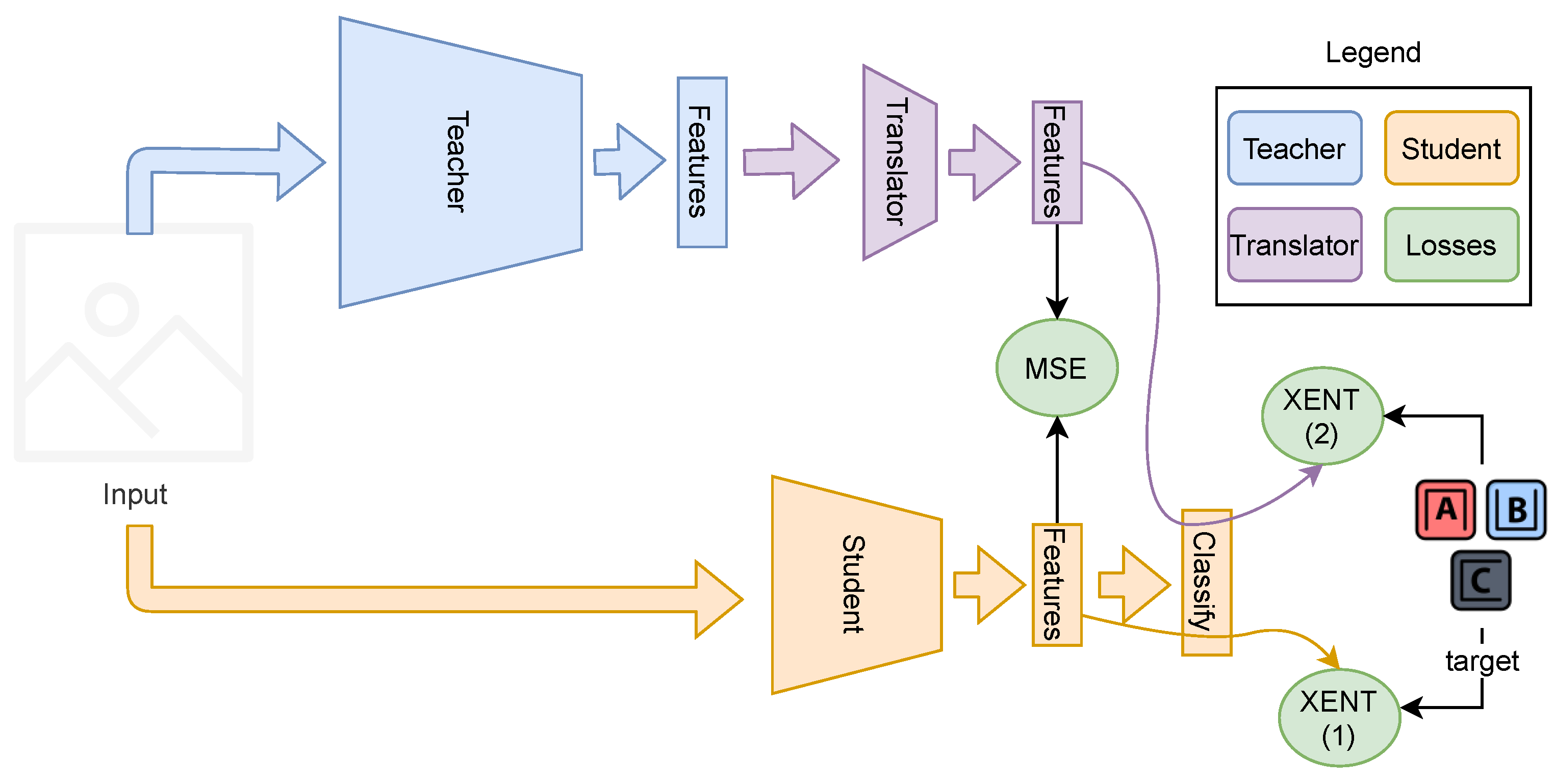
Since we experimentally discovered that, by eliminating the translator and inserting the whole transfer learning process within a single cycle, we were able to eliminate the problem highlighted in the Romero model, we can thus try to put the translator back, but this time, by adding a new loss function which in Figure 2 is called Xent (2). We do this to ensure that the translated features are, this time, as a function of the classification problem and not independently of this. Formally, the new cross-entropy loss introduced is defined in Equation (3) where we can see that the input values cl (fs) directly link the student’s features to the classification layer.
Compared to the solution analyzed in the previous section, we want to remove the limitation that the student and the teacher must have a layer with the same dimensions, but this time adding a new loss function. Thanks to the elimination of this constraint, in our proposed model, all types of networks, i.e., teachers, can teach any other type of network, i.e., students. In particular, we propose a translator layer plus a cross-entropy loss function to overcome this limitation. The translator can be represented by a simple layer or even by another network that transforms the dimensions of the teacher’s features layer into the dimensions of the student’s features layer, as we can see in Figure 2.
More formally, the cross-entropy loss indicates how far the model predictions are from the supervised labels (). The cross-entropy loss is defined as
which computes the loss between predicted classes’ probabilities x (in Figure 2, x is the output of the layer called Classify) and target y (in Figure 2, y is the target). In the training process, we update the model weights at each batch of size m. In Equation (1), n is the number of classes, so is the probability of the j-th class of the i-th prediction and is the probability corresponding to the -th class of the i-th prediction.
The MSE loss is used to minimize the distance between the teacher’s features and the student’s features. The general formula of this last loss function is defined as follows:
where is the student’s features ( is the name of the features layer) while is the teacher’s features.
Combining together the two losses defined in Equations (1) and (2), we obtain the loss proposed for our model. For the case where only one teacher is used, the loss function is the following:
where is the student’s features for layer , is the teacher’s features, and is the classification layer associated with the last layer of our model.
3.3. More Than One Teacher
From what we saw above with the introduction of our solution, we realized that it is always possible to take advantage of a single teacher. Now, we ask ourselves whether it is possible to generalize this concept to more teachers and understand under what conditions the introduction of other teachers in the transfer learning process continues to bring advantages. In the multi-teacher scenario, the final loss function uses the student’s last layers that are closest to the output layer or the classification layer. In particular, the teacher will use the layer , the teacher will use the layer , etc. As we did in the case of a single teacher in which we take their features layer and transfer it to the student through the use of the MSE loss with the student’s layer , generalizing this process for each teacher , we transfer their knowledge to the student via a new MSE loss between the features’ layer and the student layer (see Equation (5) for details). In addition to minimizing the distance between the features’ layers through the use of an MSE loss, as we did in our proposal in the case of a single teacher, we need a new additional (defined in Equation (1)) for each new teacher introduced. As shown in Figure 3, the features layer of teacher 2, called , is the same size as the student’s layer but not necessarily the same size as the student’s layer . This observation forces us to transform the size of into the size of before we can calculate the XENT3 loss shown in Figure 3. To perform this last step, the existing layer is used so the input values will be . This is best described in Equation (4). All this reasoning can be generalized to the case of a student with T teachers, as better described in Equation (5).
Below, we formalize the loss function in the case in which we only have two teachers:
where and are the translated features of the two teachers, are the student features into which we want to transfer the learning of the teachers, it the last layer function or classification layer, and y is the labels.
We can generalize the formula in Equation (4) for T-teachers using the function composition ∘ as . Consequently, the loss function of our model in the case where exactly T teachers and one student are used is the following:
Algorithm 1 describes the proposed approach that uses more than one teacher in a more formal way.
| Algorithm 1 Training step with more than one teacher |
| Input: |
| : the batched data |
| : the number of teachers |
| : the translator for teacher i |
| : the feature layers of the student |
| : the student model before the features layer of the transfer |
| : the teacher models |
|
3.4. Implementation Details
To implement our solution in an efficient way, we used back-propagation with the sum of all losses, but a different optimizer for each component: an optimizer for the translators and one for the student. In our situation, we used the same parameters so it is not fundamental, but it opens up the possibility of changing parameter for each optimizer.
To reduce memory usage, we can store the teacher’s features on file and customize the data loader to obtain the features for each teacher associated with the input and output data. This way, the teacher is not included in the learning process and therefore reduces the complexity of the model. To evaluate and compare the results, we used the following accuracy measure:
where is the number of samples correctly predicted by the model on whole test set and is the number of mistakes made by the model, so represents the total number of samples available in the test set.
3.5. Data Augmentation
To further improve the student’s generalization ability, we introduced a data augmentation strategy in the student network training process. In practice, we use a generic random generator able to represent a sequence of real numbers to build a two-dimensional array or image with random pixel values in the range of . We used these generated random images for each batch size as where N is a chosen integer that represents the number of random images to be created. In this way, for each training batch, a fixed number of randomly generated images were used by the teacher network to obtain the predicted label from it and were thus used to improve the student’s generalization ability.
This solution represents a simple technique for augmenting data in the case of problems with a low number of classes. It is not recommended that this technique is used for problems with many classes.
4. Datasets
In this work, we used five image datasets to conduct the various experiments. We moved from less complex datasets such as Cifar10 to very complex datasets such as ImageNet. Below, we briefly describe the datasets used.
Cifar10 [12] dataset consists of 60,000 images divided into 10 classes (6000 per class) with a training size and test size of 50,000 and 10,000, respectively. Each input sample is a color image with low resolution. The 10 classes are namely airplanes, cars, birds, cats, deer, dogs, frogs, horses, ships, and trucks.
Cifar100 [12] dataset consists of 60,000 images divided in 100 classes (600 per class) with a training size and test size of 50,000 and 10,000, respectively. Each input sample is a color images with low resolution.
In Figure 4, some representative examples of the two datasets are shown, extracted from a subset of classes.
This dataset is a good dataset because they are very useful in many papers. However, we also wanted to test it with a more real and difficult dataset. Thus, we merged the Stanford Dogs [13,14] dataset with the dogs species inside Oxford Cats and Dogs [15]. This merged dogs dataset (SOD) contained 131 classes and was used with a fixed split to obtain 20,492 training images and 5066 test images.
Cub200 2011 [16] is a dataset that we use to face up the fine-grained classification problem (Figure 5). It contains images of 200 species of birds split into 5994 and 5794 images for training and testing, respectively. Each image contains 15 part locations, 312 binary attributes, and 1 bounding boxes containing the bird within the image; however, we only used input images and their labels.
ImageNet is the most widely used dataset for image classification. This is mainly due to the high number of classes and the inhomogeneous collection images. We conducted an experiment using the ILSVRC2012 [17] version of this dataset, containing 1000 classes and 1.2 million images (see Figure 4). We used this dataset to obtain pre-trained models.
5. Experiments
In this section, we describe the set of conducted experiments. In particular, we conducted the following groups of experiments:
- In a first group of experiments, we want to understand whether the hypotheses of the problems found in the Romero model can be overcome;
- The second group of experiments serves to evaluate our proposed solution in which we add the translator linked to the new loss function;
- A last group of experiments aims to evaluate the introduction of more than one teacher for a single student.
In general, in all the experiments, we used Adam Optimizer and the Cosine Annealing learning rate function and performed a total of 200 training epochs.
5.1. Hypothesis Validation
In this first group of experiments summarized in Table 1 and Table 2, as described in Section 3.1, we eliminated the translator and changed the shape of the penultimate layer of the student to adapt it to the size of the features’ layer of the teacher. To try to understand how this solution works, we used different neural network models on the Cifa10, Cifar100, and Cub200 datasets. Furthermore, we compared the results with the original approaches proposed in Romero et al. [2] and KD [1].
For the experiment on Cifar10 and Cifar100, the size of the input images was set to and we also set a learning rate to , the batch size was set at 128, and we performed a total of 200 training epochs. We can see in Table 1 the comparison with the KD and Romero et al. approaches. We can see how the KD approach (which does not use the translator for features but uses the original values) works well compared to the Romero et al. approach which uses a translator. Our solution, on the other hand, without the translator, is able to outperform any other proposed method. The effectiveness of the data augmentation solution (see Section 3.5) on Cifar10, which has a limited number of classes, is particularly noteworthy. Instead, this method is less effective on Cifar100, which has a much higher number of classes. Table 1 validates our hypothesis at the translator level: the model proposed by Romero et al. without the translator level generally works better.
In this last experiment of this first group, we used the same dimensions of the features as for the previous experiments and the aim was to validate the goodness of our model. Table 2 reports all numerical results. We trained a MobileNetV2 [18] on the CUB200 dataset using a pre-trained model NTS-Net [8,19] as a teacher. The MobileNetV2 student feature layer was adapted to the size of the teacher that is 10240. We used a batch size equal to 10. In these experiments, we used size input images obtained by scaling the original image to and extracting a centered crop of size . In terms of the best results, the teacher-less experiments had a learning rate of which did not change over the epochs. Instead, for the experiment with the teacher, we have a learning rate of and after 100 epochs, it is multiplied by . In Table 2, we can see the accuracy of the student when trained without a teacher compared to the version trained using a teacher. We highlight the capability to increase the learning process using the same baseline but without the teacher model.
The NTS-Net [8] is a CNN successfully applied to solve fine-grained classification problems. This concatenates the features extracted from the whole image and four crops using attention mechanisms. We experimentally proved the effectiveness of our proposal over the CUB200 dataset and report the results in Table 2, where the student network can improve their accuracy thanks to teacher–student learning strategy.
5.2. Analysis of the Proposed Method with a Single Teacher and Student
As we saw in the previous group of experts, the problem is not the translator itself, but that the feature translation phase does not know that the features need to be translated for a classification problem that the student has to solve. From this observation, we introduced our proposal: the student topology is not modified and we introduced the translator again but this time, adding another cross-entropy loss function integrated with the transfer learning process. In this way, the student can learn from the teacher’s features while also learning to classify.
In this group of experiments, we used the Lenet5 and Mobilenetv3 models as students and Resnet50 and InceptionV3 as teachers on Cifar10 and Cifar100. The solution with only one teacher and one student proposed by us is compared with the accuracy reported by the model proposed by Romero et al. and by the KD model. In this group of experiments, the student model has the feature layer not adapted to the teacher size, because we have the translator. As in the other experiments on Cifar10 and Cifar100, the size of the input images was set to and we also set a learning rate to , the batch size was set at 128, and we performed a total of 200 training epochs. The results are reported in Table 3.
From the comparative results, we can see that the KD model, as we explained in Section 2 and as the authors demonstrated in their article [1], does not always show improvements in accuracy compared to the same model without transfer learning (in fact, their best result is obtained when they do the transfer learning between an ensemble and a single network, unlike what we do).
The approach proposed by Romero et al. gives good results in transferring learning between a complex network and a simplified version of the same network, but in a more generic case such as those shown in Table 3, we can see that its results are not exciting.
In conclusion, this group of experiments with Cifar10 and Cifar100, comparing our results with those of the other models, we can see that our proposal always improves accuracy using a single teacher and is therefore more reliable than the other solutions used.
5.3. Analysis of the Proposed Solution Using More Than One Teacher
Sometimes, the use of a second teacher can improve accuracy because the two teachers are trained on the same dataset but are two different types of networks. All the experts of this last group are reported in two tables. In Table 4, we analyze the behavior of our proposed model that uses more teachers, while in Table 5, we again analyze the model that uses more teachers but this time we want to understand whether the student is able to overcome one of the teachers thanks to transfer learning.
The experiments were conducted on two different datasets, and in particular, we chose to work on the SOD dataset (the results of which were reported in Table 4) and on the Cifar10 dataset (see results in Table 5) using a student with multiple parameters. In all of these experiments, however, we evaluate the version of our proposed model that uses two teachers.
Analyzing the data reported in the last line of Table 5, obtained on Cifar10, we can say that the student can exceed the performance of the teacher and of itself. In the experiment with two teachers, we use an Upsample layer instead of a linear layer related to the transfer between NTS-Net and Inceptionv3 as memory optimization.
However, to better understand the behavior of the proposed model that uses two teachers for the same student, in addition to analyzing the final accuracies reported in Table 4, we can see the behavior of the model during the entire training phase as shown in Figure 6. In this case, the student who uses two different teachers obtains the best results. We highlight in Figure 6 that the MobileNetv3 with two teacher approaches overcomes the others (orange and green lines). In this experiment, the student improves thanks to the contribution of two different teachers pretrained over the same dataset. Into the last row of Table 4, we used the same models demonstrating that two teachers pretrained over different datasets are more effective for the learning student process reporting an improvement in terms of accuracy.
In this last case, we have two different teachers, and in particular, we have an NTS-NET [8] which is a model for fine-grained classification and a ResNet50 [21,22] which is a well-known classification model. Therefore, in this situation where the two teachers implement two different approaches to the classification problem, we obtain an improvement in the student’s accuracy. In particular, in the last row of Table 4, we can see that if teachers are also trained on different datasets, then better results are obtained.
In the experiments of Table 4, we use a student who is smaller than the teacher in terms of the number of parameters, and therefore the results obtained by the student after transfer learning are never superior to those of the teacher. Thus, let us try on Cifar10 to replicate the experiment, this time using Inceptionv3 as a student and Resnet50 as a teacher. Resnet50 was also trained on ImageNet instead of using Cifar10 and NTS-Net was trained on SOD. As we can see in Table 5, both versions of ResNet50 used as teacher allow the student Inceptionv3 to overcome the results obtained by the teacher alone.
We can conclude this last group of experiments by saying that the best results with the single teacher were obtained when the teacher was trained on the same dataset. With two teachers on different datasets, students are also able to outperform the single teacher, the only student, and the single teacher on ImageNet.
6. Conclusions
Generally, the transfer learning technique is used as a fine-tuning technique to continue the training phase by using the weights learned on a huge dataset in order to achieve better and faster convergence performance. However, a transfer learning technique requires having the same model. In this work, we designed an efficient transfer learning methodology to train a student model from one or more than one pretrained different models without the need to have the same architectures. We confirm that a weak network (student) can learn more using a teacher. If we have two teachers with different skills (in terms of models and datasets), then the student is able to better improve its performance by using two teachers rather than just one. According to “The Lottery Ticket Hypothesis” [23], a smaller network can be equal to a larger one by pruning. Thus, using this hypothesis, we can apply our proposal in the future to find the best pruned network. Our proposal can transfer the learning from any networks so it is possible to test the transfer between a teacher trained on text classification to a student on image classification. In conclusion, we propose a new methodology to transfer learning from different models in a different way from the classical transfer learning techniques, demonstrating the effectiveness of our proposed approach on many different combinations of models and datasets.
Author Contributions
Conceptualization, N.L.; Supervision, I.G.; Validation, R.L.G. All authors have read and agreed to the published version of the manuscript.
Funding
This research received no external funding.
Institutional Review Board Statement
Not applicable.
Informed Consent Statement
Not applicable.
Data Availability Statement
Datasets used in this paper are in the public domain and can be found in the following links: CIFAR https://www.cs.toronto.edu/~kriz/cifar.html; Stanford Dogs http://vision.stanford.edu/aditya86/ImageNetDogs/; Oxford Cat and Dog https://www.kaggle.com/zippyz/cats-and-dogs-breeds-classification-oxford-dataset/; ImageNet https://www.image-net.org/; CUB200 http://www.vision.caltech.edu/visipedia/CUB-200.html.
Conflicts of Interest
The authors declare no conflict of interest.
References
- Hinton, G.; Vinyals, O.; Dean, J. Distilling the Knowledge in a Neural Network. arXiv 2015, arXiv:1503.02531. [Google Scholar]
- Romero, A.; Ballas, N.; Kahou, S.E.; Chassang, A.; Gatta, C.; Bengio, Y. FitNets: Hints for Thin Deep Nets. In Proceedings of the 3rd International Conference on Learning Representations, ICLR, San Diego, CA, USA, 7–9 May 2015. [Google Scholar]
- Ahn, S.; Hu, S.X.; Damianou, A.; Lawrence, N.D.; Dai, Z. Variational information distillation for knowledge transfer. In Proceedings of the IEEE Conference on Computer Vision and Pattern Recognition, Long Beach, CA, USA, 15–20 June 2019; pp. 9163–9171. [Google Scholar]
- Tung, F.; Mori, G. Similarity-preserving knowledge distillation. In Proceedings of the IEEE International Conference on Computer Vision, Seoul, Korea, 23 July 2019; pp. 1365–1374. Available online: https://openaccess.thecvf.com/content_ICCV_2019/papers/Tung_Similarity-Preserving_Knowledge_Distillation_ICCV_2019_paper.pdf (accessed on 11 November 2021).
- Srinivas, S.; Fleuret, F. Knowledge transfer with jacobian matching. arXiv 2018, arXiv:1803.00443. [Google Scholar]
- Lee, S.H.; Kim, D.H.; Song, B.C. Self-supervised knowledge distillation using singular value decomposition. In Proceedings of the European Conference on Computer Vision, Munich, Germany, 8–14 September 2018; pp. 339–354. [Google Scholar]
- Kornblith, S.; Shlens, J.; Le, Q.V. Do better imagenet models transfer better? In Proceedings of the IEEE/CVF Conference on Computer Vision and Pattern Recognition, Long Beach, CA, USA, 16–20 June 2019; pp. 2661–2671. [Google Scholar]
- Yang, Z.; Luo, T.; Wang, D.; Hu, Z.; Gao, J.; Wang, L. Learning to navigate for fine-grained classification. In Proceedings of the European Conference on Computer Vision (ECCV), Munich, Germany, 8–14 September 2018; pp. 420–435. [Google Scholar]
- Agarwal, N.; Sondhi, A.; Chopra, K.; Singh, G. Transfer learning: Survey and classification. In Smart Innovations in Communication and Computational Sciences; Springer: Berlin/Heidelberg, Germany, 2021; pp. 145–155. [Google Scholar]
- Goodfellow, I.J.; Warde-Farley, D.; Mirza, M.; Courville, A.; Bengio, Y. Maxout networks. arXiv 2013, arXiv:1302.4389. [Google Scholar]
- Landro, N. Features Transfer Learning. Available online: https://gitlab.com/nicolalandro/features_transfer_learning (accessed on 11 November 2021).
- Krizhevsky, A.; Hinton, G. Learning Multiple Layers of Features from Tiny Images; University of Toronto: Toronto, ON, Canada, 2009; Available online: http://citeseerx.ist.psu.edu/viewdoc/download?doi=10.1.1.222.9220&rep=rep1&type=pdf (accessed on 11 November 2021).
- Khosla, A.; Jayadevaprakash, N.; Yao, B.; Fei-Fei, L. Novel Dataset for Fine-Grained Image Categorization. In Proceedings of the First Workshop on Fine-Grained Visual Categorization, Colorado Springs, CO, USA, 20–25 June 2011; Available online: https://people.csail.mit.edu/khosla/papers/fgvc2011.pdf (accessed on 11 November 2021).
- Deng, J.; Dong, W.; Socher, R.; Li, L.J.; Li, K.; Fei-Fei, L. ImageNet: A Large-Scale Hierarchical Image Database. In Proceedings of the 2009 IEEE Conference on Computer Vision and Pattern Recognition, Miami, FL, USA, 20–25 June 2009. [Google Scholar]
- Parkhi, O.M.; Vedaldi, A.; Zisserman, A.; Jawahar, C. Cats and dogs. In Proceedings of the 2012 IEEE Conference on Computer Vision and Pattern Recognition, Providence, RI, USA, 16–21 June 2012; pp. 3498–3505. [Google Scholar]
- Wah, C.; Branson, S.; Welinder, P.; Perona, P.; Belongie, S. The Caltech-UCSD Birds-200-2011 Dataset; Technical Report CNS-TR-2011-001; California Institute of Technology: Pasadena, CA, USA, 2011. [Google Scholar]
- Russakovsky, O.; Deng, J.; Su, H.; Krause, J.; Satheesh, S.; Ma, S.; Huang, Z.; Karpathy, A.; Khosla, A.; Bernstein, M.; et al. ImageNet Large Scale Visual Recognition Challenge. Int. J. Comput. Vis. (IJCV) 2015, 115, 211–252. [Google Scholar] [CrossRef] [Green Version]
- Sandler, M.; Howard, A.; Zhu, M.; Zhmoginov, A.; Chen, L.C. Mobilenetv2: Inverted residuals and linear bottlenecks. In Proceedings of the IEEE Conference on Computer Vision and Pattern Recognition, Salt Lake City, UT, USA, 18–23 June 2018; pp. 4510–4520. [Google Scholar]
- Nawaz, S.; Calefati, A.; Caraffini, M.; Landro, N.; Gallo, I. Are These Birds Similar: Learning Branched Networks for Fine-grained Representations. In Proceedings of the 2019 International Conference on Image and Vision Computing New Zealand (IVCNZ), Dunedin, New Zealand, 2–4 December 2019; pp. 1–5. [Google Scholar]
- Landro, N. 131 Dog’s Species Classification. Available online: https://github.com/nicolalandro/dogs_species_prediction (accessed on 11 November 2021).
- He, K.; Zhang, X.; Ren, S.; Sun, J. Deep Residual Learning for Image Recognition. arXiv 2015, arXiv:1512.03385. [Google Scholar]
- Targ, S.; Almeida, D.; Lyman, K. Resnet in resnet: Generalizing residual architectures. arXiv 2016, arXiv:1603.08029. [Google Scholar]
- Frankle, J.; Carbin, M. The lottery ticket hypothesis: Finding sparse, trainable neural networks. arXiv 2018, arXiv:1803.03635. [Google Scholar]
Figure 1.
Intuitive representation of the proposed approach: a neural network called student, represented as a small robot, can directly learn from the original data represented on the blackboard and also from the knowledge acquired by more than one teacher. The light on the teachers’ head, unlike the student’s, is not on because their learning is blocked.

Figure 2.
Proposed approach with one teacher. We can distinguish three different networks: the teacher, the translator, and the student. The loss function is composed by the mean squared error (MSE) between the student and translator plus the first cross-entropy (XENT (1)) of the student’s feature and classify layer flow, plus the second cross-entropy (XENT (2)) of the translator’s feature and classify layer flow.

Figure 3.
Proposed approach with two teachers. We can distinguish four different networks: the teacher, the translator 1, the translator 2, and the student. The loss functions MSE(1), XENT(1), and XENT(2) are composed as in Figure 2, however, here we also add MSE(2) between the features of Translator2 and the student’s layer Features2 and the third cross-entropy XENT(3) using the features of Translator2 and the student’s classification layer.

Figure 4.
On the left are some sample images for each of the 10 classes of CIFAR-10 (one class for each row). On the right are 10 randomly selected classes from the set of 100 classes of CIFAR-100.
Figure 4.
On the left are some sample images for each of the 10 classes of CIFAR-10 (one class for each row). On the right are 10 randomly selected classes from the set of 100 classes of CIFAR-100.

Figure 5.
A sample image for each of the 200 classes of the CUB200-2011 dataset.

Figure 6.
Test accuracy over the SOD dataset. The student network is a MobileNetv3. The teacher one is an NTS-NET. Teacher two is the ResNet50.
Figure 6.
Test accuracy over the SOD dataset. The student network is a MobileNetv3. The teacher one is an NTS-NET. Teacher two is the ResNet50.


Table 1.
Comparison of the baseline test accuracies on the Cifar10 and Cifar100 datasets with the knowledge distillation (KD) [1], Romero approach [2], with one teacher (T1S) and one teacher with augmentation (T1S + Aug.), after 200 epochs, using two Resnet50 as teachers (one for Cifar10 and one for Cifar100). The student is of the same size as the feature layer adapted to that of the teacher.
| Name | Baseline | KD | Romero | T1S | T1S + Aug. |
|---|---|---|---|---|---|
| Cifar10 | |||||
| Lenet5 | 65.43 | 64.84 | 62.11 | 64.12 | 65.49 |
| AlexNet | 72.75 | 70.93 | 70.38 | 73.74 | 73.99 |
| MobileNetV2 | 74.82 | 63.22 | 64.92 | 77.53 | 81.60 |
| Resnet18 | 78.76 | 82.64 | 82.35 | 80.81 | 83.52 |
| Cifar100 | |||||
| Lenet5 | 28.34 | 32.62 | 29.72 | 33.86 | 33.65 |
| AlexNet | 35.86 | 36.93 | 37.96 | 40.49 | 38.12 |
| MobileNetV2 | 31.31 | 29.03 | 31.26 | 43.25 | 39.47 |
| Resnet18 | 51.82 | 46.42 | 46.03 | 60.77 | 54.18 |
Table 2.
In this table, we report the test accuracy obtained by a MobileNetV2 used as a student with an NTS-Net as a teacher over CUB200 dataset.
Table 2.
In this table, we report the test accuracy obtained by a MobileNetV2 used as a student with an NTS-Net as a teacher over CUB200 dataset.
| Name | Without Teacher | With Teacher |
|---|---|---|
| MobileNetV2 | 42.5 | 49.2 |
Table 3.
Accuracy in percentage after 200 epochs over Cifar10 and Cifar100 using InceptionV3 (T1) and T1 plus Resnet50 (T2) as teachers. The baseline here is the model that does not have the modified layer because we make use of the translator.
Table 3.
Accuracy in percentage after 200 epochs over Cifar10 and Cifar100 using InceptionV3 (T1) and T1 plus Resnet50 (T2) as teachers. The baseline here is the model that does not have the modified layer because we make use of the translator.
| Dataset | Student | Baseline | Romero | KD | T1 | T2 |
|---|---|---|---|---|---|---|
| Cifar10 | Lenet5 | 64.12 | 60.64 | 61.01 | 64.77 | 64.89 |
| Cifar10 | Mobilenetv3 | 60.98 | 62.12 | 60.59 | 64.42 | 64.29 |
| Cifar100 | Lenet5 | 32.60 | 32.37 | 33.57 | 34.25 | 34.09 |
| Cifar100 | Mobilenetv3 | 30.26 | 30.29 | 25.22 | 31.78 | 33.17 |
Table 4.
We report the results after 200 epochs of a MobileNetV3 with a classical teacher and with a fine-grained teacher such as NTS-NET (demo available in [20]) on SOD datasets.
Table 4.
We report the results after 200 epochs of a MobileNetV3 with a classical teacher and with a fine-grained teacher such as NTS-NET (demo available in [20]) on SOD datasets.
| Student | Teacher/s | Pretrained | Accuracy |
|---|---|---|---|
| MobileNetV3 | - | - | 49.59 |
| MobileNetV3 | Resnet50 | SOD | 53.00 |
| MobileNetV3 | Resnet50, Nts-Net | SOD, SOD | 55.53 |
| MobileNetV3 | Resnet50, Nts-Net | ImageNet, SOD | 57.15 |
Table 5.
In this Table, we report the results using an InceptionV3 model on Cifar10 with a Resnet50 teacher model trained on ImageNet or trained on Cifar10 (200 epochs).
Table 5.
In this Table, we report the results using an InceptionV3 model on Cifar10 with a Resnet50 teacher model trained on ImageNet or trained on Cifar10 (200 epochs).
| Student | Teacher/s | Teacher Train | Student Train | Accuracy |
|---|---|---|---|---|
| - | Resnet50 | Cifar10 | - | 82.39 |
| Inceptionv3 | - | - | Cifar10 | 72.81 |
| Inceptionv3 | Resnet50 | ImageNet | Cifar10 | 91.39 |
| Inceptionv3 | Resnet50, Nts-Net | ImageNet, SOD | Cifar10 | 92.00 |
| Inceptionv3 | Resnet50 | Cifar10 | Cifar10 | 92.10 |
Publisher’s Note: MDPI stays neutral with regard to jurisdictional claims in published maps and institutional affiliations. |
© 2021 by the authors. Licensee MDPI, Basel, Switzerland. This article is an open access article distributed under the terms and conditions of the Creative Commons Attribution (CC BY) license (https://creativecommons.org/licenses/by/4.0/).
Share and Cite
MDPI and ACS Style
Landro, N.; Gallo, I.; La Grassa, R. Is One Teacher Model Enough to Transfer Knowledge to a Student Model? Algorithms 2021, 14, 334. https://0-doi-org.brum.beds.ac.uk/10.3390/a14110334
AMA Style
Landro N, Gallo I, La Grassa R. Is One Teacher Model Enough to Transfer Knowledge to a Student Model? Algorithms. 2021; 14(11):334. https://0-doi-org.brum.beds.ac.uk/10.3390/a14110334
Chicago/Turabian StyleLandro, Nicola, Ignazio Gallo, and Riccardo La Grassa. 2021. "Is One Teacher Model Enough to Transfer Knowledge to a Student Model?" Algorithms 14, no. 11: 334. https://0-doi-org.brum.beds.ac.uk/10.3390/a14110334
Note that from the first issue of 2016, this journal uses article numbers instead of page numbers. See further details here.