
Representing Deep Neural Networks Latent Space Geometries with Graphs


1
Electronics Department, IMT Atlantique, 29280 Brest, France
2
Department of Electrical and Computer Engineering, University of Southern California, Los Angeles, CA 90007, USA
*
Author to whom correspondence should be addressed.
Algorithms 2021, 14(2), 39; https://0-doi-org.brum.beds.ac.uk/10.3390/a14020039
Submission received: 13 November 2020
/
Revised: 14 January 2021
/
Accepted: 19 January 2021
/
Published: 27 January 2021
(This article belongs to the Special Issue Efficient Graph Algorithms in Machine Learning)
Abstract
:Deep Learning (DL) has attracted a lot of attention for its ability to reach state-of-the-art performance in many machine learning tasks. The core principle of DL methods consists of training composite architectures in an end-to-end fashion, where inputs are associated with outputs trained to optimize an objective function. Because of their compositional nature, DL architectures naturally exhibit several intermediate representations of the inputs, which belong to so-called latent spaces. When treated individually, these intermediate representations are most of the time unconstrained during the learning process, as it is unclear which properties should be favored. However, when processing a batch of inputs concurrently, the corresponding set of intermediate representations exhibit relations (what we call a geometry) on which desired properties can be sought. In this work, we show that it is possible to introduce constraints on these latent geometries to address various problems. In more detail, we propose to represent geometries by constructing similarity graphs from the intermediate representations obtained when processing a batch of inputs. By constraining these Latent Geometry Graphs (LGGs), we address the three following problems: (i) reproducing the behavior of a teacher architecture is achieved by mimicking its geometry, (ii) designing efficient embeddings for classification is achieved by targeting specific geometries, and (iii) robustness to deviations on inputs is achieved via enforcing smooth variation of geometry between consecutive latent spaces. Using standard vision benchmarks, we demonstrate the ability of the proposed geometry-based methods in solving the considered problems.
1. Introduction
In recent years, Deep Learning (DL) methods have achieved state of the art performance in a vast range of machine learning tasks, including image classification [1] and multilingual automatic text translation [2]. A DL architecture is built by assembling elementary operators called layers [3], some of which contain trainable parameters. Due to their compositional nature, DL architectures exhibit intermediate representations when they process a given input. These intermediate representations lie in so-called latent spaces.
DL architectures are typically trained to minimize a loss function computed at their output. This is performed using a variant of the stochastic gradient descent algorithm that is backpropagated through the multiple layers to update the corresponding parameters. To accelerate the training procedure, it is very common to process batches of inputs concurrently. In such a case, a global criterion over the corresponding batch (e.g., the average loss) is backpropagated.
The training procedure of DL architectures is thus performed in an end-to-end fashion. This end-to-end characteristic of DL refers to the fact that intermediate representations are unconstrained during training. This property has often been considered as an asset in the literature [4] which presents DL as a way to replace “hand-crafted” features by automatic differentiation. As a matter of fact, using these hand-crafted features as intermediate representations can cause sub-optimal solutions [5]. On the other hand, completely removing all constraints on the intermediate representations can cause the learning procedure to exhibit unwanted behavior, such as susceptibility to deviations of the inputs [6,7,8], or redundant features [9,10].
In this work, we propose a new methodology aiming at enforcing desirable properties on intermediate representations. Since training is organized into batches, we achieve this goal by constraining what we call the latent geometry of data points within a batch. This geometry refers to the relative position of data points within a specific batch, based on their representation in a given layer. While there are many problems for which specific intermediate layer properties are beneficial, in this work, we consider three examples. First, we explore compression via knowledge distillation (KD) [9,10,11,12], where the goal is to supervise the training procedure of a small DL architecture (called the student) with a larger one (called the teacher). Second, we study the design of efficient embeddings for classification [13,14], in which the aim is to train the DL architecture to be able to extract features that are useful for classification (and could be used by different classifier) rather than using classification accuracy as the sole performance metric. Finally, we develop techniques to increase the robustness of DL architectures to deviations of their inputs [6,7,8].
To address the three above-mentioned problems, we introduce a common methodology that exploits the latent geometries of a DL architecture. More precisely, we propose to formalize latent geometries by defining similarity graphs. In these graphs, vertices are data points in a batch and an edge weight between two vertices is a function of the relative similarity between the corresponding intermediate representations at a given layer. We call such a graph a latent geometry graph (LGG). In this paper, we show that intermediate representations with desirable properties can be obtained by imposing constraints on their corresponding LGGs. In the context of KD, similarity between teacher and student is favored by minimizing the discrepancy between their respective LGGs. For efficient embedding designs, we propose a LGG-based objective function that favors disentanglement of the classes. Lastly, to improve robustness, we enforce smooth variations between LGGs corresponding to pairs of consecutive layers at any stage, from input to output, in a given architecture. Enforcing smooth variations between the LGGs of consecutive layers provides some protection against noisy inputs, since small changes in the input are less likely to lead to a sharp transition of the network’s decision.
This paper is structured as follows; we first discuss related work in Section 2. We then introduce the proposed methodology in Section 3. Then, we present the three applications, namely knowledge distillation, design of classification feature vectors, and robustness improvements, in Section 4. Finally, we present a summary and a discussion on future work in Section 5. A term glossary is available in Appendix A.
2. Related Work
As previously mentioned, in this work, we are interested in using graphs to ensure that latent spaces of DL architectures have some desirable properties. The various approaches we introduce in this paper are based on our previous contributions [8,10,14]. However, in this paper, they are presented for the first time using a unified methodology and formalism. While we deployed these ideas already in a few applications, by presenting them in a unified form, our goal is to provide a broader perspective of these tools, as well as to encourage their use for other problems.
In what follows, we introduce related work found in the literature. We start by comparing our approach with others that also aim at enforcing properties on latent spaces. Then, we discuss approaches that mix graphs and intermediate (or latent) representations in DL architectures. Finally, we discuss methods related to the applications highlighted in this work: (i) knowledge distillation, (ii) latent embeddings, and (iii) robustness.
Enforcing properties on latent spaces: A core goal of our work is to enforce desirable properties on the latent spaces of DL architectures, more precisely (i) consistency with a teacher network, (ii) class disentangling, and (iii) smooth variation of geometries over the architecture. In the literature, one can find two types of approaches to enforce properties on latent spaces: (i) directly designing specific modules or architectures [15,16] and (ii) modifying the training procedures [11,13]. The main advantage of the latter approaches is that one is able to draw from the vast literature in DL architecture design [17,18] and use an existing architecture instead of having to design a new one.
Our proposed unified methodology can be seen as an example of the second type of approaches, with two main advantages over competing techniques. First, by using relational information between the examples, instead of treating each one separately, we extend the range of proposed solutions. For example, relational knowledge distillation methods can be applied to any pair of teacher-student networks [9] as relational metrics are dependent on the number of examples and not on the dimension of individual layers (see more details in the next paragraphs). Second, by using graphs to represent the relational information, we are able to to exploit the rich literature in graph signal processing [19] and use it to reason about the properties we aim at enforcing on latent spaces. We discuss this in more detail in Section 4.1 and Section 4.3.
Latent space graphs: In the past few years, there has been a growing interest in proposing deep neural network layers able to process graph-based inputs, also known as graph neural networks. For example, works, such as References [20,21,22,23], show how one can use convolutions defined in graph domains to improve performance of DL methods dealing with graph signals as inputs. The proposed methodology differs from these works in that it does not require inputs to be defined on an explicit graph. The graphs we consider here (LGGs) are proxies to the latent data geometry of the intermediate representations. Contrary to classical graph neural networks, the purpose of the proposed methodology is to study latent representations using graphs, instead of processing graph supported inputs. Some recent work can be viewed as following ideas similar to those introduced in this paper, with applications in areas, such as knowledge distillation [24,25], robustness [15], interpretability [26], and generalization [27]. Despite sharing a common methodology, these works are not explicitly linked. This can be explained by the fact that they were introduced independently around the same time and have different aims. We provide more details about how they are connected with our proposed methodology in the following paragraphs.
Knowledge distillation: Knowledge distillation is a DL compression method, where the goal is to use the knowledge acquired on a pre-trained architecture, called teacher, to train a smaller one, called student. Initial works on knowledge distillation considered each input independently from the others, an approach known as Individual Knowledge Distillation (IKD) [11,12,28]. As such, the student architecture mimics the intermediate representations of the teacher for each input used for training. The main drawback of IKD lies in the fact that it forces intermediate representations of the student to be of the same dimensions of that of the teacher. To deploy IKD in broader contexts, authors have proposed to disregard some of these intermediate representations [12] or to perform some-kind of dimensionality reduction [28].
On the other hand, the method we propose in Section 4.1 is based on a recent paradigm named Relational Knowledge Distillation (RKD) [9], which differs from IKD as it focuses on the relationship between examples instead of their exact positions in latent spaces. RKD has the advantage of leading to dimension-agnostic methods, such as the one described in this work. By defining graphs, its main advantage lies in the fact relationships between elements are considered relatively to each other.
Concurrently, other authors [24,25] have proposed methods similar to the one we present here [10]. In Reference [24], unlike in our approach, dimensionality reduction transformations are added to the intermediate representations, in an attempt to improve the knowledge distillation. In Reference [25], LGGs are built using attention (similar to Reference [29]). Among other differences, we show in Section 4.1 that constructing graphs that only connect data points from distinct classes can significantly improve accuracy.
Latent embeddings: In the context of classification, the most common DL setting is to train the architecture end-to-end with an objective function that directly generates a decision at the output. Instead, it can be beneficial to output representations well suited to be processed by a simple classifier (e.g., logistic regression). This framework is called feature extraction or latent embeddings, as the goal is to generate representations that are easy to classify, but without directly enforcing the way they should be used for classification. Such a framework is very interesting if the DL architecture is not going to be used solely for classification but also for related tasks, such as person re-identification [13], transfer learning [30], and multi-task learning [31].
Many authors have proposed ways to train deep feature extractors. One influential example is Reference [13], where the authors use triplets to perform Deep Metric Learning. In each triplet, the first element is the example to train, the second is a positive example (e.g., same class) and the last is a negative one (e.g., different class). The aim is to result in triplets where the first element is closer to the second than to the last. In contrast, our method considers all connections between examples of different classes and can focus solely on separation (making all the negatives far) instead of clustering (making all the positives close), which we posit should lead to more robust embeddings in Section 4.2.
Other solutions for generating latent embeddings propose alternatives to the classical arg max operator used to perform the decision at the output of a DL architecture. This can be done either by changing the output so that it is based on error correcting codes [32] or is smoothed, either explicitly [33] or by using the prior knowledge of another network [11].
Robustness of DL architectures: In this work, we are interested in improving the robustness of DL architectures. We define robustness as the ability of the network to correctly classify inputs even if they are subject to small perturbations. These perturbations may be adversarial (designed exactly to force misclassification) [34] or incidental (due to external factors, such as hardware defects or weather artifacts) [7]. The method we present in Section 4.3 is able to increase the robustness of the architecture in both cases. Multiple works in the literature aim to improve the robustness of DL architectures following two main approaches: (i) training set augmentation [35] and (ii) improved training procedure. Our contribution can be seen as an example of the latter approaches, but can be combined with augmentation-based methods, leading to an increase of performance compared to using the techniques separately [8].
A similar idea was proposed in Reference [15], where the authors exploit graph convolutional layers in order to improve robustness of DL architectures applied to non-graph domains. Their approach can be described as denoising the (test) input by using the training data. This differs from the method we propose in Section 4.3, which focuses on generating a smooth network function. As such, the proposed method is more general as it is less dependent on the training set.
3. Methodology
In this section, we first introduce basic concepts from DL and graph signal processing (Section 3.1 and Section 3.2) and then our proposed methodology (Section 3.3).
3.1. Deep Learning
We start by introducing basic deep learning (DL) concepts, referring the reader to Reference [3] for a more in-depth overview. A DL architecture is an assembly of layers that can be mathematically described as a function f, often referred to as the “network function” in the literature, that associates an input tensor x with an output tensor . This function is characterized by a large number of trainable parameters . In the literature, many different approaches have been proposed to assemble layers to obtain such network functions [17]. While layers are the basic unit, it is also common to describe architectures in terms of a series of blocks, where a block is typically a small set of connected layers. This block representation allows us to encapsulate non-sequential behaviors, such as the residual connections of residual networks (Resnets) [17], so that, even though layers are connected in a more complex way, the blocks remain sequential, and the network function can be represented as a series of cascading operations:
where each function can represent a layer, or a block comprising several layers, depending on the underlying DL architecture. Thus, each block is associated with a subfunction . For example, in the context of Resnets [17], the architecture is composed of blocks as depicted in Figure 1.
A very important concept for the remainder of this work is that of intermediate representations, which are the basis for the LGGs (defined in Section 3.3) and corresponding applications (Section 4).
Definition 1
(Intermediate representation). We call intermediate representation of an input x the output it generates at an intermediate layer or block. Starting from Equation (1), and denoting we define the intermediate representation at depth ℓ for x as . Or, said otherwise, is the representation of in the latent space at depth ℓ.
Initially, the parameters of f are typically drawn at random. They are then optimized during the training phase so that f achieves a desirable performance for the problem under consideration. The dimension of the output of f depends on the task. In the context of classification, it is common to design the network function such that the output has a dimension equal to the number of classes in the classification problem. In this case, for a given input, each coordinate of this final layer output is used as an estimate of the likelihood that the input belongs to the corresponding class. A network function correctly maps an input to its class if the output of the network function, , is close to the target vector of the correct class y.
Definition 2
(Target vector). Each sample of the training set is associated with a target vector of dimension C, where C is the total number of classes. Thus, the target vector of a sample of class c is the binary vector containing 1 at coordinate c and 0 at all other coordinates.
In this work, we also introduce the notion of label indicator vector, which it is important to differentiate from that of target vector. The label indicator vector is defined on a batch of data points, instead of individually for each sample, as follows:
Definition 3
(Label indicator vector). Consider a batch of B data points. The label indicator vector of class c for this batch is the binary vector containing 1 at coordinate i if and only if the i-th element of the batch is of class c, and 0 otherwise.
The purpose of a classification problem is to obtain a network function f that outputs the correct class decision for any valid input x. In practice, it is often the case that the set of valid inputs is not finite, and yet we are only given a “small” number of pairs (x, y), where y is the output associated with x. The set of these pairs is called the dataset . During the training phase, the parameters are tuned using and an objective function that measures the discrepancy between the outputs of the network function and expected target indicator vectors, i.e., the discrepancy between and. It is common to decompose the function f into a feature extractor and a classifier as follows: . In a classification task, the objective function is calculated over the outputs of the classifier and the gradients are backpropagated to generate a good feature extractor. Alternatively, to ensure that good latent embeddings are produced, one can first optimize the feature extractor part of the architecture to optimize the features and then a classifier can be trained based on the resulting features (which remain fixed or not) [13,14]. We introduce an objective function designed for efficient latent embedding training in Section 4.2.
Usually, the objective function is a loss function. It is minimized over a subset of the dataset that we call “training set” (). The reason to select a subset of to train the DL architecture is that it is hard to predict the generalization ability of the trained function f. Generalization usually refers to the ability of f to predict the correct output for inputs x not in . A simple way to evaluate generalization consists of counting the proportion of elements in that are correctly classified using f. Obviously, this measure of generalization is not ideal, in the sense that it only checks generalization inside . This is why it is possible for a network that seems to generalize well to have trouble to classify inputs that are subject to deviations. In this case, it is said that the DL architecture is not robust. We delve into more details on robustness in Section 4.3
In summary, a network function is initialized at random. Parameters are then tuned using a variant of the stochastic gradient descent algorithm on a dataset , and finally, training performance is evaluated on a validation set. Problematically, the best performance of DL architectures strongly depends on the total number of parameters they contain [36]. In particular, it has been hypothesized that this dependence comes from the difficulty of finding a good gradient trajectory when the parameter space dimension is small [37]. A common way to circumvent this problem is to rely on knowledge distillation, where a network with a large number of parameters is used to supervise the training of a smaller one. We introduce a graph-based method for knowledge distillation in Section 4.1.
3.2. Graph Signal Processing
As mentioned in the introduction, graphs are ubiquitous objects to represent relationships (called edges) between elements in a countable set (called vertices). In this section, we introduce the framework of Graph Signal Processing (GSP) which is central to our proposed methodology. Let us first formally define graphs:
Definition 4
(graph). A graph is a tuple of sets , such that:
- 1.
- The finite set is composed of vertices .
- 2.
- The set is composed of pairs of vertices of the form (,) called edges.
It is common to represent the set using an edge-indicator symmetric adjacency matrix . Note that, in this work, we consider only undirected graphs corresponding to symmetric (i.e., ). In some cases, it is useful to consider (edge-)weighted graphs. In that case, the adjacency matrix can take values other than 0 or 1.
We can use to define the diagonal degree matrix D of the graph as:
In the context of GSP, we consider not only graphs but also graph signals. A graph signal is typically defined as a vector s. In this work, we often consider a set of signals jointly. We group the signals in a matrix , where each of the columns is an individual graph signal s. An important notion in the remaining of this work is that of graph signal variation.
Definition 5
(Graph signal variation). The total variation σ of a set of graph signals represented by S is:
where is the combinatorial Laplacian of the graph that supports S, and tr is the trace function. We can also rewrite σ as:
where represents the signal s defined on vertex . As such, the variation of a signal increases when vertices connected by edges with large weights have very different values.
3.3. Proposed Methodology
In this section, we describe how to construct and exploit latent geometry graphs (LGGs) and illustrate the key ideas with a toy example. Given a batch X, each LGG vertex corresponds to a sample in X, and each edge weight measures similarity between the corresponding data points. More specifically, LGGs are constructed as follows:
- (1)
- Generate a symmetric square matrix using a similarity measure between intermediate representations, at a given depth ℓ, of data points in X. In this work, we choose the cosine similarity when data is non-negative, and an RBF similarity kernel based on the L2 distance otherwise.
- (2)
- Threshold so that each vertex is connected only to its k-nearest neighbors.
- (3)
- Symmetrize the resulting thresholded matrix: two vertices i and j are connected with edge weights as long one of the nodes was a k nearest neighbor of the other.
- (4)
- (Optional) Normalize using its degree diagonal matrix: .
Given the LGG associated to some intermediate representation, we are able to quantify how well this representation matches the classification task under consideration by using the concept of label variation, a measure of graph signal variation for a signal formed as a concatenation of all label indicator vectors:
Definition 6
(Label variation). Consider a similarity graph for a given batch X (obtained from some intermediate layer), represented by an adjacency matrix , and define a label indicator matrix V obtained by concatenating label indicator vectors of each class. Label variation is defined as:
Remark 1.
Label variation has the advantage of being independent of the choice of labels for each class, which can be verified by noticing that for any permutation matrix P, it holds that:
If the graph is well suited for classification, then most nodes will have immediate neighbors in the same class. Indeed, label variation is 0 if and only if data points that belong to distinct classes are not connected in the graph. Therefore, smaller label variation is indicative of an easier classification task (well separated classes).
3.3.1. Toy Example
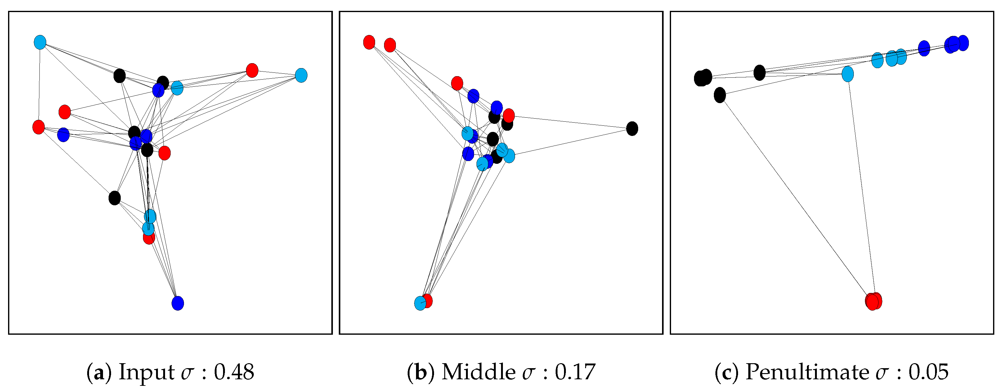
In this example, we visualize the relation between the classification task and the geometries represented by the graphs. To do so, we construct three similarity graphs for a very small subset (20 images from 4 classes are used, i.e., 5 images per class) of the CIFAR-10 (Appendix B) , one defined on the image space (i.e., computing the similarity between the 3072 dimensions of the raw input images) and two using the latent space representations of an architecture trained on the dataset. Such representations come from an intermediate layer (32,768 dimensions) and the penultimate layer (512 dimensions). What we expect to see qualitatively is that the classes will be easier to separate as we go deeper in the considered architecture, which should be reflected by the label variation score: the penultimate layer should yield the smallest label variation. We depict this example in Figure 2. Note that data points are placed in the 2D space using Laplacian eigenmaps [38]. As expected, we can qualitatively see the difference in separation from the image space to the latent spaces. We are also able to measure quantitatively how difficult it is to separate the classes using the label variation, which is lowest for the penultimate layer. For more details on how this example was generated, we refer the reader to Appendix C.
3.3.2. Dimensionality and LGGs
A key asset of the proposed methodology is that the number of vertices in the graph is independent of the dimension of the intermediate representations it was built from. As such, it is possible to compare graphs built from latent spaces with various dimensions, as illustrated in Figure 2. Being agnostic to dimension will be a key ingredient in the applications described in the following section. It is important to note that, while the number of vertices is independent of the dimension of intermediate representations, edge weights are a function of a similarity in the considered latent space, which can have very different meanings depending on the underlying dimensions.
In the context of DL architectures, a common choice of similarity measure is that of cosine. Interestingly, cosine similarity is well defined only for nonnegative data (as typically processed by a ReLU function) and bounded between 0 and 1. When data can be negative, we use a Gaussian kernel applied to the Euclidean distance instead. The problem remains that cosine or Euclidean similarities suffers from the curse of dimensionality. In an effort to reduce the influence of dimension when comparing LGGs obtained from latent spaces with distinct dimensions, in our experiments, we make use of graph normalization, as defined in step 4 of LGG construction. We also provide a discussion on the complexity of graph similarity computation in Appendix D. Note that a more in-depth analysis and understanding of the influence of dimension on graph construction is a promising direction for future work, as improving the graph construction could benefit all applications covered in this work.
4. Applications
We now show how LGGs can be used in three specific applications: (i) knowledge distillation, (ii) latent embeddings, and (iii) robustness. Details on the dataset used can be found in Appendix B.
4.1. Knowledge Distillation
First, we consider the case of knowledge distillation (KD). The goal of KD is to use the knowledge acquired by a pre-trained DL architecture that we call teacher T to train a second architecture called student S. KD is normally performed in compression scenarios where the goal is to obtain an architecture S that is less computationally expensive than T while maintaining good enough generalization. In order to do so, KD approaches aim at making both networks consistent in their decisions. Consistency is usually achieved by minimizing a measure of discrepancy between the networks intermediate and/or final representations.
More formally, we can define the objective function of the student networks trained with knowledge distillation as:
where is typically the same loss that was used to train the teacher (e.g., cross-entropy), is the distillation loss, and is a scaling parameter to control the importance of the distillation with respect to that of the task.
Recall that Individual Knowledge Distillation (IKD) requires intermediate representations of T and S to be of the same dimensions. In order to avoid this drawback, Relational Knowledge Distillation (RKD) has been recently proposed [9,24,25]. Indeed, the method we introduce in this section is inspired by Reference [9], where the authors propose to compare the distance obtained between the intermediate representations of a pair of data points in the teacher with the corresponding distance for the student. The goal then becomes to minimize the variation between these two distances. Interestingly, distances can be compared even if the corresponding intermediate representations do not have the same dimension. However, we point out that forcing (absolute) distances to be similar is not necessarily desirable. As a matter of fact, it would be sufficient to consider distances relatively to other pairs of data points. For example: consider a case where in the teacher latent space the distance between points A and B is 0.5, and the distance between points A and C is 0.25. Instead of forcing the student to have the same distances, as well (0.5 and 0.25), we could just ensure that the AC distance is half of the AB distance.
In this section, we introduce a method that focuses on distilling the learnt latent topologies that we represent by LGGs. This can be seen as distilling the relative distances between samples, differently from the previously presented RKD-D, which distills absolute distances. The framework we consider, that we named Graph Knowledge Distillation (GKD) in Reference [10], consists of reducing the discrepancy between LGGs constructed in T and S.
Proposed approach (GKD): Let us consider a layer in the teacher architecture, and the corresponding one in the student architecture. Considering a batch of inputs, we propose to build the corresponding graphs and capturing their geometries as described in Section 3.3.
During training, we propose to use the following loss in Equation (7):
where is the Frobenius norm between the adjacency matrices. Note that, for graphs, many more distances exist and could be used instead of the Frobenius one. We have chosen the Frobenius norm for its simplicity, ease of use in current DL frameworks and to facilitate comparisons with RKD-D. In practice, many such additive terms can be added, one per pair of layers to match in teacher and student architectures. Note that the layers chosen to form a pair do not have to come from the same depth in their respective architectures, allowing for students and teachers to have different depths. Let us point out that the dimensions of latent spaces in T and S are likely to be very different. As such, the LGGs are susceptible to be hard to compare directly. This is why we make use of graph normalization (as described in step 4 of LGG graph construction), where similarities are considered relatively to each other. Despite not being ideal, graph normalization allows us to obtain considerable gains in accuracy, as illustrated in the following experiments.
The GKD loss measures the discrepancy between the adjacency matrices of teacher and student LGGs. In this way, the geometry of the intermediate representations of the student will be enforced to converge to that of the teacher (which is already fixed). Our intuition is that since the teacher network is expected to generalize well to the test, mimicking its latent geometry should allow for better generalization of the student network, as well. Moreover, since we use normalized LGGs, the similarities are considered relative to each other (so that each vertex on the graph has the same “connection strength”), contrary to initial works in RKD [9], where each distance is taken in its absolute value, and, thus, one sample can eclipse all the others (e.g., being too far away from the others).
Experiments: To illustrate the gains we can achieve using GKD, we ran the following experiment. Starting from a WideResNet28-1 [39] teacher architecture with many parameters, for which an error rate of 7.27% is achieved on CIFAR-10, we first train a student without KD, called baseline, containing roughly 4 times less parameters. The resulting error rate is 10.37%. We then compared RKD and GKD. Results in Table 1 show that GKD doubles the gains of RKD over the baseline.
More details and experiments can be found in Reference [10], where it is shown that the gains can be explained by the fact the GKD student presents decisions that are more consistent with the teacher than the RKD student. In addition, other experiments in Reference [10] suggest that simple modifications to graph construction (e.g., connecting only data points of distinct classes) can improve even further the gains reported in Table 1.
4.2. Latent Embeddings
We now present an objective function that consists of minimizing the label variation on the output of the considered DL architecture. The goal of our objective function is to train the DL architecture to be a good feature extractor for classification, as the LGGs generated by the features will have a very small label variation. This idea was originally proposed in Reference [14].
Methodology: Let us consider the representations obtained at the output of a DL architecture. We build the corresponding LGG as described in Section 3.3. Then, we propose to use the label variation on this LGG as the objective function to train the network. By definition, minimizing the label variation leads to maximizing the distances between outputs of different classes. Compared to the classic cross entropy loss, we observe that label variation as an objective function does not suffer from the same drawbacks, notably: the proposed criterion does not need to force the output dimension to match the number of classes, it can result in distinct clusters in the output domain for a same class (as it only deals with distances between examples from different classes, which can be seen as a form of negative sampling), and it can leverage the initial distribution of representations at the output of the network function.
Experiments: To evaluate the performance of label variation as an objective function, we perform experiments with the CIFAR-10 dataset [40] and using ResNet18 [17] as our DL architecture. In Table 2, we report the performance of the deep architectures trained with the proposed loss compared with cross-entropy. We also report the relative Mean Corruption Error (MCE), which is a standard measure of robustness towards corruptions of the inputs over the CIFAR-10 corruption benchmark [7], where smaller values of MCE are better. We observe that label variation is a viable alternative to cross-entropy in terms of raw test accuracy, as well as that it leads to significantly better robustness. More details and experiments can be found in Reference [14], where we particularly show how the initial distribution of data points is preserved throughout the learning process (We also make this result available in Appendix E).
4.3. Improving DL Robustness
In this section, we propose to use label variation as a regularizer applied at each layer of the considered architecture during training. We initially introduced this idea in Reference [10]. As it is not desirable to enforce a small label variation at early layers in the architecture, the core idea is to ensure a smooth evolution on label variation from an intermediate representation to the next one in the processing flow.
Recall that networks are typically trained with the objective of yielding zero error for the training set. If error on the training set is (approximately) zero, then any two examples with different labels can be separated by the network, even if these examples are very close to each other in the original domain. This means that the network function can create significant deformations of the space (i.e., small distances in the original domain map to larger distances in the final layers) and explains how an adversarial attack with small changes to the input can lead to changing the output decision given by the network. When we enforce smooth evolution of label smoothness, we precisely prevent such sudden deformations of space.
Methodology: Formally, denote ℓ the depth of an intermediate representation in the architecture. Let us consider a batch of inputs, and let us build the corresponding LGG as described in Section 3.3. The proposed regularizer can be expressed as:
where is the label variation on . This proposed regularizer is then added to the objective function (loss) with a scaling hyperparameter .
Experiments: In order to stress the ability of the proposed regularizer in improving robustness, we consider a ResNet18 that we trained on CIFAR-10. We consider multiple settings. In the first one, we add adversarial noise to inputs [34] and compare the obtained accuracy. In the second one, we consider agnostic corruptions (i.e., corruptions that do not depend on the network function) and report the relative MCE [7]. Results are presented in Table 3. The proposed regularizer performs better than the raw baseline and existing alternatives in the literature [6]. More details can be found in Reference [8].
5. Conclusions
In this work, we introduced a methodology to represent latent space geometries using similarity graphs (i.e., LGG). We demonstrated the interest of such a formalism for three different problems: (i) knowledge distillation, (ii) latent embeddings, and (iii) robustness. With the ubiquity of graphs in representing relations between data elements, and the growing literature on Graph Signal Processing, we believe that the proposed formalism could be applied to many more problems and domains, including predicting generalization, improving performance in data-thrifty settings, and helping understanding how decisions are taken in a DL architecture.
Note that the proposed methodologies use straightforward techniques to build LGGs; thus, they could be enriched with more principled approaches [41,42]. Another area of interest would be to build upon Reference [15] and see what improvements may arise from the use of graph convolutional networks in domains that are not typically supported by graphs.
Author Contributions
Initial ideas were proposed jointly by A.O., C.L. and V.G. Initial investigation of the ideas was performed by C.L. and C.L. performed all simulations, prepared the figures, wrote the first draft, and participated in the edition process. V.G. and A.O. supervised the project and worked on the editing process from the original draft to the final version. All authors have read and agreed to the published version of the manuscript.
Funding
Carlos Lassance was partially funded by the Brittany region in France.
Institutional Review Board Statement
Not applicable.
Informed Consent Statement
Not applicable.
Data Availability Statement
Not available.
Acknowledgments
Most of the experiments realized in this work, were done using GPUs gifted by NVIDIA. We would also like to acknowledge: M. Bontonou, G. Boukli Hacene, J. Tang, and B. Girault for the discussions during the development of the methods presented here.
Conflicts of Interest
The authors declare no conflict of interest.
Appendix A. Glossary
- DL: Deep Learning
- GSP: Graph Signal Processing.
- LGG: Latent Geometry Graphs
- KD: Knowledge Distillation
- IKD: Individual Knowledge Distillation
- RKD: Relative Knowledge Distillation
- GKD: Graph Knowledge Distillation
- MCE: Mean Corruption Error
Appendix B. CIFAR-10 Dataset
CIFAR-10 is a tiny (32 × 32 pixels) image dataset extracted from the 80 million tiny images dataset [43]. The 10 after the dataset names specify the number of classes of the problem. CIFAR-10 is composed of 60,000 images, with 50,000 images being on the training set (5000 per class), and 10,000 images on the test set (1000 per class for CIFAR-10).
Appendix C. Details on the Creation of the Illustrative Example
We first sample images from the training set of CIFAR-10. We sample five images per class from four distinct classes. We then input these 20 images on a Resnet18 trained on CIFAR-10 and keep the intermediate representations from the output of block 4 (that we call middle) and the global pooling (that we call penultimate). We refer the reader to Figure 1 for a visual description of where these blocks are placed in the overall architecture.
With these representations in hand (images, middle and penultimate), we can now use the framework described in Section 3.3 to generate LGGs. We use a k of 5 to ensure that each vertex will have at least one connection with a vertex from another class. Finally, we normalize the label variation so that 1 is the highest value possible (all connections between data points of different classes is equal to 1), and 0 is the lowest one (no connections between elements of different classes).
Appendix D. Complexity of Graph Similarity Computation
In order to generate our graphs, we have to generate a symmetric square matrix based on a similarity measure (see Section 3.3). The computation of such similarity measure increases quadratically with the size of the graph. Formally, denoting the set of vertices and a latent sample, the complexity of computing such similarity matrix is: ().
In the knowledge distillation application (Section 4.1) and the latent embedding application (Section 4.2), the computation cost is similar to the other methods in the literature as they also apply similarity metrics [9,13].
In the case of the regularizer introduced to improve robustness (Section 4.3), a similarity matrix has to be computed for each layer of the architecture. To illustrate the effect of our label variation regularizer on the training time, we compare the training time with two other methods using the same network and hyperparameters: Parseval [6] and projected gradient descent (PGD) adversarial training [35]. The results are presented in Table A1, taken from our work on regularization [8]. Training time for the label variation regularizer was 1.7×, which was required when not using any regularization. While this increase in training time is greater than for the Parseval method (which required 1.17× the training time), it is still in an acceptable range when compared with other works in the literature, such as PGD, which led to a 7.7× increase in training time.

Appendix E. Comparison of Embedding Evolution between Label Variation and Cross Entropy
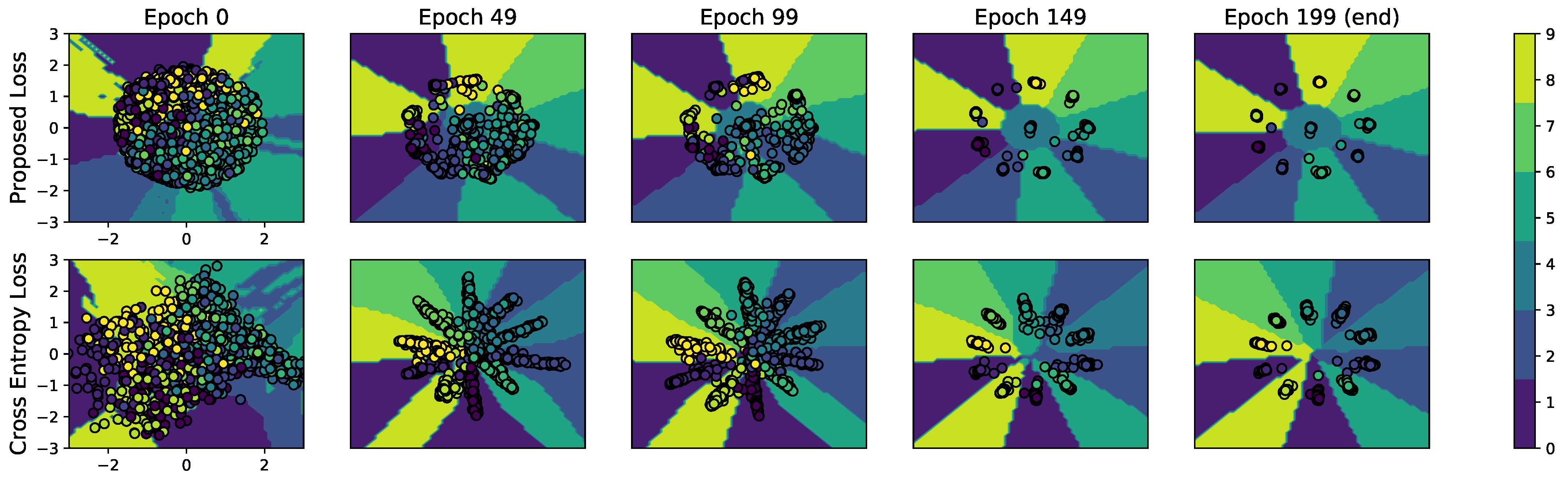
We depict in Figure A1 a comparison between the evolution of the 2D-embeddings obtained by the label variation and the cross-entropy losses when training on the CIFAR-10 dataset. Note that the label variation method allows us to directly train 2D-embeddings, while we had to add a bottleneck layer of the same dimension to the architecture using cross entropy. The figure shows that training examples are better clustered at the end of the training process when using the proposed loss (as compared with using the cross-entropy loss) and that the final embedding is closer to the initial one for the label variation loss. As a matter of fact, label variation is built on top of the initial distribution of data points at the output of the network, whereas cross-entropy forces the output to converge to arbitrarily chosen anchor points (target vector) in that output space. More details on this experiment are available in Reference [14].
Figure A1.
Two-dimensional-Embeddings of the CIFAR-10 training set on a DNN learned using the label variation loss (top row) and the cross-entropy loss (bottom row). Both networks have the same architecture and hyperparameters.
Figure A1.
Two-dimensional-Embeddings of the CIFAR-10 training set on a DNN learned using the label variation loss (top row) and the cross-entropy loss (bottom row). Both networks have the same architecture and hyperparameters.

References
- Tan, M.; Le, Q.V. Efficientnet: Rethinking model scaling for convolutional neural networks. arXiv 2019, arXiv:1905.11946. [Google Scholar]
- Edunov, S.; Ott, M.; Auli, M.; Grangier, D. Understanding back-translation at scale. arXiv 2018, arXiv:1808.09381. [Google Scholar]
- Goodfellow, I.; Bengio, Y.; Courville, A. Deep Learning; MIT Press: Cambridge, MA, USA, 2016. [Google Scholar]
- LeCun, Y.; Bengio, Y.; Hinton, G. Deep learning. Nature 2015, 521, 436–444. [Google Scholar] [CrossRef] [PubMed]
- LeCun, Y. The Power and Limits of Deep Learning. Res.-Technol. Manag. 2018, 61, 22–27. [Google Scholar] [CrossRef]
- Cisse, M.; Bojanowski, P.; Grave, E.; Dauphin, Y.; Usunier, N. Parseval networks: Improving robustness to adversarial examples. In Proceedings of the International Conference on Machine Learning, Sydney, Australia, 6–11 August 2017. [Google Scholar]
- Hendrycks, D.; Dietterich, T. Benchmarking Neural Network Robustness to Common Corruptions and Perturbations. In Proceedings of the International Conference on Learning Representations, New Orleans, LA, USA, 6–9 May 2019. [Google Scholar]
- Lassance, C.; Gripon, V.; Ortega, A. Laplacian Networks: Bounding Indicator Function Smoothness for Neural Networks Robustness. In Proceedings of the APSIPA Transactions on Signal and Information Processing, 8 January 2021. to appear. [Google Scholar]
- Park, W.; Kim, D.; Lu, Y.; Cho, M. Relational Knowledge Distillation. In Proceedings of the IEEE Conference on Computer Vision and Pattern Recognition, Long Beach, CA, USA, 16–20 June 2019; pp. 3967–3976. [Google Scholar]
- Lassance, C.; Bontonou, M.; Hacene, G.B.; Gripon, V.; Tang, J.; Ortega, A. Deep geometric knowledge distillation with graphs. In Proceedings of the ICASSP 2020–2020 IEEE International Conference on Acoustics, Speech and Signal Processing (ICASSP), Barcelona, Spain, 4–8 May 2020; pp. 8484–8488. [Google Scholar]
- Hinton, G.; Vinyals, O.; Dean, J. Distilling the knowledge in a neural network. In Proceedings of the Neural Information Processing Systems 2014 Deep Learning Workshop, Montreal, QC, Canada, 8–13 December 2014. [Google Scholar]
- Koratana, A.; Kang, D.; Bailis, P.; Zaharia, M. LIT: Learned intermediate representation training for model compression. In Proceedings of the International Conference on Machine Learning, Long Beach, CA, USA, 9–15 June 2019; pp. 3509–3518. [Google Scholar]
- Hermans, A.; Beyer, L.; Leibe, B. In defense of the triplet loss for person re-identification. arXiv 2017, arXiv:1703.07737. [Google Scholar]
- Bontonou, M.; Lassance, C.; Hacene, G.B.; Gripon, V.; Tang, J.; Ortega, A. Introducing Graph Smoothness Loss for Training Deep Learning Architectures. In Proceedings of the 2019 IEEE Data Science Workshop (DSW), Minneapolis, MN, USA, 2–5 June 2019; pp. 160–164. [Google Scholar]
- Svoboda, J.; Masci, J.; Monti, F.; Bronstein, M.; Guibas, L. PeerNets: Exploiting Peer Wisdom Against Adversarial Attacks. In Proceedings of the International Conference on Learning Representations, New Orleans, LA, USA, 6–9 May 2019. [Google Scholar]
- Qian, H.; Wegman, M.N. L2-Nonexpansive Neural Networks. In Proceedings of the International Conference on Learning Representations, New Orleans, LA, USA, 6–9 May 2019. [Google Scholar]
- He, K.; Zhang, X.; Ren, S.; Sun, J. Deep residual learning for image recognition. In Proceedings of the IEEE Conference on Computer Vision and Pattern Recognition, Las Vegas, NV, USA, 27–30 June 2016; pp. 770–778. [Google Scholar]
- Krizhevsky, A.; Sutskever, I.; Hinton, G.E. Imagenet classification with deep convolutional neural networks. In Proceedings of the Advances in neural information processing systems, Lake Tahoe, NV, USA, 3–6 December 2012; pp. 1097–1105. [Google Scholar]
- Shuman, D.I.; Narang, S.K.; Frossard, P.; Ortega, A.; Vandergheynst, P. The emerging field of signal processing on graphs: Extending high-dimensional data analysis to networks and other irregular domains. IEEE Signal Process. Mag. 2013, 30, 83–98. [Google Scholar] [CrossRef] [Green Version]
- Kipf, T.N.; Welling, M. Semi-supervised classification with graph convolutional networks. arXiv 2016, arXiv:1609.02907. [Google Scholar]
- Vialatte, J.C. On Convolution of Graph Signals and Deep Learning on Graph Domains. Ph.D. Thesis, IMT Atlantique, Nantes, France, 2018. [Google Scholar]
- Gama, F.; Isufi, E.; Leus, G.; Ribeiro, A. Graphs, Convolutions, and Neural Networks: From Graph Filters to Graph Neural Networks. IEEE Signal Process. Mag. 2020, 37, 128–138. [Google Scholar] [CrossRef]
- Wu, Z.; Pan, S.; Chen, F.; Long, G.; Zhang, C.; Philip, S.Y. A comprehensive survey on graph neural networks. IEEE Trans. Neural Networks Learn. Syst. 2020. [Google Scholar] [CrossRef] [PubMed] [Green Version]
- Liu, Y.; Cao, J.; Li, B.; Yuan, C.; Hu, W.; Li, Y.; Duan, Y. Knowledge Distillation via Instance Relationship Graph. In Proceedings of the IEEE Conference on Computer Vision and Pattern Recognition, Long Beach, CA, USA, 16–20 June 2019; pp. 7096–7104. [Google Scholar]
- Lee, S.; Song, B. Graph-based knowledge distillation by multi-head attention network. arXiv 2019, arXiv:1907.02226. [Google Scholar]
- Anirudh, R.; Bremer, P.; Sridhar, R.; Thiagarajan, J. Influential Sample Selection: A Graph Signal Processing Approach; Technical Report; Lawrence Livermore National Lab. (LLNL): Livermore, CA, USA, 2017. [Google Scholar]
- Gripon, V.; Ortega, A.; Girault, B. An Inside Look at Deep Neural Networks using Graph Signal Processing. In Proceedings of the ITA, San Diego, CA, USA, 11–16 February 2018. [Google Scholar]
- Romero, A.; Ballas, N.; Kahou, S.E.; Chassang, A.; Gatta, C.; Bengio, Y. Fitnets: Hints for thin deep nets. In Proceedings of the International Conference on Learning Representations, San Diego, CA, USA, 7–9 May 2015. [Google Scholar]
- Veličković, P.; Cucurull, G.; Casanova, A.; Romero, A.; Lio, P.; Bengio, Y. Graph attention networks. arXiv 2017, arXiv:1710.10903. [Google Scholar]
- Hu, Y.; Gripon, V.; Pateux, S. Exploiting Unsupervised Inputs for Accurate Few-Shot Classification. arXiv 2020, arXiv:2001.09849. [Google Scholar]
- Ruder, S. An overview of multi-task learning in deep neural networks. arXiv 2017, arXiv:1706.05098. [Google Scholar]
- Dietterich, T.G.; Bakiri, G. Solving multiclass learning problems via error-correcting output codes. J. Artif. Intell. Res. 1994, 2, 263–286. [Google Scholar] [CrossRef] [Green Version]
- Szegedy, C.; Vanhoucke, V.; Ioffe, S.; Shlens, J.; Wojna, Z. Rethinking the inception architecture for computer vision. In Proceedings of the IEEE Conference on Computer Vision and Pattern Recognition, Las Vegas, NV, USA, 27–30 June 2016. [Google Scholar]
- Goodfellow, I.J.; Shlens, J.; Szegedy, C. Explaining and harnessing adversarial examples. arXiv 2014, arXiv:1412.6572. [Google Scholar]
- Madry, A.; Makelov, A.; Schmidt, L.; Tsipras, D.; Vladu, A. Towards Deep Learning Models Resistant to Adversarial Attacks. In Proceedings of the International Conference on Learning Representations, Vancouver, BC, Canada, 30 April–3 May 2018. [Google Scholar]
- Hacene, G.B. Processing and Learning Deep Neural Networks on Chip. Ph.D. Thesis, Ecole Nationale Supérieure Mines-Télécom Atlantique, Nantes, France, 2019. [Google Scholar]
- Frankle, J.; Carbin, M. The Lottery Ticket Hypothesis: Finding Sparse, Trainable Neural Networks. In Proceedings of the International Conference on Learning Representations, New Orleans, LA, USA, 6–9 May 2019. [Google Scholar]
- Belkin, M.; Niyogi, P. Laplacian eigenmaps for dimensionality reduction and data representation. Neural Comput. 2003, 15, 1373–1396. [Google Scholar] [CrossRef] [Green Version]
- Zagoruyko, S.; Komodakis, N. Wide residual networks. arXiv 2016, arXiv:1605.07146. [Google Scholar]
- Krizhevsky, A.; Hinton, G. Learning Multiple Layers of Features from Tiny Images. 2009. Available online: https://www.cs.toronto.edu/~kriz/learning-features-2009-TR.pdf (accessed on 15 January 2021).
- Kalofolias, V.; Perraudin, N. Large Scale Graph Learning From Smooth Signals. In Proceedings of the International Conference on Learning Representations, New Orleans, LA, USA, 6–9 May 2019. [Google Scholar]
- Shekkizhar, S.; Ortega, A. Graph Construction from Data by Non-Negative Kernel Regression. In Proceedings of the ICASSP 2020–2020 IEEE International Conference on Acoustics, Speech and Signal Processing (ICASSP), Barcelona, Spain, 4–8 May 2020; pp. 3892–3896. [Google Scholar]
- Torralba, A.; Fergus, R.; Freeman, W.T. 80 Million Tiny Images: A Large Data Set for Nonparametric Object and Scene Recognition. IEEE Trans. Pattern Anal. Mach. Intell. 2008, 30, 1958–1970. [Google Scholar] [CrossRef] [PubMed]
Figure 1.
Simplified depiction of a residual network (Resnet) with eight residual blocks.

Figure 2.
Graph representation example of 20 examples from CIFAR-10, from the input space (left) to the penultimate layer of the network (right). The different vertex colors represent the classes of the data points. To help the visualization, we only depict the edges that are important for the variation measure (i.e., edges between elements of distinct classes). Note how there are many more edges at the input (a) and how the number of edges decrease as we go deeper in the architecture (b,c).

Table 1.
Error rate comparison on CIFAR-10 for knowledge distillation (KD) methods.
| Method | Error | Gain | Relative Size |
|---|---|---|---|
| Teacher | 7.27% | — | 100% |
| Baseline (student without KD) | 10.34% | — | 27% |
| RKD-D [9] | 10.05% | 0.29% | 27% |
| GKD (Ours) [10] | 9.71% | 0.63% | 27% |
Table 2.
Comparison between the cross-entropy and label variation functions. Best results are presented in bold font.
Table 2.
Comparison between the cross-entropy and label variation functions. Best results are presented in bold font.
| Cost Function | Clean Test Error | Relative MCE |
|---|---|---|
| Cross-entropy | 5.06% | 100 |
| Label Variation (ours) [14] | 5.63% | 90.33 |
Table 3.
Comparison of different methods on their clean error rate and robustness. Best results are presented in bold font.
Table 3.
Comparison of different methods on their clean error rate and robustness. Best results are presented in bold font.
| Metric | Error Rate | Relative MCE | |
|---|---|---|---|
| Method | Clean | Adversarial Attack [34] | Corruptions [7] |
| Baseline | 11.1% | 66.3% | 100 |
| Parseval [6] | 10.3% | 55.0% | 104.4 |
| Label variation regularizer (ours) [8] | 13.2% | 49.5% | 97.6 |
Publisher’s Note: MDPI stays neutral with regard to jurisdictional claims in published maps and institutional affiliations. |
© 2021 by the authors. Licensee MDPI, Basel, Switzerland. This article is an open access article distributed under the terms and conditions of the Creative Commons Attribution (CC BY) license (http://creativecommons.org/licenses/by/4.0/).
Share and Cite
MDPI and ACS Style
Lassance, C.; Gripon, V.; Ortega, A. Representing Deep Neural Networks Latent Space Geometries with Graphs. Algorithms 2021, 14, 39. https://0-doi-org.brum.beds.ac.uk/10.3390/a14020039
AMA Style
Lassance C, Gripon V, Ortega A. Representing Deep Neural Networks Latent Space Geometries with Graphs. Algorithms. 2021; 14(2):39. https://0-doi-org.brum.beds.ac.uk/10.3390/a14020039
Chicago/Turabian StyleLassance, Carlos, Vincent Gripon, and Antonio Ortega. 2021. "Representing Deep Neural Networks Latent Space Geometries with Graphs" Algorithms 14, no. 2: 39. https://0-doi-org.brum.beds.ac.uk/10.3390/a14020039
Note that from the first issue of 2016, this journal uses article numbers instead of page numbers. See further details here.