Article

Simulation-Optimization Approach for Multi-Period Facility Location Problems with Forecasted and Random Demands in a Last-Mile Logistics Application

by
Markus Rabe
1,
Jesus Gonzalez-Feliu
2,
Jorge Chicaiza-Vaca
1,* and
Rafael D. Tordecilla
3,4
1
IT in Production and Logistics, Faculty of Mechanical Engineering, TU Dortmund, 44227 Dortmund, Germany
2
Centre de Recherche en Intelligence et Innovation Managériales, Excelia Business School, 17000 La Rochelle, France
3
IN3—Computer Science Department, Universitat Oberta de Catalunya, 08018 Barcelona, Spain
4
School of Engineering, Universidad de La Sabana, 53753 Chia, Colombia
*
Author to whom correspondence should be addressed.
Submission received: 14 December 2020 / Revised: 18 January 2021 / Accepted: 24 January 2021 / Published: 28 January 2021
(This article belongs to the Special Issue Simulation-Optimization in Logistics, Transportation, and SCM)

Abstract

:
The introduction of automated parcel locker (APL) systems is one possible approach to improve urban logistics (UL) activities. Based on the city of Dortmund as case study, we propose a simulation-optimization approach integrating a system dynamics simulation model (SDSM) with a multi-period capacitated facility location problem (CFLP). We propose this integrated model as a decision support tool for future APL implementations as a last-mile distribution scheme. First, we built a causal-loop and stock-flow diagram to show main components and interdependencies of the APL systems. Then, we formulated a multi-period CFLP model to determine the optimal number of APLs for each period. Finally, we used a Monte Carlo simulation to estimate the costs and reliability level with random demands. We evaluate three e-shopper rate scenarios with the SDSM, and then analyze ten detailed demand configurations based on the results for the middle-size scenario with our CFLP model. After 36 months, the number of APLs increases from 99 to 165 with the growing demand, and stabilizes in all configurations from month 24. A middle-demand configuration, which has total costs of about 750 , 000 €, already locates a suitable number of APLs. If the budget is lower, our approach offers alternatives for decision-makers.

1. Introduction

Last-mile logistics (LML) is known as the least efficient and most complex part of the supply chain. LML activities have negative impacts on pollution and traffic congestion in urban areas [1]. The growth of e-commerce activities has increased the number of individual home deliveries, thus driving up LML flows. Improving the efficiency of LML in urban areas through research is an important driver for the success of e-commerce and helps to reduce the negative externalities associated with urban logistics (UL).
An automated parcel locker (APL) is a potential solution to LML challenges. In our current work, we analyze the use of APLs such as packstations or locker boxes as a promising alternative to improve UL activities [2]. An APL is a group of electronic lockers with variable opening codes. APLs can be used by different consumers whenever it is convenient for them. APLs are located near consumers’ homes, workplaces, and train stations, where online shoppers deliver or ship packages. The costs of home delivery and the related risk of missed delivery are likely to be higher compared APL systems. Online shoppers are likely to use APLs more often in the future [3]. Third-party logistics providers such as DHL, InPost, Norway Post, UPS, or Amazon continue to invest in APLs to gain a competitive advantage [3]. The general overview of experiences with APLs is presented in [1,4]. APLs have several advantages, such as less traffic in city centers, out-of-hours deliveries, fewer kilometers and stops, and cost reductions for e-retailers and delivery companies [5]. Unattended delivery could reduce the number of failed deliveries [4,6,7]. In addition, the use of APLs also offers environmental benefits, such less pollutant emissions [8]. Furthermore, online shoppers are free to choose any pickup time for their parcels, and they can use it as both a delivery and a collection point to return unsatisfactory items. However, APLs have some disadvantages, such as limited payment flexibility in situ, limited storage space, and susceptibility to crime or vandalism [6].
Despite the advantages of the APL concept, from a scientific point of view this strategy has not been discussed sufficiently in the field of LML [9]. Urban parcel deliveries need to be studied in more detail. Most current research shows that the simulation of system dynamics (SD) applied in the LML field [10] is almost completely missing. In the available publications, local visions are adopted without a systemic or holistic perspective. Most of these did not take into account the different viewpoints of stakeholders, processes, interactions, and others [7,11]. Furthermore, for online buyers, the location of APLs is important to decide on their use [6,7]. Many studies have focused on analyzing the savings potential of using APLs, but have not addressed network design issues such as their number and review the associated installation costs. In this paper, we focus on a challenging and appropriate approach to analyze a number of APL configurations in an uncertain demand environment.
Different methods can be used for decision support in UL [1,12], such as empirical approaches, statistical analyses, or integrated computer science models and algorithms, to name a few. As for the last category of methods, researchers use simulation and optimization (SO) techniques as separate approaches in the field of operational research to solve complex problems [13]. On the one hand, exploring the behavior of systems and estimating their response to various environmental changes is a main purpose of using simulation [14]. On the other hand, optimization seeks to solve logistic problems, minimize total costs of ownership, or maximize profit. However, in real complex systems there are very specific properties that make it almost impossible to address the complexity of the problem with only one specific approach. Therefore, it is better to develop models that reflect the complexity of real systems and combine different modeling approaches. This type of combination is called a hybrid modeling approach [15]. By combining different modeling approaches, a hybrid model could provide a more comprehensive and holistic view of the system and a useful approach to understanding complexity. Moreover, according to the authors of [16] a good model is the one that is not only solved with a relevant method (and has an internal coherence and robustness proven), but also the one that represents the reality it aims to relate to in a satisfactory way with respect to the stakeholders that will use it and the decisions it involves. Given that, hybrid methods allow firstly for involving different capabilities, as they result of mixing different methods (so taking the advantages of each involved method). Second, hybrid methods can highlight synergies between the involved methods, as well as complements, aiming at a better representation of a reality [17].
This paper deals with the case of the city of Dortmund, which is located in the federal state North Rhine-Westphalia, Germany. With a population of about 600 , 000 people, it is the seventh largest city in Germany and the 34th largest city in the European Union. Based on the case study, we propose an SO approach as a hybrid model that integrates a system dynamics simulation model (SDSM) with a multi-period capacitated facility location problem (CFLP). We propose this integrated model as a decision support tool for future APL implementations as a last-mile distribution scheme. The paper is structured as follows. First, we use an SDSM to understand the behavior of the components of APL systems with respect to the specific customers and characteristics of the city of Dortmund. A planning horizon of three years (divided into months) is considered. Second, the problem is modeled as a multi-period CFLP. Taking into account the needs to be satisfied by the users, the goal is to find the minimum number of APLs to be installed per month within the time horizon. Several scenarios from the SDSM are considered and solved, taking into account different estimates for the requirements. Third, the performance of the associated solutions in a stochastic environment is evaluated using a Monte Carlo simulation. Finally, the conclusions present possible future work and applications.

2. Related Work

2.1. System Dynamics Modeling

The System Dynamics (SD) methodology was developed by Jay W. Forrester [18]. SD was originally introduced to facilitate the understanding of industrial processes. SD is used as a methodological approach to explain the effects of decisions in complex dynamic systems. The SD approach emphasizes time functions [19,20]. SD Models undergo constant interaction, continuous questioning, testing, and refinement. Based on the feedback concepts of control theory, the SD methodology generates the dynamic behavior of the associated model. The feedback loop structure of systems is represented by causal loop diagrams (CLD) [19,21]. A feedback loop contains two or more causality-related variables that are self-contained. The variable relationships in the loop can be either positive or negative. A positive relationship means that when one variable increases, the other one increases, too. In a balanced relationship, the change in the variables is inverse. The stock and flow diagram (SFD) is the underlying physical structure of the system. The SFD is normally structured according to the CLD. The stock (level) represents the state of the system and the flow (rate) is changed by decisions based on the state of the system. The stock and flow structure (including feedback) of a system determines the quantitative modes of behavior that the system can adopt. For the development of an SD model, the work in [19] presents a modeling process with the following steps: (i) problem analysis, (ii) system conceptualization, (iii) model formulation, (iv) simulation and verification, and (v) policy analysis and improvement. Figure 1 illustrates the SDSM process.
In the context of logistics, some studies show the application of SD to LML activities. In [22], the authors analyzed the decisions and interdependencies between customers, retailers, and suppliers using an SD model from an economic perspective. In [23], the authors applied an SD approach to model interdependencies of decisions by various stakeholders and their impact on city logistics. In [24], the authors presented a specific SD application in UL operations. They also used an SD model in [25] to understand customer behavior from an LML perspective. Although modeling efforts are important in urban logistics [12,26], the simulation seems to be still in the development phase [10]. The most popular simulation approaches remain multi-agent approaches [10,27]. While SD is still preliminary in its applications for urban freight distribution, it has great potential because it can take into account the complexity of the dynamics and heterogeneity of the systems [23].

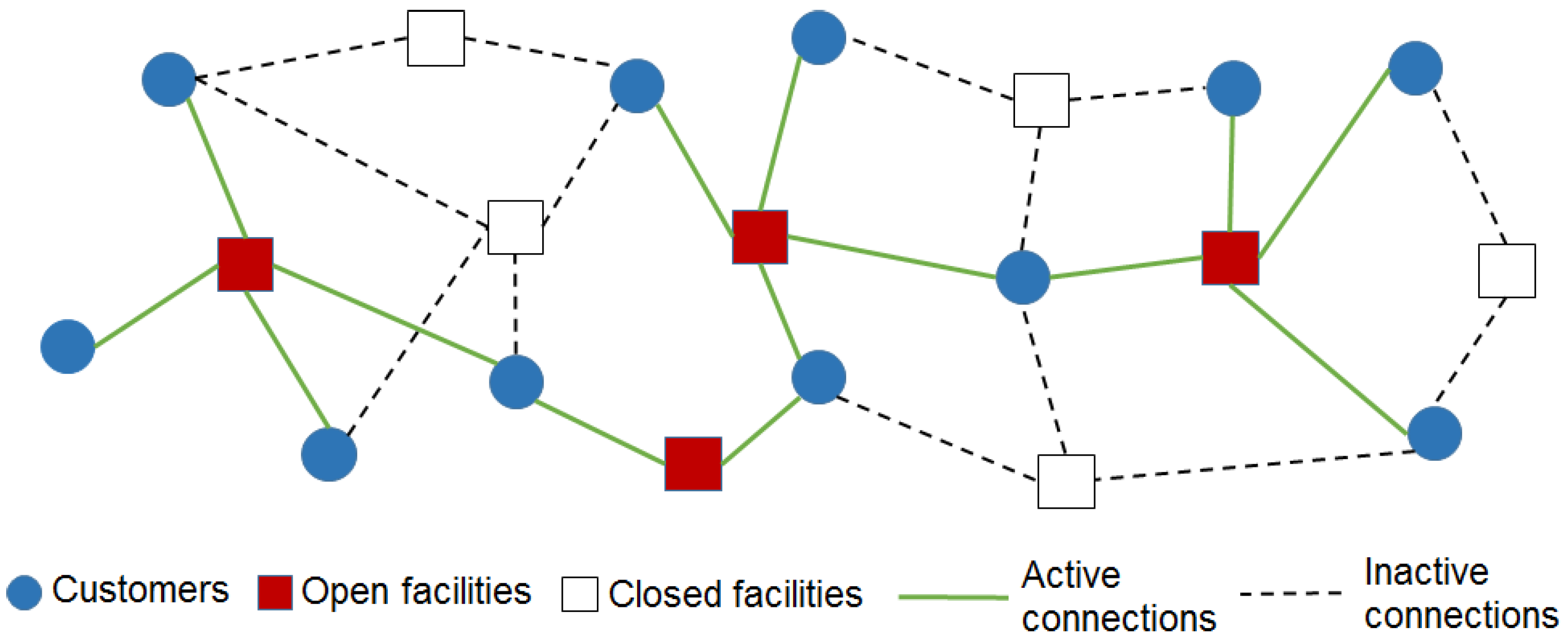
2.2. Facility Location Problems

Facility location determination is a critical strategic business decision. There are several factors that determine facility location, including competition, costs, and associated impacts. The facility location decision has a profound impact on tactical and operational operations. For dealing with this strategic decision, the Facility Location Problem (FLP) was introduced to the field of operations research in the 1960s [28] and was initially called the Plant Location Problem.
FLPs consist of determining the optimal location for one or more facilities to serve a range of demand points. The importance of the optimal location depends on the nature of the problem in terms of the constraints and optimality criteria considered for the site [29]. FLPs are useful for determining the location of facilities such as hospitals, fire stations, bus stops, train stations, truck terminals, gas stations, blood bank centers, retail stores, neighborhoods, libraries, parks, post offices, airports, and landfills. The FLP can be seen as a generalization of the vehicle routing problem with fixed costs for the installation of facilities. An exhaustive review and discussion of the FLPs is provided in [30].
In a basic formulation, the FLP consists of a number of potential plant locations at which a plant can be opened and a number of demand points that must be served. The aim is to determine what subset of facilities needs to be opened in order to minimize the total costs of delivering goods to customers plus the sum of the facility opening costs. A simple example of a classic FLP instance is shown in Figure 2, where each customer (blue circle) is assigned to the nearest open facility (red square) via an active connection.
One of the most frequently investigated discrete location problems is the uncapacitated facility location problem (UFLP). The UFLP is the problem of determining the best location for a given facility—or the best locations for a given group of facilities—given some limitations on the environment in which it can be placed. This contrasts with the capacitated FLP, where facilities limit the number of customers they can serve. In the uncapacitated version, there is no such limitation. Some applications of FLP in UL context are presented in [31,32,33,34,35,36,37,38].

2.3. Monte Carlo Simulation

Monte Carlo simulation (MCS) generates distributions of possible result values. By using probability distributions, variables can have different probabilities of different outcomes occurring. Probability distributions are a suitable way to describe the uncertainty in variables of a risk analysis. During an MCS process, values are randomly selected from input probability distributions. Each set of samples is called an iteration, and the result of that sample is recorded. MCS conducts this hundreds or thousands of times, and the result is a probability distribution of possible outcomes. In this way, MCS provides a much more complete prediction of what may happen because it also delivers the probability that it will happen [39].
Many quantitative problems in science, engineering, and finance are solved today with MCS techniques. We list some important application areas, such as industrial engineering and operations research, physical processes, economics and finance, computer-based statistics and parallel computing, adaptive Monte Carlo Algorithms, spatial processes, and quasi Monte Carlo [40]. The MCS has been applied to last mile logistics in the real-world, which depends on many external random factors. This is especially true for last-mile deliveries. Challenging factors include—but are not limited to—traffic, weather, and the size of individual orders. To this end, MCS has found great use in assessing the risk and reliability of supply chains.

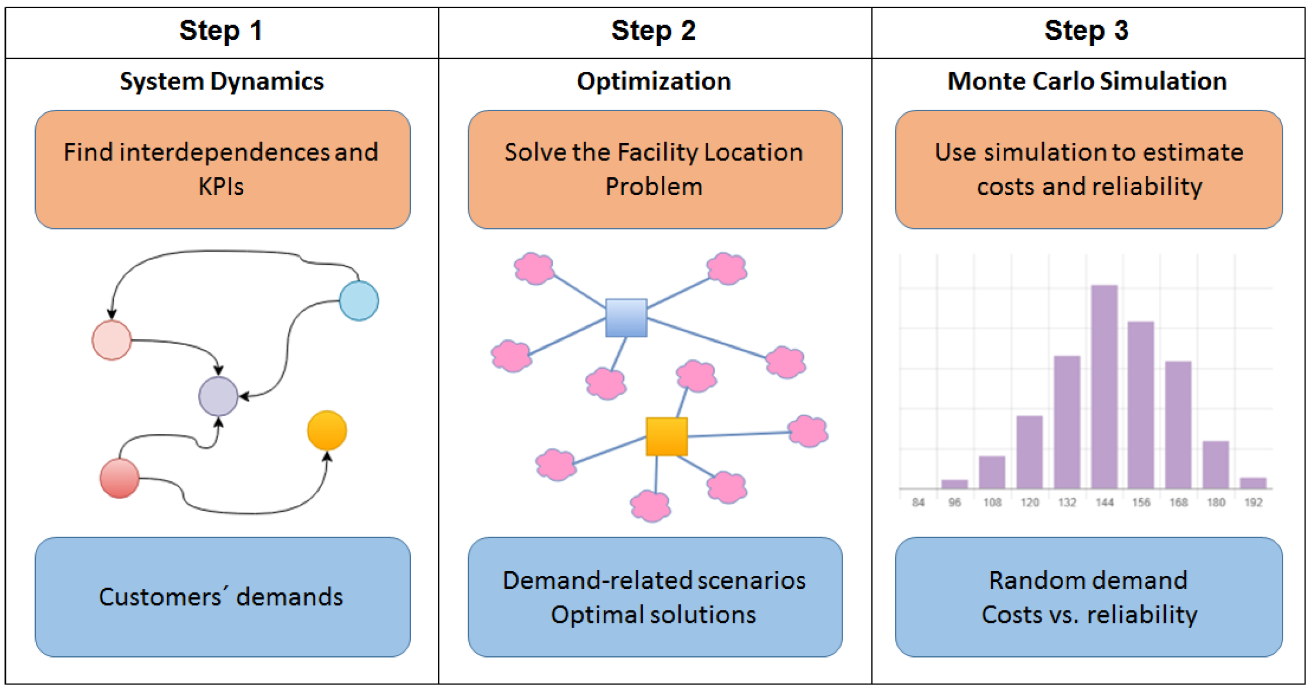
3. Integrated Simulation-Optimization Approach

Hybrid models play an important role in most real-world systems. Multiple perspectives can be obtained, each of which can answer a different important question. For answering the range of questions that can be asked with respect to a system, a combined set of model types can be the answer. Hybrid methods can bring more comprehensive and efficient estimations of a reality by enhancing the synergies among different methods and giving the suitable output for decision-makers [41]. One of the main goals of the SO method as a hybrid model is to efficiently address both the optimization and the uncertainty. An overview of the application of SO methods in designing resilient supply chain networks is presented in [42]. There are many ways to combine simulation and optimization, and the appropriate design depends strongly on the properties of the problem. The guideline 3633.12 [43] by the German Association of Engineers (Verein Deutscher Ingenieure (VDI)) provides a classification for different combinations of simulation and optimization in terms of sequential and hierarchical combination, which has been in detail elaborated by the Arbeitsgemeinschaft Simulation (ASIM) in Germany [44]. A sequential combination assumes that either simulation or optimization is completed before the other one can be executed. Within a hierarchical combined approach that can be called several times during the overall execution. Moreover, the details of the main classifications of various SO combinations are described in [13]. According to their classifications, we consider an analytical model improvement approach, where simulation is used to improve the model results, either by refining its parameters or by extending them, e.g., by considering different scenarios. In this context, the SDSM, based on an SO concept for APLs presented in [45], provides a suitable methodology to determine the behavior of the parameters in our multi-period capacitated FLP model. A well-proven SO approach to solve this kind of problems is provided by simheuristic algorithms [46,47].
In particular, our approach consists of the following steps, which are shown in Figure 3: (i) for each district, we use the SDSM to generate an estimate of expected demand; (ii) for different scenarios, each scenario being defined by a different level of demand (e.g., lower than expected, as expected, or higher than expected), solve the associated CFLP model; and (iii) use a Monte Carlo simulation to evaluate the solutions obtained in the previous step when used in a stochastic environment. Here, we assumed that the demand per district is uncertain and follows a known probability distribution, with the aim of comparing total costs with the reliability.

4. Application in the City of Dortmund

This paper deals with the case of the city of Dortmund, which is divided into 62 districts, codified from 000 to 960. Figure 4 shows the map of the city of Dortmund with its respective districts.

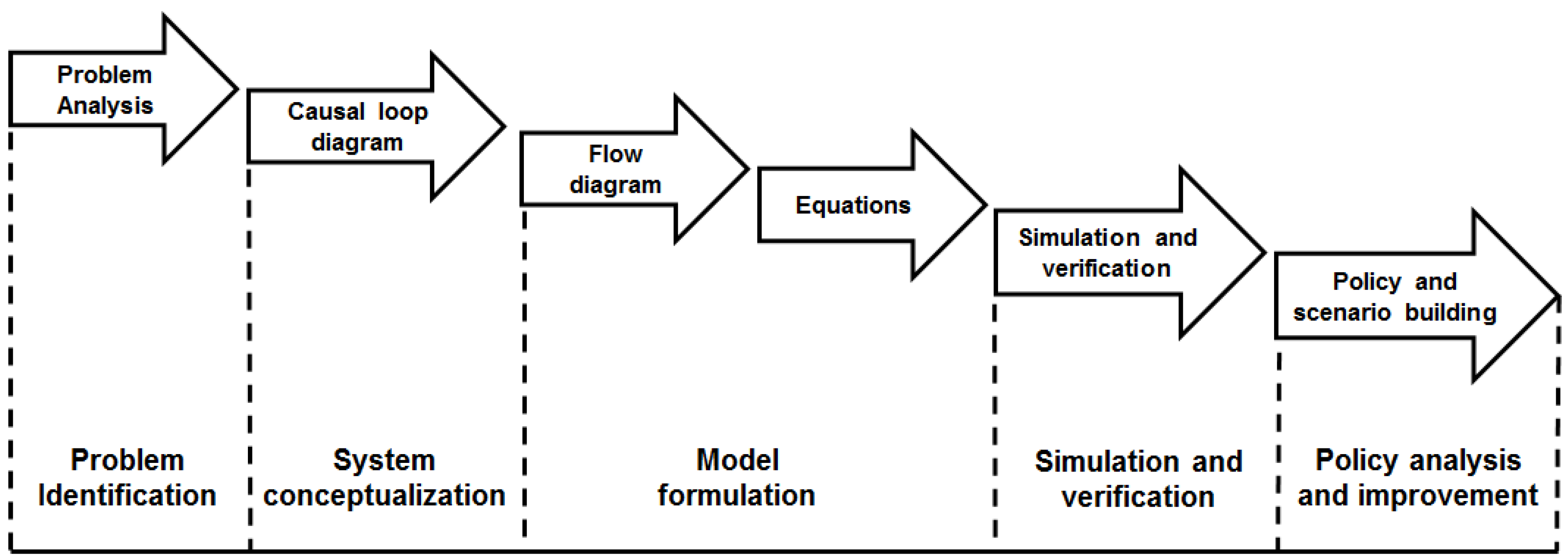
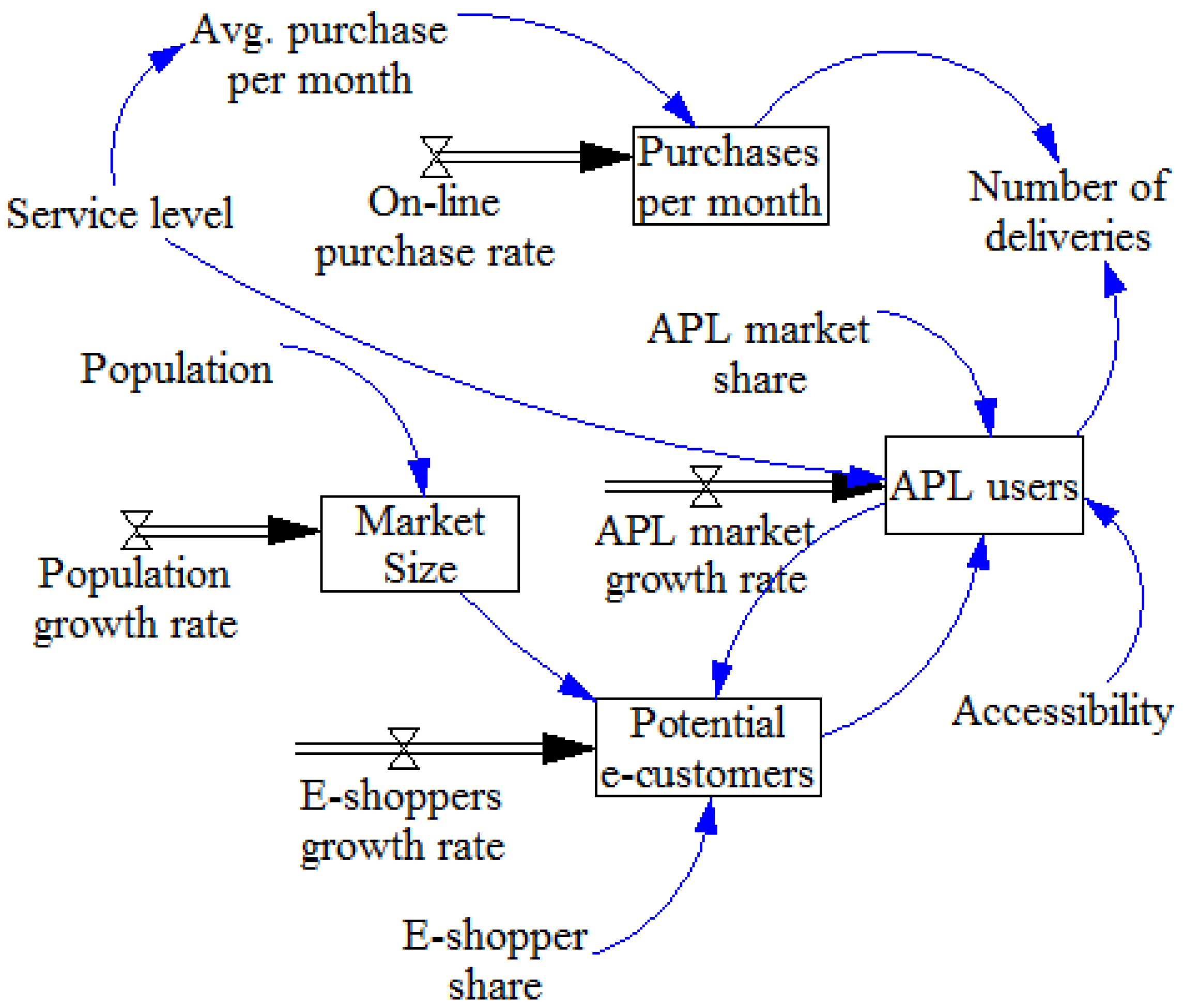
4.1. System Dynamics Simulation Model

We propose an SDSM for APL as a UL delivery scheme. The SDSM is designed to understand the behavior of components of APL systems, and it will be used as a decision support for future implementations. To develop an SD model, we followed the steps shown in Figure 1.

4.1.1. Problem Identification

E-commerce does not necessarily mean the absence of physical shops, but rather an evolution in the way retailers carry out orders. For this reason, e-commerce has led to an increase in innovative combinations of physical and digital solutions, resulting in different ways of preparing, distributing, and collecting orders from customers [48]. Examples include home delivery, collection points, and APLs. We focus on understanding APL systems as a UL delivery scheme in the context of e-commerce and evaluating its components over time.

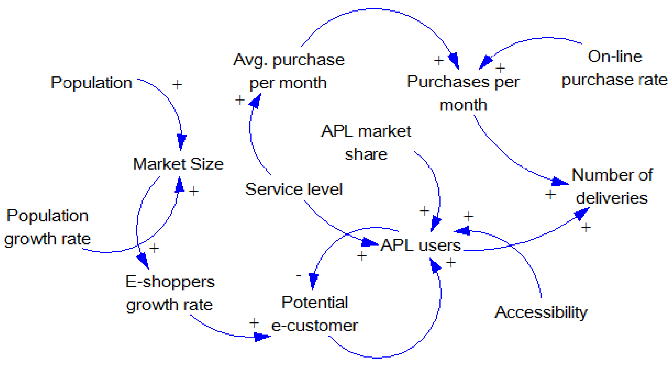
4.1.2. System Conceptualization

From a qualitative point of view, we use an SDSM to understand the behavior and interdependencies of the components of APL systems. From the existing literature on APLs (mainly based on case studies and field data), we define the main components that have an impact on the system. Following SD standard procedures [19], we use the software tool Vensim to create the causal-loop and stock-flow diagrams. Figure 5 describes the main APL system components that third-party logistics service providers will need to consider for future APL applications.
The CLD describes that the market size is positively influenced by the population and the population growth rate. The potential number of e-customers is positively influenced by the e-shoppers growth rate and balanced by the number of APL users. In turn, the number of deliveries is positively reinforced by purchases per month and number of APL users. In turn, the purchases per month are positively reinforced by the average purchases per month and the online purchase rate.

4.1.3. Model Formulation

From a quantitative perspective, we present the evaluation of the APL components. Based on the CLD, we built the SFD, as shown in Figure 6. First, the variables of market size, potential e-customers, purchases per month, and APL users are defined as stocks (squared). Then, population growth rate, e-shoppers growth rate, online purchase rate, and APL market growth rate are defined as flows. Finally, population, accessibility, service level, average purchase per month, APL market share, and number of deliveries are auxiliary variables. The main output in this model is the number of deliveries, which are used as input values in the FLP model.

4.1.4. Simulation and Verification

We apply the SDSM based on public data of the city of Dortmund and using the e-commerce trends in the German context. Taking into account the volatility of the e-commerce sector, the SDSM evaluates the system components of APL for a planning horizon of three years (divided into 36 months). Table 1 shows the components used in the SDSM application and their values.

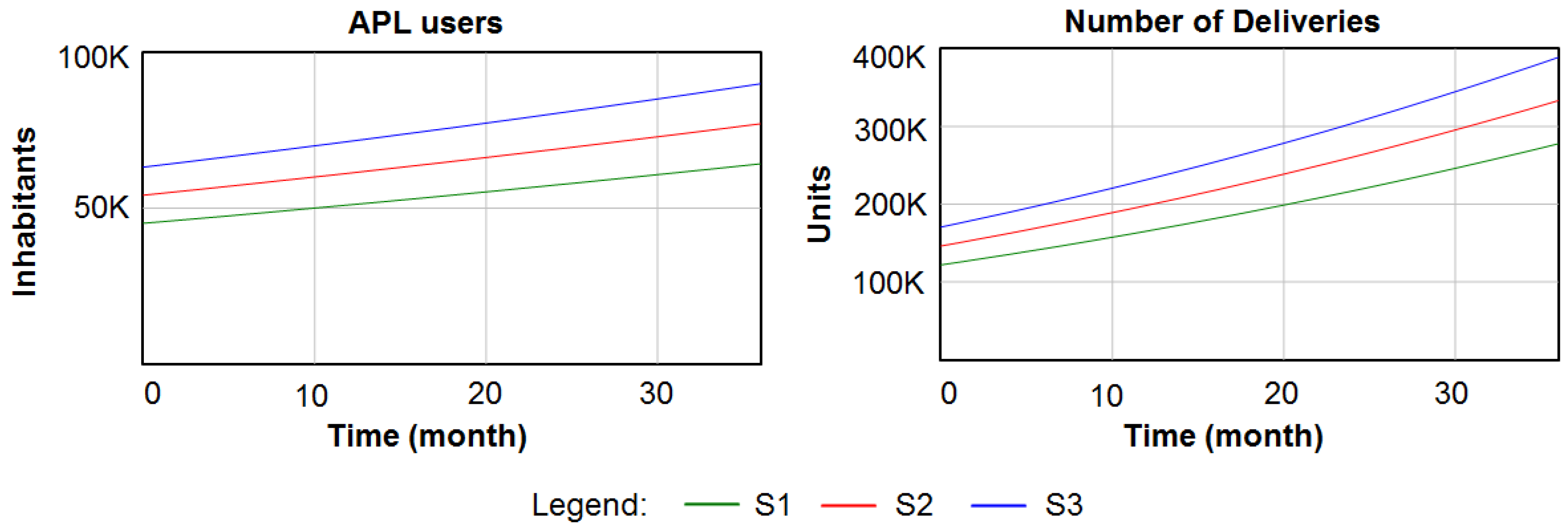
4.1.5. Policy Analysis and Scenario Building

Table 2 shows the significant changes in the e-shoppers rate to build the scenarios. We consider Scenario 1 (S1), Scenario 2 (S2), and Scenario 3 (S3) with increasing rates of e-shoppers.

4.2. Multi-Period Facility Location Problem

The FLP is a well-known optimization challenge where the typical goal is to find the minimum costs and location of facilities that must be open to meet customer requirements, either deterministically [30] or stochastically [31,49]. If routing decisions are also included, the FLP turns into the so-called location routing problem [50,51]. In general, FLPs are classified either as capacitated or uncapacitated. The former refers to the case where the facilities have a known limit to the demand they can meet. The latter is the case where the service capacity of each facility exceeds the total demand of customers. Figure 7 illustrates the capacitated FLP (CFLP) for the APL network in the city of Dortmund. Here, each district is a potential APL location (yellow square) and each APL is connected to each other in the APLs configuration (dashed lines). These connections are used to calculate the distance matrix between districts.
A multi-period CFLP is taken into account in our work. Decisions made in a given period affect future periods over a time horizon of T. In particular, as demand is expected to increase in future periods, we assume that whenever an APL is opened within a period t T , it must remain open until the end of the time horizon, i.e., for all t T : t > t . Similarly, third-party logistics providers indicate that a minimum percentage of m ( 0 , 1 ) of total installed capacity must be used. Therefore, with the set I of nodes representing all districts in the city, each district i I could contain no, one, or more APLs, each with a known capacity a i > 0 . Similarly, each district j I has an aggregated demand in the period t T , d j t > 0 . For two districts i , j I , the unit costs of assigning an APL located in the district i to a customer located in the district j is c i j > 0 . Similarly, the costs of opening an APL in district i I during the period t T is indicated as f i t > 0 . In this context, the binary variable x i j t takes the value 1 if customers in the district j I are assigned to an APL in the district i I during the period t T ; otherwise, the value is 0. Similarly, the integer variable y i t represents the number of APLs that are open in district i I and in period t T . Then, our multi-period CFLP can be formulated as follows.
M i n i m i z e i I j I t T c i j d j t x i j t + i I t T f i t ( y i t y i t 1 )
subject to:
i I x i j t = 1 j I , t T
y i t y i t 1 i I , t T \ { 1 }
j I d j t x i j t a i y i t i I , t T
j I d j t m i I a i y i t t T
x i j t { 0 , 1 } i I , j I , t T
y i t Z + i I , t T
The expression (1) indicates the objective function that minimizes the total costs: The first term indicates the service costs of APLs, while the second represents the fixed costs of opening new APLs in the time horizon. Constraints (2) ensure that for each period t T and each district j I exactly one APL is assigned. Restrictions (3) ensure that once an APL is opened, it remains open until the end of the time horizon. Constraints (4) ensure that for each APL in district i I and time period t T , the demand served by that APL does not exceed its capacity. Constraints (5) guarantee a minimum utilization percentage of the total installed capacity of APLs for each t T period. Finally, constraints (6) and (7) specify the ranges of the decision variables.

5. Computational Results and Discussion

Based on the city of Dortmund as a real-world case, a set of experiments considering a 36-month planning horizon has been tested. Table 1 shows the parameters provided by the SDSM. It yields multiple outputs, from which the yearly demand per district is the most relevant one to feed the multi-period CFLP model. Then, the integrated SO approach described in Section 3 is applied to obtain a set of solutions assessed in terms of stochastic cost and reliability level.

5.1. System Dynamics Simulation Model Results

The market size increases in line with the population growth rate from from 602,666 in month 1 to 606,182 inhabitants in month 36. The purchases per month, the number of deliveries and the number of APLs show an increasing trend over time. The number of deliveries increases from 125 , 353 to 277 , 910 packages per month. We applied the SDSM and changed the average purchases per month as shown in Table 2. The results for APL users in the first month are 45,666 for S 1 , 54,799 for S 2 , and 63,933 for S 3 , and at the 36th month 64,331 for S 1 , 77,202 for S 2 , and 90,071 for S 3 . The results of the number of deliveries (units) in the first month are 125,353 for S 1 , 150,423 for S 2 , and 175,496 for S 3 , and in the 36th month 277,910 for S 1 , 333,512 for S 2 , and 389,106 for S 3 . Figure 8 illustrates the scenario comparison of the users of APL and the number of deliveries. The complete results generated by the SDSM of the default scenarios are shown in Table A1, Table A2 and Table A3 in Appendix A.

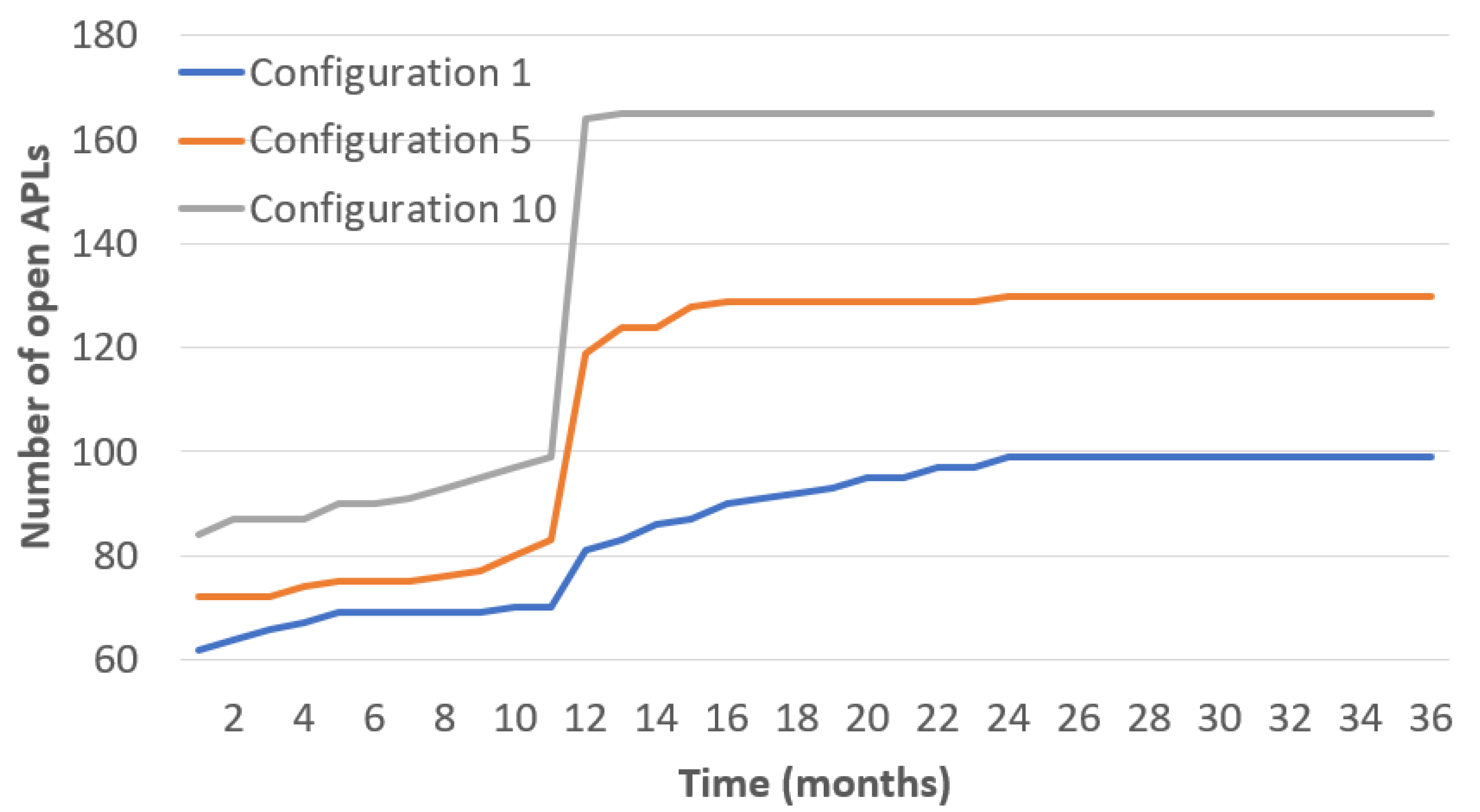
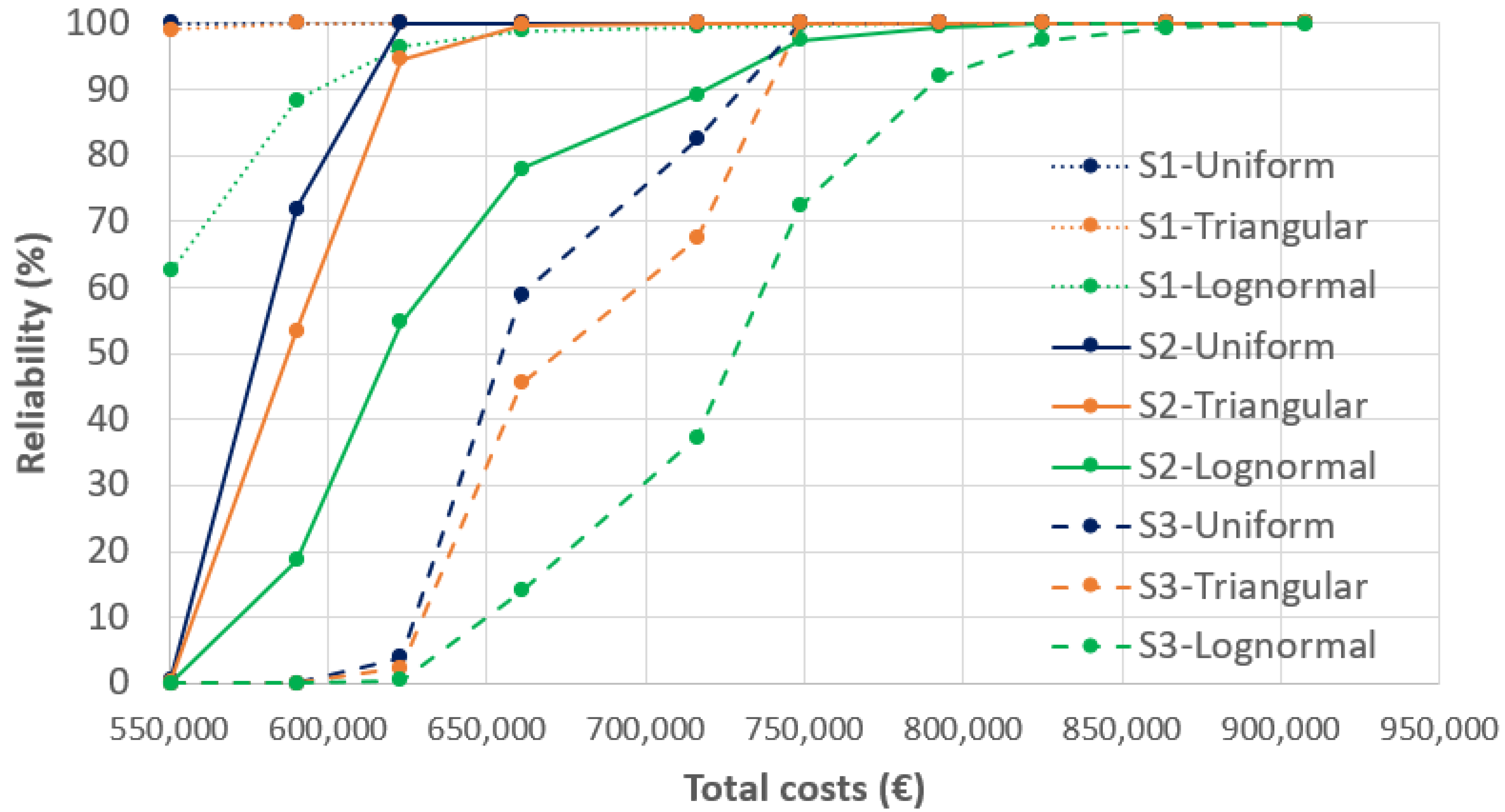
5.2. Generating and Simulating Optimal Configurations

As soon as our SDSM provides the number of deliveries (expected demand) for the three scenarios ( s S , where S = { S 1 , S 2 , S 3 } ) under consideration of Table 2, are used to feed our CFLP model. We evaluate ten APL network configurations ( k K , where K = { 1 , 2 , , 10 } ) with the demand increasing proportional to k, based on the scenario S2. Each configuration is obtained by optimally solving the CFLP model using the procedure described below.
  • Consider a uniformly distributed random demand D j t k per district j J during the period t T for generating the configurations.
  • Define μ j t = E [ D j t k ] and assume that μ j t is the medium demand corresponding to the scenario S 2 .
  • Define a factor δ = 0.01 to increase the size of the uniform interval as we move forward into future periods.
  • Generate the random demand using Equation (8). The expression 1 + k 1 | K | 1 is useful to increase μ j t proportionally to the value of k. In this way, we guarantee that generated configurations differ in size.
    D j t k U 1 + k 1 | K | 1 ( 1 δ t ) μ j t , 1 + k 1 | K | 1 ( 1 + δ t ) μ j t j I , t T , k K
The variable costs c i j are proportional to the distance between each pair of districts. They were estimated using a web mapping service. The fixed costs are f i t = 5500 € for the first year and each district, and increase according to an average inflation rate of 2 % per year. The capacity of each APL in a district i I is a i = 6000 units per month, and the minimum utilization percentage is m = 40 % . Then, our CFLP model is solved with Cplex for all ten configurations. The number of resulting open APLs per month is shown in Figure 9 for three out of these configurations. The lowest and highest lines represent solutions for the lowest and highest demand, respectively. The rest of the solutions are in between. As the demand μ j t increases over time, the number of open APLs will behave the same regardless of the configuration. However, this consistent behavior does not extend beyond the year 1 for k = 10 and beyond the year 2 for k = 1 and k = 5 , when the total installed APLs are sufficient to cover the total demand by the end of the planning horizon. Furthermore, there is a sharp increase in open APLs from months 11 to 12. This behavior is caused by two parameters: The annual growth of the fixed costs f i t drives the APLs that are opened when they are less expensive, but always limited by the minimum utilization percentage m. Finally, the total number of APLs installed varies significantly from one scenario to another, for example, while 165 APLs are required for k = 10 , only 99 APLs are installed in the configuration k = 1 at the end of the planning horizon. All configuration results are stored in Table A4, Table A5 and Table A6 in Appendix B.
Once all configurations have been generated, they are tested in a stochastic environment, assuming that the demand per district is uncertain and follows a known probability distribution. Consider a random demand D j t s whose mean and standard deviation are μ j t s and σ j t s , respectively, per district j J during the period t T for the scenario s S . We assume that μ j t s is the demand generated by our SDSM. Now, as the goal is to evaluate the performance of each configuration, they must be tested under the same demand conditions; therefore, the demand does not depend further on the configuration. Then, D j t s is simulated and each configuration is evaluated in terms of total costs (Equation (1)) and reliability. Studies on reliability in supply chains are found in [52,53]. We define the reliability R k s of the configuration k K for the scenario s S as the probability that the stochastic demand of all districts in the city can be successfully satisfied, i.e.,
R k s = 1 b k s n · 100 % k K , s S
where b k s is the total number of simulation runs where the configuration does not cover all district demands, and n is the total number of runs. In other words, if at least one APL in a configuration is not able to cover all assigned needs, that configuration will fail. In our experiments, a total of n = 5000 runs are performed for each combination of scenario s and configuration k. Without losing generality, we assume that demand is independent of the customers’ district, but our methodology can easily be adapted to take into account correlated demand. For the realization of the demand, three probability distributions have been tested:
  • A uniform distribution, according to Equation (10). In this case, σ j t s = 3 3 δ t μ j t s .
    D j t s U 1 δ t μ j t s , 1 + δ t μ j t s
  • A symmetric triangular distribution, according to Equation (11), i.e., the mode equals μ j t s . To obtain conditions similar to 1, the lower and upper limits of this distribution are calculated assuming that the standard deviation is equal.
    D j t s T 1 2 δ t μ j t s , μ j t s , 1 + 2 δ t μ j t s
  • A lognormal distribution, according to Equation (12). Again, the standard deviation is the same as in the point 1 to preserve similar conditions.
    D j t s L o g n o r m a l μ j t s , σ j t s
Figure 10 shows the main results of the simulation process for each configuration. Blue, orange, and green lines represent the results from the demand for uniform, triangular, or log-normal distribution. In addition, dotted, solid, and dashed lines represent the results for the scenarios S 1 (low demand), S 2 (medium demand), and S 3 (high demand), respectively. Each dot on each line represents a single configuration. In general, more expensive configurations result in higher reliability, because they include a larger number of installed APLs. When the demand follows either a uniform or a triangular distribution, the most expensive half of the configurations always achieve a 100.0 % reliability level, regardless of the scenario. In other words, the configuration k = 6 , with total costs of 748,660€, already locates a suitable number of APLs and eliminates the need to consider more expensive configurations. However, if the budget is lower, our approach offers other good alternatives for the decision makers.
In general, configurations are less reliable when demand scenarios are increased. For example, configuration k = 4 , with total costs of 661,100€, only achieves a reliability level of 14.0 % under the high demand scenario and a log-normal distribution. Conversely, this configuration achieves a reliability level of 98.8 % under the low demand scenario. Furthermore, the reliability is very sensitive to the probability distribution. Broadly speaking, a configuration fails if the demand is too high (Equation (9)). Therefore, configurations simulating a log-normal demand, which has no upper limit, are less reliable than those where the probability distribution is either uniform or triangular (Equations (10) and (11)). This fact underlines the relevance of integrating the study to determine the behavior of demand in the real case.

6. Conclusions

With the goal of determining the optimal number and location of automated parcel locker (APL) systems in a multi-period time horizon, this paper has proposed the use of an integrated simulation-optimization approach combining system dynamics with exact optimization and Monte Carlo simulation. We propose this integrated model as a decision support tool for future APL implementations as a last-mile distribution scheme. The analysis is based on a real-world case study where service requirements are considered as random variables that evolve over time. First, a system dynamics simulation model is designed to determine the 36-month performance of parameters such as APL users and number of deliveries. Then, these results feed a multi-period facility location model that provides the optimal number of APLs. To deal with the demand uncertainty, different scenarios are considered and solved with precise methods. The solutions associated with each scenario are then sent to a Monte Carlo simulation to estimate both their costs and reliability level.
The model provides an optimal number of APLs, taking into account the expectations of user demands. We have considered three scenarios S 1 , S 2 , and S 3 for 50%, 60%, and 70% of the e-shopper rate. The results for the number of deliveries (units) after 36 months show a wide range of shipments from about 277,000 in S 1 to nearly 400,000 in S 3 . We used our CFLP to evaluate ten APL network configurations ( k = 1 , , 10 ) with increasing demand in relation to each scenario. Obviously, there is a strong impact on the number of APLs that the city needs. After 36 months, the number of APLs increases from 99 in the case of the lowest demand to 165 at maximum demand. Interestingly, the number of APLs stabilizes from month 24 in all configurations. Thus, we can conclude that the effect on APLs appears linear in relation to the potential users of APL with no obvious scale effects. From a stochastic environment, we assumed that the demand per district is uncertain and follows a known probability distribution. Whenever the demand follows either a uniform or a triangular distribution, the most expensive configurations always reach a reliability level of 100.0 % regardless of the scenario. The configuration k = 6 , with total costs of 748,660€, already locates a suitable number of APLs. However, if the budget is lower, our approach offers other alternatives for decision makers.
All in all, the work illustrates the potential of combining different simulation and optimization techniques to correctly address complex optimization problems in real urban logistics, where uncertainties must also be taken into account. The following research lines are still open for the future: (i) increasing the level of detail on the demand side, taking into account correlated and individual customers’ demands instead of aggregated ones—which will significantly increase the size of the problem; (ii) develop a metaheuristic-based approach for the optimization phase, as this will be a necessary step when larger instances are to be analyzed; and (iii) extend the approach to a fully simheuristic algorithm, so that the feedback provided by the Monte Carlo simulation can be reused to guide the metaheuristic search.

Author Contributions

Conceptualization, M.R., J.G.-F., and J.C.-V.; methodology, J.C.-V. and R.D.T.; software, J.C.-V. and R.D.T.; validation, J.C.-V. and R.D.T.; formal analysis, M.R. and J.G.-F.; writing—original draft preparation, J.C.-V. and R.D.T.; writing—review and editing, M.R. and J.G.-F. All authors have read and agreed to the published version of the manuscript.

Funding

This work has been partially supported by the German Academic Exchange Service (DAAD) Research Grants—Doctoral Programmes in Germany, 2017/18.

Institutional Review Board Statement

Not applicable.

Informed Consent Statement

Not applicable.

Data Availability Statement

Data are available upon reasonable request to the corresponding author.

Conflicts of Interest

The authors declare no conflict of interest.

Appendix A. Results Generated by the SDSM for the Horizon Planning in the Proposal Scenarios

Appendix A shows the results by the SDSM for the first three years.
Table A1. Results generated by the SDSM in the first year.
Output
Parameter
Month
123456789101112
Market size (thousands)
S 1 602.6 602.7 602.8 602.9 603 603.1 603.2 603.3 603.4 603.5 603.6 603.7
S 2 602.6 602.7 602.8 602.9 603 603.1 603.2 603.3 603.4 603.5 603.6 603.7
S 3 602.6 602.7 602.8 602.9 603 603.1 603.2 603.3 603.4 603.5 603.6 603.7
Potential e-customers (thousands)
S 1 303.4 305.5 307.6 309.7 311.9 314 316.1 318.5 320 322.4 324.5 326.6
S 2 364.1 366.6 369.2 371.7 374.3 376.8 379.3 381.9 384.4 386.9 389.4 391.9
S 3 424.7 427.7 430.7 433.7 436.6 439.6 442.6 445.5 448.5 451.4 454.3 457.3
APL users (thousands)
S 1 45.6 46.1 46.6 47.1 47.5 48 48.5 49 49.5 50 50.5 51.1
S 2 54.7 55.3 55.9 56.6 57.1 57.7 58.2 58.8 59.4 60.1 60.7 61.3
S 3 63.9 64.6 65.2 65.9 66.6 67.3 68 68.7 69.4 70.1 70.8 71.5
Number of deliveries (thousands)
S 1 125.3 128.7 132.1 135.6 139.2 142.8 146.4 150.1 153.9 157.7 161.6 165.5
S 2 150.4 154.4 158.6 162.8 167 171.3 175.7 180.2 184.7 189.3 193.9 198.6
S 3 175.4 180.2 185 189.9 194.9 199.9 205 210.2 215.5 220.8 226.3 231.8
Table A2. Results generated by the SDSM in the second year.
Output
Parameter
Month
131415161718192021222324
Market size (thousands)
S 1 603.8 603.9 604 604.1 604.2 604.3 604.4 604.5 604.6 604.7 604.8 604.9
S 2 603.8 603.9 604 604.1 604.2 604.3 604.4 604.5 604.6 604.7 604.8 604.9
S 3 603.8 603.9 604 604.1 604.2 604.3 604.4 604.5 604.6 604.7 604.8 604.9
Potential e-customers (thousands)
S 1 328.7 330.8 332.9 334.9 337 339.1 341.2 343.2 345.3 347.3 349.425 351.4
S 2 394.4 396.9 399.4 401.9 404.4 406.9 409.4 411.9 414.3 416.8 419.3 421.7
S 3 457.3 460.2 463.1 466 468.9 471.8 474.7 477.6 480.5 483.4 486.3 489.1
APL users (thousands)
S 1 51.6 52.1 52.6 53.1 53.7 54.2 54.7 55.3 55.8 56.3 56.9 57.4
S 2 61.9 62.5 63.1 63.8 64.4 65 65.7 66.3 67 67.6 68.3 68.9
S 3 72.2 72.9 73.7 74.4 75.1 75.9 76.6 77.4 78.1 78.9 79.7 80.4
Number of deliveries (thousands)
S 1 169.5 173.5 177.7 181.8 186 190.3 194.6 199 203.5 208 212.6 217.2
S 2 203.4 208.3 213.2 218.2 223.3 228.4 233.6 238.9 244.2 249.6 255.1 260.7
S 3 237.3 243 248.7 254.6 260.5 266.5 272.5 278.7 284.9 291.3 297.7 304.2
Table A3. Results generated by the SDSM in the third year.
Output
Parameter
Month
252627282930313233343536
Market size (thousands)
S 1 605 605.1 605.2 605.3 605.4 605.5 605.6 605.7 605.8 605.9 606 606.1
S 2 605 605.1 605.2 605.3 605.4 605.5 605.6 605.7 605.8 605.9 606 606.1
S 3 605 605.1 605.2 605.3 605.4 605.5 605.6 605.7 605.8 605.9 606 606.1
Potential e-customers (thousands)
S 1 353.5 355.5 357.5 359.6 361.6 363.6 365.6 367.6 369.6 371.6 373.6 375.6
S 2 424.2 426.6 429 431.5 433.9 436.3 438.8 441.2 443.6 446 448.4 450.8
S 3 494.9 497.7 500 503.4 506.2 509.1 511.9 514.7 517.5 520.3 523.1 525.9
APL users (thousands)
S 1 58 58.5 59.1 59.7 60.2 60.8 61.4 61.9 62.5 63.1 63.7 64.3
S 2 69.6 70.3 70.9 71.6 72.3 73 73.7 74.4 75 75.7 76.4 77.2
S3 81.2 82 82.8 83.6 84.4 85.1 85.9 86.8 87.6 88.4 89.2 90
Number of deliveries (thousands)
S 1 221.9 226.7 231.5 236.4 241.4 246.4 251.5 256.6 261.8 267.1 272.5 277.9
S 2 266.4 272.1 277.9 283.7 289.7 295.7 301.8 308 314.2 320.6 327 333.5
S 3 310.8 317.4 324.2 331338345 352.1 359.3 366.6 374 381.5 389.1

Appendix B. Number of APLs by Period and Configuration

Appendix B shows the results for the required number of APLs for the first three years.
Table A4. Number of APLs in the first year.
Output
Parameter
Month
123456789101112
Number of APLs
k 1 626466676969696969707081
k 2 696969696969707171717392
k 2 6969707070717273737374101
k 4 7171727272737475767676110
k 5 7272727475757576778083119
k 6 7375757676767880828486130
k 7 7576767777818383858790139
k 8 7676788083858889899091148
k 9 8081838687898989909292153
k 10 8487878790909193959799164
Table A5. Number of APLs in the second year.
Output
Parameter
Month
131415161718192021222324
Number of APLs
k 1 838687909192939595979799
k 2 9497100100100102104105105106106107
k 3 102106108110112112113113113113113113
k 4 113113118119119119120120120120120120
k 5 124124128129129129129129129129129130
k 6 132135135135135135135135135135136136
k 7 143144144144144144144144144144144144
k 8 149149149149149149149149149149149150
k 9 157157157157157157157157157157157157
k 10 165165165165165165165165165165165165
Table A6. Number of APLs in the third year.
Output
Parameter
Month
252627282930313233343536
Number of APLs
k 1 999999999999999999999999
k 2 107107107107107107107107107107107107
k 3 113113113113113113113113113113113113
k 4 120120120120120120120120120120120120
k 5 130130130130130130130130130130130130
k 6 135135135135135135135135135135136136
k 7 144144144144144144144144144144144144
k 8 150150150150150150150150150150150150
k 9 157157157157157157157157157157157157
k 10 165165165165165165165165165165165165

References

  1. Gonzalez-Feliu, J. Sustainable Urban Logistics: Planning and Evaluation; ISTE Ltd./John Wiley and Sons Inc.: Hoboken, NJ, USA, 2017. [Google Scholar]
  2. Boudoin, D.; Morel, C.; Gardat, M. Supply Chains and Urban Logistics Platforms. In Sustainable Urban Logistics: Concepts, Methods and Information Systems; Gonzalez-Feliu, J., Semet, F., Routhier, J., Eds.; Springer: New York, NY, USA, 2013; pp. 1–20. [Google Scholar]
  3. Moroz, M.; Polkowski, Z. The Last Mile Issue and Urban Logistics: Choosing Parcel Machines in the Context of the Ecological Attitudes of the Y Generation Consumers Purchasing Online. Transp. Res. Procedia 2016, 16, 378–393. [Google Scholar] [CrossRef] [Green Version]
  4. Zurel, Ö.; van Hoyweghen, L.; Braes, S.; Seghers, A. Parcel Lockers, an Answer to the Pressure on the Last Mile Delivery? In New Business and Regulatory Strategies in the Postal Sector; Parcu, P., Brennan, T., Glass, V., Eds.; Springer International Publishing: Cham, Switzerland, 2018; pp. 299–312. [Google Scholar]
  5. Verlinde, S.; Rojas, C.; Buldeo Rai, H.; Kin, B.; Macharis, C. E-Consumers and Their Perception of Automated Parcel Stations. In City Logistics 3: Towards Sustainable and Liveable Cities; Taniguchi, E., Thompson, R., Eds.; ISTE Ltd./John Wiley and Sons Inc.: Hoboken, NJ, USA, 2018; pp. 147–160. [Google Scholar]
  6. Vakulenko, Y.; Hellstrom, D.; Hjort, K. What’s in the Parcel Locker? Exploring Customer Value in E-commerce Last Mile Delivery. J. Bus. Res. 2018, 88, 421–427. [Google Scholar] [CrossRef]
  7. Iwan, S.; Kijewska, K.; Lemke, J. Analysis of Parcel Lockers’ Efficiency as the Last Mile Delivery Solution—The Results of the Research in Poland. Transp. Res. Procedia 2016, 12, 644–655. [Google Scholar] [CrossRef] [Green Version]
  8. Faulin, J.; Grasman, S.; Juan, A.; Hirsch, P. Sustainable Transportation and Smart Logistics: Decision-Making Models and Solutions; Elsevier: Oxford, UK, 2018. [Google Scholar]
  9. Guerrero, J.; Dıaz-Ramırez, J. A Review on Transportation Last-mile Network Design and Urban Freight Vehicles. In Proceedings of the 2017 International Conference on Industrial Engineering and Operations Management, Bristol, UK, 24–25 July 2017; pp. 533–552. [Google Scholar]
  10. Jlassi, S.; Tamayo, S.; Gaudron, A. Simulation Applied to Urban Logistics: A State of the Art. In City Logistics 3: Towards Sustainable and Liveable Cities; Taniguchi, E., Thompson, R., Eds.; ISTE Ltd./John Wiley and Sons Inc.: Hoboken, NJ, USA, 2018; pp. 32–58. [Google Scholar]
  11. Morganti, E.; Dablanc, L.; Fortin, F. Final Deliveries for Online Shopping: The Deployment of Pickup Point Networks in Urban and Suburban Areas. Res. Transp. Bus. Manag. 2014, 11, 23–31. [Google Scholar] [CrossRef] [Green Version]
  12. Gonzalez-Feliu, J. (Ed.) Logistics and Transport Modeling in Urban Goods Movement; IGI Global: Hershey, PA, USA, 2019. [Google Scholar]
  13. Figueira, G.; Almada-Lobo, B. Hybrid Simulation-Optimization Methods: A Taxonomy and Discussion. Simul. Model. Pract. Theory 2014, 46, 118–134. [Google Scholar] [CrossRef] [Green Version]
  14. Crainic, T.G.; Perboli, G.; Rosano, M. Simulation of Intermodal Freight Transportation Systems: A Taxonomy. Eur. J. Oper. Res. 2018, 270, 401–418. [Google Scholar] [CrossRef]
  15. Martinez-Moyano, I.; Macal, C. A Primer for Hydrid Modeling and Simulation. In Proceedings of the 2016 Winter Simulation Conference (WSC), Washington, DC, USA, 11–14 December 2016; Roeder, T.M., Frazier, P.I., Szechtman, R., Zhou, E., Huschka, T., Chick, S.E., Eds.; Institute of Electrical and Electronics Engineers, Inc.: Piscataway, NJ, USA, 2016; pp. 133–147. [Google Scholar]
  16. Ackoff, R.L. Optimization + Objectivity = Optout. Eur. J. Oper. Res. 1977, 1, 1–7. [Google Scholar] [CrossRef]
  17. Le Bouthillier, A.; Crainic, T.G. A Cooperative Parallel Metaheuristic for the Vehicle Routing Problem with Time Windows. Comput. Oper. Res. 2005, 32, 1685–1708. [Google Scholar] [CrossRef]
  18. Forrester, J.W. Industrial Dynamics after the First Decade. Manag. Sci. 1968, 14, 398–415. [Google Scholar] [CrossRef] [Green Version]
  19. Sterman, J. Business Dynamics; Irwin/McGraw-Hill: Boston, MA, USA, 2000. [Google Scholar]
  20. Taniguchi, E.; Thompson, R.; Yamada, T. Emerging Techniques for Enhancing the Practical Application of City Logistics Models. Procedia Soc. Behav. Sci. 2012, 39, 3–18. [Google Scholar] [CrossRef] [Green Version]
  21. Bala, B.K.; Arshad, F.M.; Noh, K.M. System Dynamics: Modelling and Simulation; Springer: Singapore, 2017. [Google Scholar]
  22. Villa, S.; Gonçalves, P.; Arango, S. Exploring Retailers’ Ordering Decisions Under Delays. Syst. Dyn. Rev. 2012, 31, 1–27. [Google Scholar] [CrossRef]
  23. Kunze, O.; Wulfhorst, G.; Minner, S. Applying Systems Thinking to City Logistics: A Qualitative (and Quantitative) Approach to Model Interdependencies of Decisions by Various Stakeholders and their Impact on City Logistics. Transp. Res. Procedia 2016, 12, 692–706. [Google Scholar] [CrossRef] [Green Version]
  24. Villa, S.; Gonçalves, P.; Arango, S. Describing and Explaining Urban Freight Transport by System Dynamics. Transp. Res. Procedia 2017, 25, 1075–1094. [Google Scholar]
  25. De La Torre, G.; Gruchmann, T.; Kamath, V.; Melkonyan, A.; Krumme, K. A System Dynamics-Based Simulation Model to Analyze Consumers’ Behavior Based on Participatory Systems Mapping—A “Last Mile” Perspective. In Innovative Logistics Services and Sustainable Lifestyles; Melkonyan, A., Krumme, K., Eds.; Springer Science and Business Media: New York, NY, USA, 2013; pp. 165–194. [Google Scholar]
  26. Anand, N.; van Duin, J.R.; Quak, H.; Tavasszy, L. Relevance of City Logistics Modeling Efforts: A Review. Transp. Rev. 2015, 35, 701–719. [Google Scholar] [CrossRef]
  27. Anand, N.; van Duin, J.R.; Tavasszy, L. Framework for Modeling Multi-Stakeholder City Logistics Domain Using the Agent Based Modeling Approach. Transp. Res. Procedia 2016, 16, 4–15. [Google Scholar] [CrossRef] [Green Version]
  28. Balinski, M.L. Integer Programming: Methods, Uses, Computations. Manag. Sci. 1965, 12, 253–313. [Google Scholar] [CrossRef]
  29. Laporte, G.; Nickel, S.; Saldanha da Gama, F. Location Science; Springer International Publishing: Cham, Switzerland, 2015. [Google Scholar]
  30. Melo, M.T.; Nickel, S.; Saldanha-da-Gama, F. Facility Location and Supply Chain Management—A Review. Eur. J. Oper. Res. 2009, 196, 401–412. [Google Scholar] [CrossRef]
  31. De Armas, J.; Juan, A.; Marquès, J.M.; Pedroso, J.P. Solving the Deterministic and Stochastic Uncapacitated Facility Location Problem: From a Heuristic to a Simheuristic. J. Oper. Res. Soc. 2017, 68, 1161–1176. [Google Scholar] [CrossRef]
  32. Absi, N.; Feillet, D.; Garaix, T.; Guyon, O. The City Logistics Facility Location Problem. In Proceedings of the ODYSSEUS 2012, Fifth International Workshop on Freight Transportation and Logistics, Mykonos Island, GR, USA, 21–25 May 2012. [Google Scholar]
  33. Pamučar, D.; Vasin, L.; Atanasković, P.; Miličić, M. Planning the City Logistics Terminal Location by Applying the Green-Median Model and Type-2 Neurofuzzy Network. Comput. Intell. Neurosci. 2016, 2016. [Google Scholar] [CrossRef] [Green Version]
  34. Sopha, B.M.; Asih, A.M.S.; Pradana, F.D.; Gunawan, H.E.; Karuniawati, Y. Urban Distribution Center Location: Combination of Spatial Analysis and Multi-Objective Mixed-Integer Linear Programming. Int. J. Eng. Bus. Manag. 2016, 8. [Google Scholar] [CrossRef] [Green Version]
  35. Dell’Amico, M.; Novellani, S. A Two-Echelon Facility Location Problem with Stochastic Demands for Urban Construction Logistics: An Application within the SUCCESS Project. In Proceedings of the 2017 IEEE International Conference on Service Operations and Logistics, and Informatics (SOLI), Bari, Italy, 18–20 September 2017; pp. 90–95. [Google Scholar]
  36. Gan, M.; Li, D.; Wang, M.; Zhang, G.; Yang, S.; Liu, J. Optimal Urban Logistics Facility Location with Consideration of Truck-Related Greenhouse Gas Emissions: A Case Study of Shenzhen City. Math. Probl. Eng. 2018, 2018. [Google Scholar] [CrossRef]
  37. Nataraj, S.; Ferone, D.; Quintero-Araujo, C.; Juan, A.; Festa, P. Consolidation Centers in City logistics: A Cooperative Approach Based on the Location Routing Problem. Int. J. Ind. Eng. Comput. 2018, 10, 393–404. [Google Scholar] [CrossRef]
  38. Herrmann, E.; Kunze, O. Facility Location Problems in City Crowd Logistics. Transp. Res. Procedia 2019, 41, 117–134. [Google Scholar] [CrossRef]
  39. Brandimarte, P. Handbook in Monte Carlo Simulation: Applications in Financial Engineering, Risk Management, and Economics; John Wiley and Sons.: Hoboken, NJ, USA, 2014. [Google Scholar]
  40. Kroese, D.P.; Brereton, T.; Taimre, T.; Botev, Z.I. Why the Monte Carlo Method is so Important Today. Wiley Interdiscip. Rev. Comput. Stat. 2014, 6, 386–392. [Google Scholar] [CrossRef]
  41. Palacios-Argüello, L.; Gonzalez-Feliu, J.; Gondran, N.; Badeig, F. Assessing the Economic and Environmental Impacts of Urban Food Systems for Public School Canteens: Case Study of Great Lyon Region. Eur. Transp. Res. Rev. 2018, 10, 37. [Google Scholar] [CrossRef] [Green Version]
  42. Tordecilla, R.D.; Juan, A.A.; Montoya-Torres, J.R.; Quintero-Araujo, C.L.; Panadero, J. Simulation-Optimization Methods for Designing and Assessing Resilient Supply Chain Networks under Uncertainty Scenarios: A Review. Simul. Model. Pract. Theory 2021, 106, 102166. [Google Scholar] [CrossRef]
  43. VDI 3633 Part 12. Simulation of Systems in Materials Handling, Logistics, and Production—Simulation and Optimisation; Beuth: Berlin, Germany, 2020. [Google Scholar]
  44. Maerz, L.; Krug, W.; Rose, O.; Weigert, G. (Eds.) Simulation und Optimierung in Produktion und Logistik; Springer: Berlin/Heidelberg, Germany, 2010. [Google Scholar]
  45. Rabe, M.; Chicaiza-Vaca, J. A Simulation-Optimization Conceptual Model of Automated Parcel Lockers on Macro and Micro Planning Levels. In Proceedings of the 2019 Winter Simulation Conference (WSC), National Harbor, MD, USA, 8–11 December 2019; Mustafee, N., Bae, K.-H., Lazarova-Molnar, S., Rabe, M.C., Szabo, C., Haas, P., Son, Y.-J., Eds.; Institute of Electrical and Electronics Engineers, Inc.: Piscataway, NJ, USA, 2019; pp. 2904–2905. [Google Scholar]
  46. Juan, A.; Faulin, J.; Grasman, S.; Rabe, M.; Figueira, G. A Review of Simheuristics: Extending Metaheuristics to Deal with Stochastic Combinatorial Optimization Problems. Oper. Res. Perspect. 2015, 2, 62–72. [Google Scholar] [CrossRef] [Green Version]
  47. Juan, A.A.; Kelton, W.D.; Currie, C.S.; Faulin, J. Simheuristics Applications: Dealing with Uncertainty in Logistics, Transportation, and other Supply Chain Areas. In Proceedings of the 2019 Winter Simulation Conference (WSC), National Harbor, MD, USA, 8–11 December 2019; Rabe, M., Juan, A.A., Mustafee, N., Skoogh, A., Jain, S., Johansson, B., Eds.; Institute of Electrical and Electronics Engineers, Inc.: Piscataway, NJ, USA, 2019; pp. 3048–3059. [Google Scholar]
  48. Durand, B.; Gonzalez-Feliu, J. Urban Logistics and E-grocery: Have Proximity Delivery Services a Positive Impact on Shopping Trips? Procedia Soc. Behav. Sci. 2012, 39, 510–520. [Google Scholar] [CrossRef]
  49. Pages-Bernaus, A.; Ramalhinho, H.; Juan, A.A.; Calvet, L. Designing E-commerce Supply Chains: A Stochastic Facility-location Approach. Int. Trans. Oper. Res. 2019, 26, 507–528. [Google Scholar] [CrossRef]
  50. Quintero-Araujo, C.L.; Caballero-Villalobos, J.P.; Juan, A.A.; Montoya-Torres, J.R. A Biased-randomized Metaheuristic for the Capacitated Location Routing Problem. Int. Trans. Oper. Res. 2017, 24, 1079–1098. [Google Scholar] [CrossRef]
  51. Quintero-Araujo, C.L.; Gruler, A.; Juan, A.A.; Faulin, J. Using Horizontal Cooperation Concepts in Integrated Routing and Facility-location Decision. Int. Trans. Oper. Res. 2019, 26, 551–579. [Google Scholar] [CrossRef]
  52. Adenso-Diaz, B.; Mena, C.; Garcia-Carbajal, S.; Liechty, M. The Impact of Supply Network Characteristics on Reliability. Supply Chain. Manag. Int. J. 2012, 17, 263–276. [Google Scholar] [CrossRef]
  53. Peng, P.; Snyder, L.V.; Lim, A.; Liu, Z. Reliable Logistics Networks Design with Facility Disruptions. Transp. Res. Part B Methodol. 2011, 45, 1190–1211. [Google Scholar] [CrossRef]
Figure 1. Steps to build an system dynamics simulation model (SDSM) based on the work in [19].
Algorithms 14 00041 g001
Figure 2. Illustrative example of the classical FLP based on the work in [31].
Algorithms 14 00041 g002
Figure 3. Schema of the integrated simulation-optimization approach.
Algorithms 14 00041 g003
Figure 4. The map of city of Dortmund with its codified districts.
Algorithms 14 00041 g004
Figure 5. The automated parcel locker (APL) system causal-loop diagram.
Algorithms 14 00041 g005
Figure 6. The APL systems stock-flow diagram.
Algorithms 14 00041 g006
Figure 7. Illustrative CFLP for APLs in the city of Dortmund.
Algorithms 14 00041 g007
Figure 8. Scenario comparison: APL users (left) and number of deliveries (right).
Algorithms 14 00041 g008
Figure 9. Number of total open APLs along the planning horizon for three configurations (k = 1, 5, 10).
Algorithms 14 00041 g009
Figure 10. Optimal solutions evaluated in terms of costs and reliability.
Algorithms 14 00041 g010
Table 1. List and characteristics of variables used on the SDSM of the APL systems
ParameterDefinitionInitial Values
PopulationNumber of inhabitants in city of Dortmund602,566 inhabitants
Population growth rateFactor0.02/12 (%) per month
Market SizePopulation×Population growth ratePopulation
Service levelFactor90 (%)
AccessibilityFactor70 (%)
Potential e-customers(Market Size×E-shopper share-APL users)×Market Size×
E-shoppers growth rateE-shopper share
E-shoppers growth rateFactor0.2/12 (%)
E-shoppers shareFactor50 (%)
APL market shareFactor15 (%)
Avg. purchase per monthConstant×Service level3 units per month
On-line purchase rateFactor10 (%)
Purchases per monthAvg. purchase per e-customer×Avg. purchase
On-line purchase rateper month
APL users(Potential e-customers×APL market share×Potential e-customers
APL market growth rate)××APL market share
(Service level×Accessibility)
Number of deliveriesAPL users×Purchases per month0 Units
Table 2. Value changes to develop the scenarios.
VariableS1S2S3
E-shoppers rate50%60%70%
Publisher’s Note: MDPI stays neutral with regard to jurisdictional claims in published maps and institutional affiliations.

