
Integrated Simulation-Based Optimization of Operational Decisions at Container Terminals


Institute of Maritime Logistics, Hamburg University of Technology, 21073 Hamburg, Germany
*
Author to whom correspondence should be addressed.
†
These authors contributed equally to this work.
Algorithms 2021, 14(2), 42; https://0-doi-org.brum.beds.ac.uk/10.3390/a14020042
Submission received: 6 December 2020
/
Revised: 25 January 2021
/
Accepted: 25 January 2021
/
Published: 28 January 2021
(This article belongs to the Special Issue Simulation-Optimization in Logistics, Transportation, and SCM)
Abstract
:At container terminals, many cargo handling processes are interconnected and occur in parallel. Within short time windows, many operational decisions need to be made and should consider both time efficiency and equipment utilization. During operation, many sources of disturbance and, thus, uncertainty exist. For these reasons, perfectly coordinated processes can potentially unravel. This study analyzes simulation-based optimization, an approach that considers uncertainty by means of simulation while optimizing a given objective. The developed procedure simultaneously scales the amount of utilized equipment and adjusts the selection and tuning of operational policies. Thus, the benefits of a simulation study and an integrated optimization framework are combined in a new way. Four meta-heuristics—Tree-structured Parzen Estimator, Bayesian Optimization, Simulated Annealing, and Random Search—guide the simulation-based optimization process. Thus, this study aims to determine a favorable configuration of equipment quantity and operational policies for container terminals using a small number of experiments and, simultaneously, to empirically compare the chosen meta-heuristics including the reproducibility of the optimization runs. The results show that simulation-based optimization is suitable for identifying the amount of required equipment and well-performing policies. Among the presented scenarios, no clear ranking between meta-heuristics regarding the solution quality exists. The approximated optima suggest that pooling yard trucks and a yard block assignment that is close to the quay crane are preferable.
1. Introduction
Seaports are the interface between various transport modes in the maritime supply chain. In 2019, the volume of global maritime containerized trade had tripled to 152 million TEU (Twenty-foot Equivalent Unit, the size of a standard container) from its value in 1997 [1]. Moreover, ship sizes have also tripled in the past 20 years, from an 8000 TEU capacity to around 24,000 TEU. This implies that, in addition to adjustments to the port’s infrastructure and superstructure, container terminals have to substantially increase their efficiency in ship handling in order to keep unproductive berthing times as short as possible while container volumes that are handled during one ship call increase. Thus, the challenge for terminals is to handle a large number of containers within a very short period of time. Terminals can address this challenge by creating technical prerequisites (i.e., using more and higher-performance equipment) and by optimizing operational processes. While the use of more equipment entails correspondingly more investment and higher running costs, intelligent control of operational processes leads to more efficient cargo handling without additional costs. Therefore, it is reasonable to minimize the amount of necessary equipment and to coordinate operational processes.
Container handling requires a large number of process steps in the terminal. When a ship is berthed, Quay Cranes (QCs) unload the containers and set them onto waiting Yard Trucks (YTs), which then transport them to the storage area. There, Rubber-Tired Gantry (RTGs) cranes lift the containers into the respective Yard Block (YB) for short-term storage until the container is picked up. The steps in the process of loading a ship run in the opposite direction. The processes are coupled because YTs are passive equipment and are not able to lift the containers themselves. As a result, waiting times and utilization of the respective equipment must be weighed against each other. In order to perform ship handling as quickly as possible and to reduce the waiting times of the QCs, it is preferable to use more YTs however, this leads to longer waiting times and lower utilization of YTs. Furthermore, using too many YTs leads to congestion and, therefore, to delays in ship handling [2]. The better the balance between these conflicting objectives, the more efficiently the terminal works.
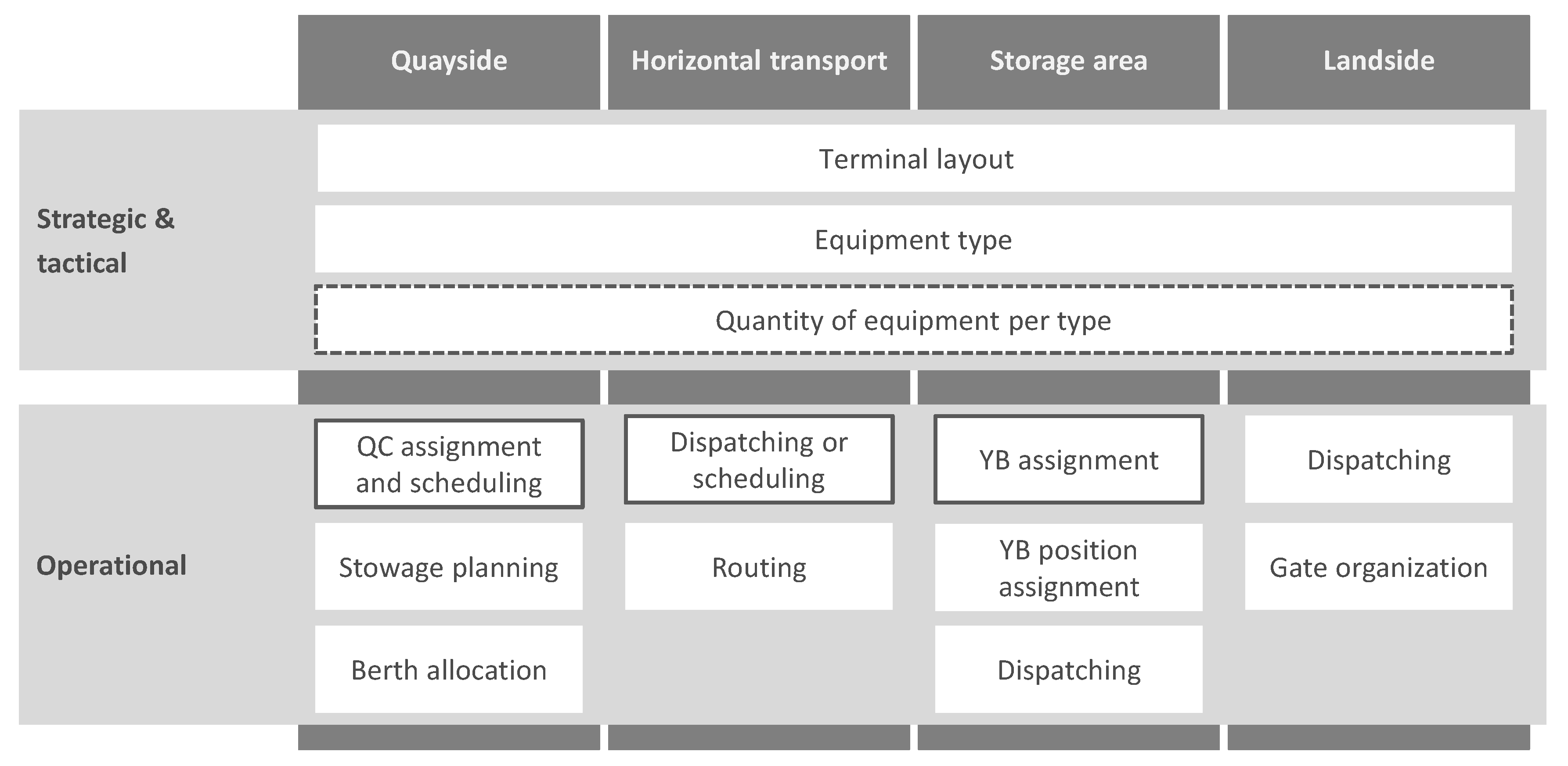
There are several decision problems in the design and operation of container terminals, which strongly influence the efficiency of container handling. Figure 1 shows an overview of typical decision problems at container terminals.
Decisions regarding the design of the terminal layout (e.g., location and size of the YBs) or the equipment that must be used and how much of it to procure have a rather long-term influence (refer to [3] for a recent overview). From a short-term perspective, on the quayside, decisions include berth allocation, stowage planning, and QC assignment and scheduling (refer to [4] for an overview). In horizontal transport, the decision problems are dispatching or scheduling (assigning vehicles and transport orders) and routing. Dispatching (assigning RTGs and storage orders), YB assignment, and YB position assignment are the primary decision problems in the storage area. On the land side, there are also questions of order assignment and gate control. Kizilay and Eliiyi [5] provide a recent overview of container terminal decision problems.
These decision problems influence each other [6]. For example, berth allocation directly influences the YB assignment and vice versa. The distances between the ship at the berth and the assigned YBs should be as short as possible, and at the same time, sufficient YBs should be assigned to a berth or QC. RTGs in the yard can typically move 15 containers within one hour, while QCs have a productivity of around 30 moves/h. Thus, at least two YBs (each being served by at least one RTG) have to be connected to one QC. Another example is the relationship between gate organization and dispatching in the yard: If the number of truck arrivals is regulated by a truck appointment system, then this also influences the number of handling orders for RTGs and thus affects dispatching [7]. These are just two examples of the numerous interactions between decision problems. Therefore, there is a risk that the overall solution will deteriorate if only one decision problem is optimized. Hence, it is necessary to combine the different related decision problems into a single integrated decision problem. Usually, the operations on the waterside are focused on due to the high costs related to the berth time of a ship. This means that the number of QCs, YTs, and RTGs as well as the integration of the handling processes need to be jointly considered to ensure efficient operations. Thus, this study analyzes a combination of QC assignment and dispatching, as well as YB assignment as shown with a dark frame around the respective boxes in Figure 1. Additionally, the dashed frame around the quantity of equipment per type indicates that the number of YTs used is modified.
Integrated decision problems covering QCs, YTs, and RTGs have been traditionally solved by formulating and solving a mathematical model. At first glance, this seems like a reasonable approach. However, this results in a very complex problem for which a solution is difficult to find and, especially under the real-time requirements of a container terminal, is almost impossible to solve in terms of computing power. Therefore, it is worthwhile stepping back and considering different methods, including the use of policies.
1.1. Literature Review on Integrated Decision Problems
There are two main approaches to addressing the operational decision problems of container terminals [8]. The first approach takes into account the complex dynamic environment of a container terminal. It typically uses priority rules, which are analyzed with the help of simulation models that can represent stochastic processes. Simulation models involving container terminals are reviewed in [9,10]. In the second approach, a simplified deterministic mathematical model is formulated. Either the model can be solved optimally for small instances, or an approximation can be found with the help of heuristics.
While the first approach is better suited to volatile processes at container terminals, simulation studies that aim to investigate several decision problems quickly become very complex [11]. The second approach also quickly reaches its limits. In this context, Zhen et al. [12] showed that the integrated QC and YT scheduling problem is non-deterministic polynomial-time hard, which means that the computing time required to optimally solve the problem is too long to be used in practice. To take advantage of both approaches, especially in order to investigate integrated decision problems that influence each other, the approach of combining simulation and optimization has been developed in recent years. He et al. [13] addressed integrated QC, YT, and RTG scheduling. They developed a mixed-integer programming model and proposed a simulation-based optimization method. Their optimization algorithm integrates genetic and particle swarm optimization algorithms. Cao et al. [14] aimed to schedule RTGs and YTs simultaneously in order to decrease the ship turnaround time. They introduced a multi-layer genetic algorithm to solve the scheduling problem and designed an algorithm-accelerating strategy. Castilla-Rodríguez et al. [15] focused on the QC scheduling problem: They integrated artificial intelligence techniques and simulation, combining an evolutionary algorithm with a simulation model to embed uncertainty. Kizilay et al. [16] studied the integrated problem of QC assignment and scheduling, YB assignment, and YT dispatching. They proposed a mixed-integer programming and constraint programming model and showed that the constraint programming model performed much better in terms of calculating time. Integrated quayside problems can also be investigated with other aims, such as saving costs and energy simultaneously [17] or exploring different modes of integration [18]. Sislioglu et al. [19] combined discrete event simulation, data envelopment analysis, and cost-efficiency analysis to investigate different investment alternatives based on the number of QCs, total length of a quay, YTs, and RTGs. They applied their model to 16 different scenarios but did not modify the operating policies. Furthermore, other research has combined different simulation paradigms to solve optimization problems at different decision levels. For example, in [20], a system-dynamic model was used to optimize the main parameters of a dry port, and in [21], a combination of system-dynamic and discrete-event simulation models was used. Kastner et al. [22] provide a literature overview of simulation-based optimization at container terminals. They focused on the covered problems, chosen meta-heuristics, and the shapes of the parameter configuration space in the respective publications. Similarly, Zhou et al. [23] present a summary of publications on the integration of simulation and optimization for maritime logistics. They classified five modes of integration according to the interaction of the two techniques.
Kastner et al. [24] proposed applying the Tree-structured Parzen Estimation (TPE) approach to scale the amount of utilized equipment in a simulation model. With the help of simulation-based optimization, only a subset of the experiments was executed. At the same time, a fine search grid (all equipment was scaled in step sizes of 1) enabled a very good approximation of the unknown optimum.
The presented study is an extension of [24]. The reviewed literature is expanded and updated. Previously, the three meta-heuristics TPE, Simulated Annealing (SA), and Random Search (RS) were used to scale the number of QCs and YTs. In this study, in addition, the number of YBs is alternated, and the coordination of equipment is varied by using different policies. This enrichment required several extensions of the simulation model and the parameter configuration space. In the new study, the number of QCs is considered to be fixed during an optimization run and a caching mechanism is implemented to speed up optimization. As a new meta-heuristic, Bayesian Optimization (BO) is introduced. The application of dispatching and other policies differentiates this publication from most of the previously mentioned publications. Previous works often directly search for near-optimal sequences of container handling tasks. For larger container terminals, terminal operating systems integrate the computed schedules of different equipment [25]. Smaller container terminals tend to use less complex IT solutions that lack automated scheduling methods, relying more on operational rules of thumb, such as dispatching policies [26]. This study presents a solution method that is applicable for these smaller container terminals. The simulation results describe the near-optimal combination of multiple decisions, such as the quantity of equipment, the dispatching policy, and other policies for a given situation. In this study, optimization plays a role that is very different from that in the above-mentioned scheduling methods. Several parameters, some of them categorical, some discrete, and some continuous, are adjusted in parallel. It is known from similar prior studies (e.g., [11]) that different parameters also affect each other. In this study, therefore, a multivariate optimization problem is solved.
1.2. Optimizing Objective Functions without Mathematical Optimization
The integration of several operational problems leads to many decisions that are made in parallel. In the presented study, the number of utilized resources is scaled, while, concurrently, different storage and equipment control policies are taken into account, potentially allowing for policy tuning. All of these parameters are optimized without a mathematical model. This section elaborates on the options that a simulator can choose from if no mathematical model is present but an optimum, or at least its approximation, is sought.
For simulation studies, a full factorial design is often used, where each parameter combination is tested by running a corresponding simulation experiment [27]. The parameter combination that performs best according to an objective function is then reported as the best known solution. In other words, it is the best available approximation of the unknown optimum. Such simulation studies do not include a mathematical model, and hence, the distance between the best approximation of the optimum and the optimum of the mathematical model cannot be reported.
A study that covers a full factorial design is only feasible for finite sets, such as categorical values or selected numerical values. Continuous parameters (e.g., real numbers) need to be restricted to a finite set of selected values. The search grid for such a study needs to be sufficiently fine (i.e., for natural numbers, few omissions within a given range; for real numbers, small step sizes are used) so that the optimum can be approximated well. For high-dimensional parameter configuration spaces, the combination of all concurrently varied parameters, at some point, becomes too large for exhaustive examination. This holds true for large simulation studies as well as for hyper-parameter optimization in machine learning. Furthermore, if all permissible values of a parameter are exhaustively examined, for real numbers, only an approximation for the optimal input parameter might be identified.
As soon as the combination of all varied parameters results in an amount of expensive simulation runs that could not be executed within a reasonable time frame, some of the simulation runs need to be skipped or simplified. If the goal of the study is to approximate an optimum, expensive simulation runs which are expected to result in a lower objective function value need to be avoided. Several approaches presented in the following paragraphs exist. However, if the simulation model is sufficiently complex, any approach might fail to identify the best approximated optimum in the set of feasible solutions.
One option to reduce computational time is to use a multi-fidelity approach [28]. With a low-fidelity simulation model, each parameter combination is evaluated. These results are used to identify promising parameter configurations, which are further examined with a high-fidelity simulation model. From that subset, the best solution can be determined. This approach requires the simulator to create two simulation models of a different fidelity. The low-fidelity simulation model requires special skills during creation as all important aspects need to be covered in the model because, otherwise, a promising parameter configuration for the high-fidelity simulation experiment may be omitted. At the same time, the processes must be sufficiently simplified to improve the required time for running the experiments.
An alternative option to reduce computational time is to maintain a computing budget, i.e., the total amount of computing resources that are available to approximate the optimal solution [29]. The initial experiments are randomly chosen from the parameter configuration space [30]. If, during the evaluation, a given parameter configuration is identified as having superior performance, more computing resources are invested to obtain a better picture of the corresponding objective function value. The longer the total observed time range for a given simulation model, the more that typically noisier sample statistics approximate the population parameters. AlSalem et al. [29] stated that this approach does not necessarily create optimal solutions, but solutions that are close to the optimum with a very high probability. Furthermore, in industry, such approximations often satisfy requirements [29]. Even if optimal input parameters are calculated for a given simulation model, the difference in performance might be of little practical relevance.
Another option to reduce computational time is to embed the simulation into an outer loop of optimization. The simulation model itself is regarded as a black-box function. If the optimization problem (i.e., the objective values derived from the simulation model) has some known structural properties, one might prefer to derive a simpler representation that enables optimization with other tools than simulation [31]. The optimization algorithm in the outer loop tests a subset of the feasible parameter configurations to approximate the optimum of the black-box function. This concept goes by many different names, such as “simulation optimization” [32], “simulation evaluation” [33], “simulation integrated into optimization” [34], and “simulation-based optimization” [23]. For cases in which a combinatorial optimization problem is solved, the term “simheuristic” has been coined [35]. This concept is the only combination of simulation and optimization that does not rely on maintaining an additional mathematical model [34]. If the simulation model is sufficiently complex, then the optimization algorithm can only consist of general guidelines for searching good (but not necessarily optimal) solutions. These general guidelines, which are applicable across research domains, are also referred to as meta-heuristics [36]. Meta-heuristics often start with several randomly drawn parameter configurations, and the first objective values that are obtained direct further search. A good meta-heuristic balances exploration and exploitation. During exploration, parameter configurations that are quite different from the previous samples are tested. During exploitation, well-performing parameter configurations are slightly altered to obtain an improved parameter configuration. After several iterations, a stopping criterion is reached, and the best solution found so far is returned as an approximation of the global optimum. For a guided search, a meta-heuristic needs to keep track of past evaluations. The large number of meta-heuristics reported in the literature stems from the fact that it is a non-trivial decision as to how to continue a search given a set of observations.
To the best of the authors’ knowledge [37], and the authors’ previous study [24] are the only ones that have used the simulation-based optimization approach at a container terminal for scaling the amount of several utilized resources. Kotachi et al. [37] simultaneously optimized the berth length, the number of QCs, the number of gates, the fleet size of YTs, the number of export and import rows, and the number of RTGs per row. The objective function balanced the throughput and the utilization, weighted by investment costs. While a high throughput was achieved with more resources, the weighted utilization ensured that no superfluous resources were added to the container terminal. Even though not all permissible realistic values were taken into account, the authors calculated 72,576 possible parameter combinations. They decided that these were too many to fully cover in a simulation study. They built an optimization framework that consisted of two stages: First, the interactions between resources were examined to determine the most promising sequence of resource optimization tasks. As seven different types of resources were checked, possible permutations existed. Second, the gained sequence was utilized to optimize each resource one by one. The resources that were not yet optimized were selected according to stochastic sampling. Following the proposed optimization framework, the number of executed experiments could be reduced by 34% and it is stated that further enhancements are possible. In the following, some applicable ideas for such an optimization framework are explored.
1.3. Relationship between Hyper-Parameter Optimization and Simulation-Based Optimization
Identifying high-performing solutions for a given model is a typical research question in many fields of science. The speed of the necessary search process has increased since the advent of computers and the new possibility of automating tedious and complex computations. Complex computations often become quite resource-intensive and tend to contain a large number of parameters that can be varied. Each parameter configuration describes an alternative shape of the executed computation. For categorical parameters (i.e., an element of a finite set), the size of the parameter configuration space grows exponentially with every additional parameter. For continuous parameters (e.g., a range of real numbers), even for a single parameter, the search space is infinite. Therefore, for many applications, the parameter configuration reaches a size that is impossible or impractical to cover. Hence, scientists are forced to evaluate only a subset of all feasible parameter configurations. This search process is further complicated if the model contains stochastic components. Therefore, a single parameter configuration often needs to be tested several times before the resulting statistics reliably inform the scientist of the quality of a parameter configuration.
One field of science that faces similar difficulties is machine learning. Here, often learning algorithms that consist of many exchangeable components are optimized according to some metric. For neural networks, e.g., for the activation function, different mathematical functions can be inserted, the weights inside a neural network can be adjusted by different algorithms, the number of neurons for each layer can vary, etc. [38]. These decisions are referred to as hyper-parameters. They are usually considered to be constant during one experiment. It is a non-trivial problem to identify the best hyper-parameters for a given machine learning problem. Since machine learning pipelines often contain stochastic components, a repeated evaluation is often necessary.
The task of constructing and adjusting machine learning is so complex that, in some cases, randomly picking parameter configurations outperforms manual model calibration by scientists [39]. The authors explain these results by the higher resolution of the search grid and less wasting of the computational budget on the variation of parameters that have little or no impact on the final result. To support the expert in automating the search through a parameter configuration space, Hutter et al. [40] were the first to present an optimization procedure that can deal with numerical and categorical parameters in a problem-independent manner. Bergstra et al. [41] quickly followed with an alternative approach that they called TPE. A comparison between several data sets showed that the performance of such a hyper-parameter optimization technique varies with each setup [42,43,44]. This research topic is often referred to as hyper-parameter optimization and is the subject of active research and development [44,45,46].
In the past several years, many newly developed hyper-parameter optimization approaches have advanced the field. Studies such as [42,43,44] have empirically compared different meta-heuristics. This approach is the key to identifying characteristics of each meta-heuristic, which, in turn, can result in the recommendation of one meta-heuristic. Such an empirical approach is necessary because of the No Free Lunch Theorem (NFLT) in the optimization of black-box functions: One cannot determine the most successful optimization algorithm for an unseen problem [47]. This means that, for simulation-based optimization, a meta-heuristic that has worked well in one study might fail to lead to good approximations of the optimum for a different “problem”, i.e., the black-box function that consists of a simulation model and an objective function. In machine learning, the black-box function can be understood as a combination of the learning algorithm and the data set on which it operates. Once one of the components is changed, it constitutes “an unseen problem” according to the NFLT.
As McDermott [48] elaborated, this claim might not be in harmony with observations from scientific literature as often, certain meta-heuristics tend to provide better results than others. Therefore, no published ranking of different optimization algorithms is guaranteed to be reproducible for other problem instances. However, when several optimization studies are considered together, the observed characteristics of each optimization algorithm (e.g., a meta-heuristic) should fit into the broader picture. Hence, a comparison study such as [42,43,44] or this publication contributes to these deeper insights.
This study uses simulation-based optimization on a multivariate optimization problem at a container terminal. As parameters, only categorical, discrete, and continuous value ranges are permissible. This makes it suitable for choosing policies, determining the amount of employed equipment, and defining policies that accept tuning parameters. The simulation model and the objective function together are treated as a black-box function that is repeatedly evaluated because of its stochasticity. The novelty of this optimization study is that meta-heuristics that have also been used in the context of hyper-parameter optimization are applied to a discrete event simulation model that models several integrated problems of a container terminal. As only meta-heuristics are deployed, the parameter configuration space and the simulation model can both be extended to represent additional complex integrated decisions with little effort. Alternative approaches that couple simulation and optimization require that both the simulation model and mathematical model remain aligned [34].
2. Materials and Methods
First, the simulation model is presented in Section 2.1. Then, the subsequently used meta-heuristics are presented in Section 2.2. Section 2.3 describes the method of identifying good parameter configurations for the simulation model. In this context, the objective function is presented.
2.1. Simulation Model
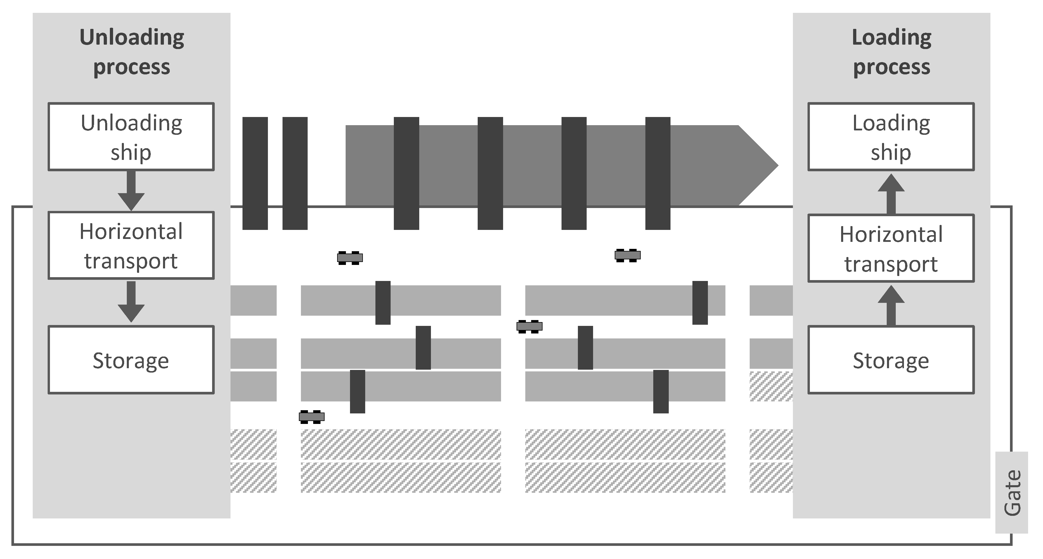
In the following, the created simulation model of the container terminal and its restrictions are presented. The discrete-event simulation model is implemented in Tecnomatix Plant Simulation and is based on the data of a real terminal. The layout of the terminal is shown in Figure 2.
The terminal has a quay length of 800 m and a total of 20 YBs. The simulation model represents container handling between the quayside and container yard. As displayed in Figure 2, the specifics of the design of the land-side transport interface as well as the berths are not considered in detail. In this study, parallel handling of several ships is not modeled. Consequently, the simulation model of the container terminal is stressed by the arrival of a single ship. For this, 12 bays of the ship with a total of 4000 containers have to be handled. About half of them are import containers to be unloaded and the other half are export containers to be loaded. The container transport orders are pre-defined and contain details such as the origin and destination of the containers at the terminal and the availability time for handling in the yard or quayside by gantry cranes. To reduce the execution time of a simulation run, three variations for each parameter combination are generated before all experiments. Depending on the experiment, at least 3 and at most 6 QCs are available for loading and unloading the ship. The ship is unloaded and loaded bay by bay, whereby the QC always handles the entire bay that is assigned to it. Thus, the QC moves after the unloading of a bay and before the loading of the next bay. These bay changes are represented by a delay between the handling of two containers of the same QC. When fewer QCs are used for one ship, more bays are served by each QC.
In the simulation model, an average quayside handling rate of 30 containers per hour is assumed, which is represented by an expected handling frequency of 120 s by each QC. To model stochastic influences, a triangular distribution of the QC handling times is assumed with a minimum handling time of 80 s and a maximum value of 180 s. YTs carry out horizontal transport between the quay and yard. Since YTs are unable to lift containers themselves, the transfer between the QC and YT must be synchronized. The travel times of the YTs are determined by the distances between QCs and YBs, as specified by the terminal layout. For calculating the travel times, an average speed of 8.4 m/s is assumed for the YTs. By inserting a triangular distribution, stochastic influences are taken into account when calculating the travel times. The total number of YTs used per experiment is generated in the yard at the beginning of the simulation.
The inbound and outbound yard operations are performed by RTGs. For the simulation model, it is assumed that RTGs can handle an average of 15 containers per hour, which corresponds to an expected value of 240 s per handling. Deviations and irregularities in the process are modeled by a triangular distribution with a minimum handling time of 180 s and a maximum value of 420 s. For all experiments, at least two YBs are required for each active QC. Thus, it can be ensured that sufficient stowage space is available for the containers to be handled. Depending on the experiment, one of the two storage policies random YB assignment and close YB assignment is investigated with the simulation model. For the storage policy random YB assignment, containers from all active YBs can be transported to and from each of the QCs. In addition, import containers are randomly assigned to YBs, regardless of which QC is used for the unloading. All active YBs are ensured to be equally burdened as much as possible. The second storage policy is close YB assignment, which seeks to minimize the distance between QCs and YBs. YBs with the shortest possible distance for horizontal transport are assigned to every QC. The handling of containers only takes place between the defined QCs and YBs.
Furthermore, the two different dispatching policies fixed QC-YT assignment and free QC-YT assignment are implemented in the simulation model. In the first policy, fixed QC-YT assignment, a fixed number of YTs are assigned to each QC. This policy is typically used in practical terminal operations, as it is the simplest to apply. Every YT receives an attribute that assigns it to a specific QC. In the second dispatching policy, free QC-YT assignment, each YT can approach every QC. This policy is a modified version of the hybrid method from Schwientek et al. [11]. The next suitable job is chosen on the basis of the necessary driving time at the terminal and the waiting time of orders. The driving time and waiting time can be weighted differently for each experiment, controlled by the policy tuning parameter Dispatching Weight. For the selection of the next suitable order, each free YT inspects the next 20 orders. The order with the earliest availability time is determined. For the other 19 orders, the difference between the order’s availability time and the earliest availability time is determined. Additionally, the required travel time to the start position of the respective order is calculated. Both values are multiplied by the intended weighting factor Dispatching Weight of the experiment. Finally, the results are added, and the order with the smallest sum is chosen by the YT. If no YT is available at the quay, the QCs have to wait. Otherwise, the containers can be loaded directly onto the YTs. Loaded YTs drive the containers to the defined YB. There, the YTs and containers are separated from each other. The same process steps for handling export containers occur in the reverse sequence of that described above.
2.2. Employed Meta-Heuristics
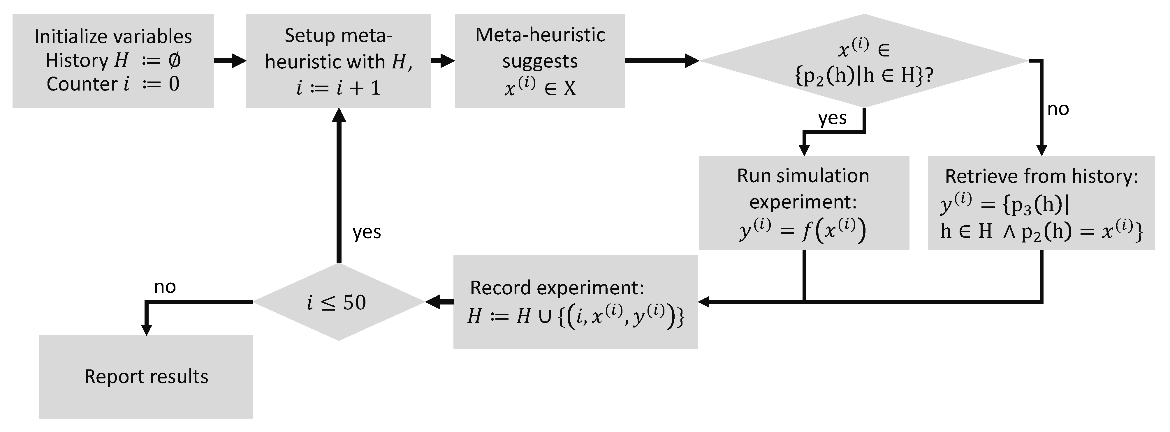
Meta-heuristics are used to approximate the best parameter configuration for the given simulation model described in the previous subsection. The corresponding process is depicted in Figure 3. First, the history H and the counter i are initialized as an empty set and 0, respectively. Since no prior observations are recorded in H, the meta-heuristic must select the experiment randomly. In the next step, the meta-heuristic suggests a parameter configuration . If this is a previously unseen parameter configuration, a simulation experiment is executed and the fitness is calculated. Otherwise, from the previous experiment runs stored in H, the fitness value corresponding to is retrieved. In both cases, H is extended with the new value, and the meta-heuristic is set up with this H. After 50 evaluations, the results are reported, and the optimization study is completed. The history H is implemented with a global database that shares the history over several optimization runs independently from the employed meta-heuristic during the retrieval phase, which helps to reduce the wall time. The meta-heuristic is only set up with experiments that are previously suggested within the same optimization run to ensure the independence of each optimization run for the subsequent evaluation.
Without having executed any simulation experiments, the simulation model must be considered a black-box. It is, therefore, impossible to know which of a set of given meta-heuristics would lead to the best approximation. Since many meta-heuristics themselves have a stochastic component, even two different optimization runs of the same meta-heuristic can result in different approximations of the optimum. Hence, for a yet unknown simulation model, it is unpredictable whether the optimum will be approximated sufficiently well and, if so, which meta-heuristic will achieve this. Each meta-heuristic needs to empirically prove its applicability to a problem [48]. In this study, TPE was applied to a discrete event simulation model and compared with SA, BO, and RS. These meta-heuristics are introduced next.
2.2.1. Tree-Structured Parzen Estimator
TPE was developed to automate the search for a sufficiently well-performing configuration of a Deep Belief Network [41]. For a Deep Belief Network, parameters are either categorical variables (e.g., the decision whether to use pre-processed or raw data) or continuous variables (e.g., the learning rate). Integer values can be modeled as either categorical variables (the numbers are mere labels) or continuous variables that are rounded before further use. In addition, dependencies between variables exist: One variable determines the number of network layers and then each layer is configured on its own. Having the configuration of the third layer as part of a parameter configuration is only reasonable if the variable encoding the number of layers is set to at least three. Such a parameter is called a conditional parameter. To reflect the dependencies, this type of parameter configuration space is adequately represented as a tree. This requires specific meta-heuristics that support such a tree structure. The TPE approach has produced good benchmark results [42,49], and the initial paper is among the most cited publications on hyper-parameter optimization; at the time of writing, Scopus indicates that there are 939 citations.
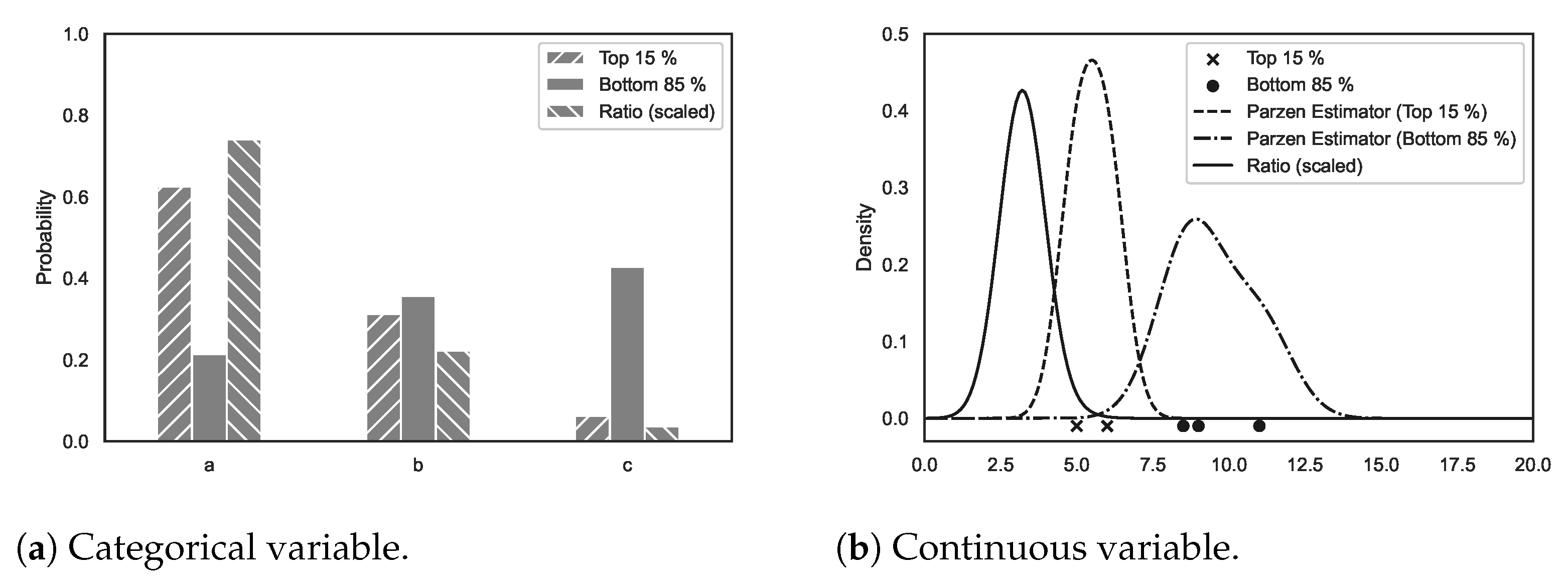
The TPE models , , and , where p denotes a probability density function (short: density), y is a point evaluation of the model, and x is a parameter configuration. The first density is a fixed value (e.g., 0.15 was used in the first publication) set by the experimenter, and is altered to fit the set value of for each iteration. The other two densities can be summarized as : The probability that a certain parameter configuration has been used, given a desired point evaluation value. Typically, TPE is formulated to find a minimum and, therefore, describes the density of parameters that have shown better results, whereas describes the density of the parameters that have led to poorer performance. As the true densities are unknown, they need to be estimated based on the obtained evaluations in each iteration. For each categorical parameter, two probability vectors are maintained and updated: Given the prior vector of probabilities , with each probability for representing one category, the posterior vector elements are proportional to , where counts the occurrences of choice i in the recorded evaluations so far. An example is depicted in Figure 4a. The estimator for the better-performing parameters (the top 15%) and that for the worse-performing parameters (the bottom 85%) are calculated based on the observations already recorded. For each continuous parameter, two adaptive Parzen estimators are used. Given a prior probability density distribution determined by the experimenter, with each point evaluation of the parameter configuration space with the help of the simulation model and the objective function, the densities are further approximated. An example is depicted in Figure 4b. The parameter choices of the better- and worse-performing models are used to create the respective densities. In each iteration, the model consisting of the two densities is used to select the next parameter configuration x to evaluate. To achieve this, several parameters x are sampled from the promising distribution . The parameter configuration x with the greatest expected improvement is chosen. This criterion is positively correlated with the ratio [41]. In Figure 4, this is referred to as ratio. The criterion favors the parameter configuration that has a high probability of leading to small evaluation values and a low probability of obtaining large evaluation values for the minimization problem at hand. After the parameter configuration has been evaluated by running the experiment and calculating the objective function value, the probability estimators are updated. For this publication, the reference implementation [49] in version 0.2.5 (the newest at the time of conducting the study), provided by the original authors, was chosen. As the prior distribution, a uniform distribution was chosen.
2.2.2. Simulated Annealing
SA is a meta-heuristic that is applicable to both combinatorial and multivariate problems [50], the latter of which is relevant for this optimization study. For this publication, the implementation of [49] in version 0.2.5 (the newest at the time of conducting the study) was used. This version of SA works on the tree structure presented in Figure 5. The tree structure requires some specific adjustments of the algorithm documented in [51]. The default initialization values of the implementation were used.
2.2.3. Bayesian Optimization
BO, also referred to as Gaussian process optimization, aims to minimize the expected deviation [52]. The response surface (i.e., the objective function values for given parameter configurations), including the uncertainty about the result, is estimated. For this publication, the implementation from [53] in version 1.2.6 (the newest at the time of conducting the study) was used. Since this procedure does not support tree-structured parameter configuration spaces, two simplifications are made. First, the numbers of YTs for the QC-YT Assignment fixed and free are grouped together. The parameter value ranges as in the right branch. If the fixed assignment is chosen, the number of YTs is divided by the number of QCs, and the result is rounded to the closest integer. Second, the dispatching weight is always set, even if it is not interpreted by the simulation model. During the initialization of an optimization run, five random experiments are conducted before BO takes over and guides the search.
2.2.4. Random Search
RS serves as a baseline. According to the NFLT, for some optimization problems, meta-heuristics perform worse than RS. It is crucial to identify meta-heuristics that misguide the search (e.g., by becoming stuck in local optima). For this publication, the implementation of [49] in version 0.2.5 (the newest at the time of conducting the study) was used, which is capable of sampling from a tree-structured parameter configuration space.
2.3. Optimization Procedure
The optimization procedure is written as an external program that encapsulates the simulation. First, the simulation model is initialized with the parameter configuration to examine. After the simulation runs for one experiment are finished, the output of the simulation model is read. The communication between the two programs is realized through the COM-Interface. The output values of the simulation model are inserted into the objective function, which determines the fitness of a given solution. This optimization procedure is described in more detail in the following.
2.3.1. Parameter Configuration Space
During initialization, each parameter of the parameter configuration is set as a global variable in the simulation model. The interpretation of one global variable in the simulation model can depend on another global variable. For example, the parameter #YTs is interpreted as the number of YTs for each QC for a fixed QC-YT assignment, but it is interpreted as the number of YTs for all QCs for a free QC-YT assignment. The parameter Dispatching Weight is the weight for the travel time and ranges from 0 to 1 in steps of . The weight for the availability time for handling is deduced by calculating 1. This parameter is only used for a free QC-YT assignment. Although setting this uninterpreted parameter does not harm the simulation experiment, the recorded observations for the meta-heuristic are flawed. This is because the meta-heuristic might use a record that includes the uninterpreted parameter to guide further search, despite the lack of any effect, which might guide the search process in the wrong direction.
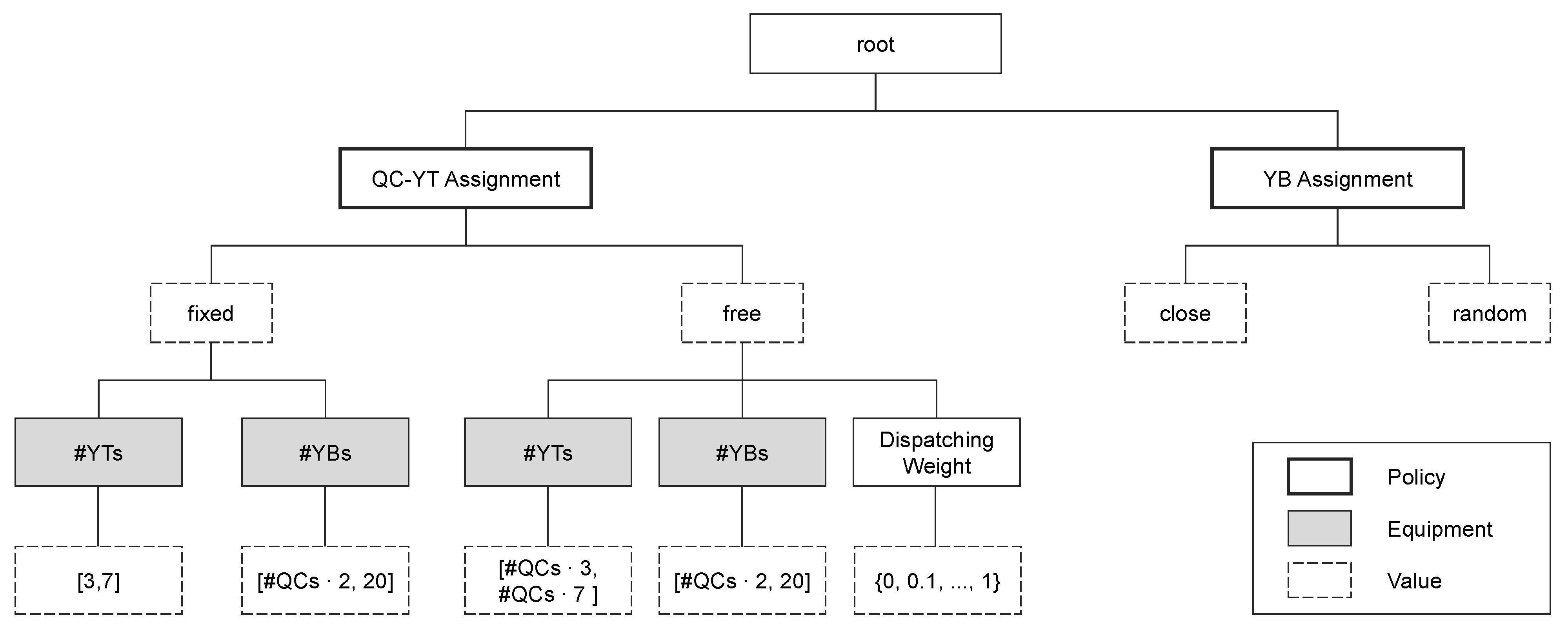
In Figure 5, the parameter configuration space is depicted in its tree form. It is dependent on the number of QCs, which can be either 3, 4, 5, or 6. Each case is considered to be independent and requires optimization.
The presented tree is used for TPE, SA, and RS. For BO, a vector representation is derived whereby each of the parameters QC-YT Assignment, YB Assignment, #YTs, #YBs, and Dispatching Weight are represented by one dimension of this vector. The different interpretation of #YTs is alleviated by varying the value over the range from #QCs · 3 to #QCs · 7 and, in the case of a fixed assignment, dividing by #QCs and then rounding that value to the closest integer value before using it to parameterize the simulation model. The parameter Dispatching Weight can theoretically take any value between 0 and 1. To make use of the caching mechanism, only steps of were permitted in this study.
2.3.2. Objective Function
After a simulation run is executed, the objective function is invoked to calculate the fitness for the given parameter configuration. The objective function needs to reflect the fact that the unloading and loading process needs to be fast, while at the same time, resources are only added if they are needed. Therefore, the following objective function was developed (based on [37]):
The left factor of the multiplication reflects the inverted relative makespan of the ship. is the time used to unload and load the ship. As an approximation of , prior to the optimization runs, 100 random samples are drawn from the parameter configuration space, and the makespan for the ship is measured. This normalization process centers the left factor to around 1 and ensures that it remains in proportion to the right factor. The shorter the makespan, the larger the left factor becomes.
The right factor of the multiplication is the weighted utilization. refers to the number of QCs, is the number of RTGs and, therefore, also the number of YBs, and is the number of trucks. refers to the ratio of the time for which the equipment has been working to the overall makespan. When summarizing these utilization values to one factor, weights are assigned according to the investment costs. It is assumed that a QC is 50 times more expensive than a truck, and the cost of an RTG is 10% of a QC [37]. The higher the equipment utilization (with a special focus on expensive equipment), the larger the right factor becomes.
2.3.3. Structure of Optimization Study
For each scenario (3, 4, 5, and 6 QCs) and meta-heuristic (TPE, BO, SA, and RS), 50 optimization runs are executed. This allows for gaining insights on the reproducibility of the optimization results using meta-heuristics. Each optimization run consists of 50 experiments. For each experiment, 30 simulation runs are executed. The results of each simulation run vary slightly due to stochastic factors. These are implemented by drawing handling times from random distributions, as described in Section 2.1.
3. Results and Discussion
In the following, the experimental results of the optimization study are analyzed. Then, the solutions found for the different meta-heuristics are compared and discussed.
3.1. Preparatory Study
The objective function (see Equation (1)) requires , the median of . The population parameter is only known after exhaustive coverage of the parameter configuration space, which must be avoided for an optimization study. As a replacement, a sample estimate must suffice. For this purpose, for each scenario, 100 parameter configurations were sampled randomly, and the corresponding simulation experiments were run. For each of these simulation experiments, the makespan of the ship was recorded. The median, minimum, and maximum of the makespan are noted in Table 1. The values in the median column are used as for the respective scenario.
Table 1 shows that the median and minimum both decrease as the number of QCs increases. The median shows that using 4 QCs instead of 3 results in a reduction of ca. 20% in the makespan. By doubling the number of QCs from 3 to 6, the performance can be increased by ca. 57%. This is not true for the maximum, which remains nearly constant at around 160 h. Furthermore, the difference between 4 and 5 QCs is rather small. This can be explained by the fact that in the simulation model, 12 bays of the ship are handled. With 4 QCs, each QC handles exactly 3 bays. With 5 QCs, 3 QCs are responsible for 2 bays each, and 2 QCs are responsible for 3 bays each. Thus, 3 QCs complete the container handling task earlier, but the makespan is based on the QC that finishes last.
3.2. Observations from All Experiments
In the scope of the optimization study, 40,000 experiments in total were evaluated. For each scenario (3, 4, 5, and 6 QCs) and each meta-heuristic (TPE, BO, SA, and RS), 50 optimization runs were executed, each consisting of 50 experiments. This set of experiments covers many randomly chosen experiments (e.g., RS or initialization phase of any of the meta-heuristics) in addition to experiments that are biased by the manner in which each meta-heuristic works during its search process. This overview, which omits the search process, provides some insights into the characteristics of the simulation model.
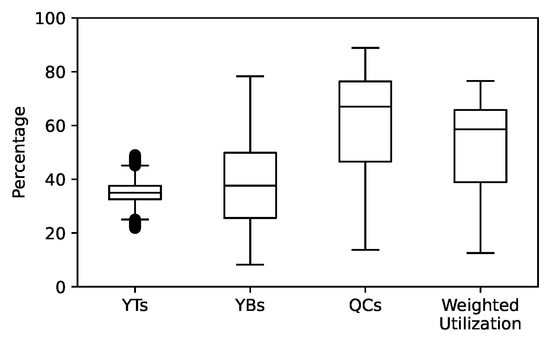
For each experiment, among others, the makespan, as well as the utilization of the equipment, is measured. The utilization is the arithmetic mean of the working time of all equipment of its respective type. In Figure 6, the utilization of YTs, YBs, and QCs is shown. Due to the larger investment costs, the weighted utilization is closest to the QCs. The median of the utilization of the YTs is the lowest. Since a YT cannot lift a container itself, it must wait for a gantry crane (either QC or RTG) to load or unload the YT. High utilization of QCs and YBs is only possible if enough YTs are available, which inevitably results in lower utilization on the YT side. As the utilization of YTs is assigned a rather small weight in the fitness function, the lower utilization rate carries no relevant weight.
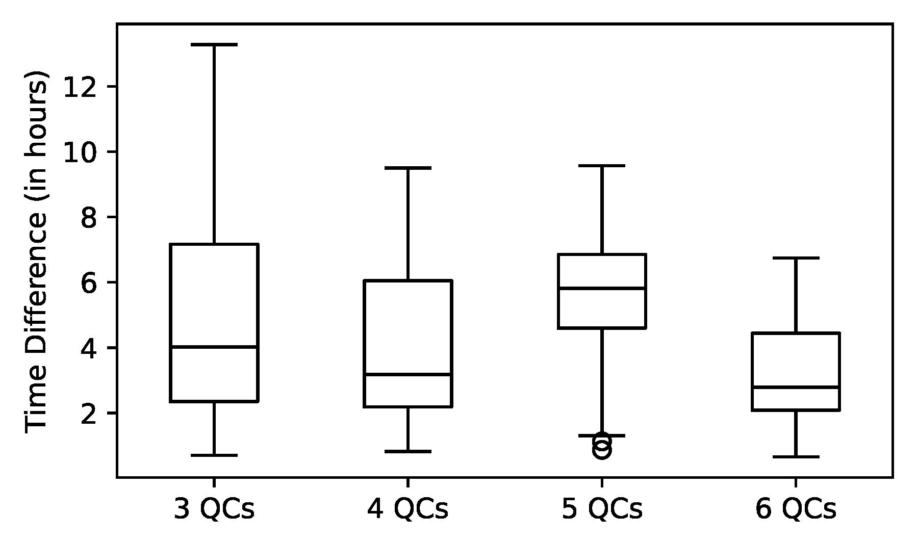
In Figure 7, the difference between the maximum and minimum working times of the YTs for each experiment that used the global assignment policy is depicted. This is an indicator of how effectively the work is shared among YTs. As a general tendency, it can be seen that more QCs lead to less statistical scattering.
3.3. Approximated Optima
Both the preparatory study and the first screening of all executed experiments created first impressions of the underlying processes. Within the parameter configuration tree, there are exceptionally low-performing solutions. This raises the following question: Which of the meta-heuristics identified the best parameter configuration? To determine this, for each optimization run, the experiment with the highest fitness is extracted. During optimization, both TPE and BO select the next experiment with the greatest expected improvement. Hence, in contrast to SA, after a phase of exploitation (i.e., minor adjustments), a phase of exploration (i.e., larger changes) can follow. RS is the most extreme example since exploitation is never sought. This, in turn, means that the best result of an optimization run can appear at any position of the sequence of recorded experiments.
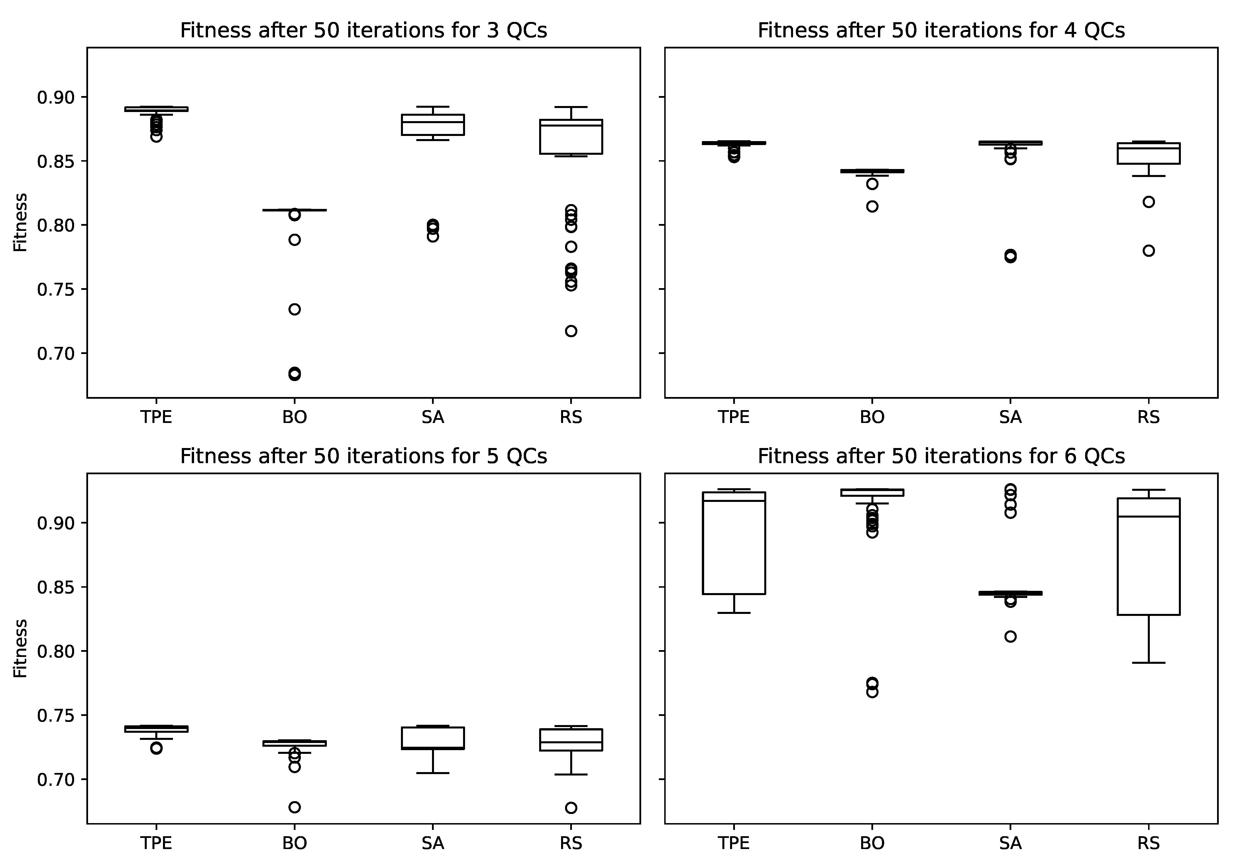
In Figure 8, the four meta-heuristics TPE, BO, SA, and RS are compared for each scenario with 3, 4, 5, and 6 QCs. Consistent with the preparatory study, the results for 5 QCs are far worse than those of all other scenarios. Each of the meta-heuristics shows outliers in at least three of the boxplots, which indicates the importance of stochastic influences during the search process. There is no clear ranking among the meta-heuristics. For 3 QCs, BO performs considerably worse than the other three meta-heuristics. These results are similar for 4 and 5 QCs, although with less severity. This is especially interesting since, for 6 QCs, BO produces the highest median. Over the first three scenarios, RS and SA have very similar performances, and for 6 QCs, SA has the worst median, with outliers in both directions. TPE performs very well in the first three scenarios, providing many of the best solutions with few outliers that are substantially worse. For 6 QCs, the median of TPE is much lower than that of BO. However, in two instances, BO arrived at substantially lower-performing solutions.
The differences between meta-heuristics were examined statistically. A significance level of was chosen for the whole study and corrected for each test using Bonferroni correction. To make general statements regarding the meta-heuristics, all scenarios (different numbers of QCs) are agglomerated. The large number of outliers for some of the meta-heuristics precludes the assumption of a normal distribution and requires a nonparametric approach. Hence, a Kruskal–Wallis H test was employed. The test statistic of leads to . Hence, the null hypothesis that the four groups stem from a single population is rejected. In a posthoc Nemenyi’s test for pairwise comparison, only TPE was significantly different from the other meta-heuristics. In other words, BO and SA are not significantly different from RS. The comparison of descriptive statistics (as the reader can approximate from Figure 8) shows the superiority of TPE in this study.
The wide range of approximated optima and the large difference between meta-heuristics are indicators of the complexity of the simulation model. The parameter configurations of all optima are more closely examined in the following. The meta-heuristics always determine that the fixed assignment of YTs to QCs leads to an inferior performance compared with pooling. Furthermore, in all instances, the pairing of each QC with its closest YBs performs better than delivering each container to a randomly chosen YB. In contrast to these parameters, the parameter Dispatching Weight shows no clear interpretable results.
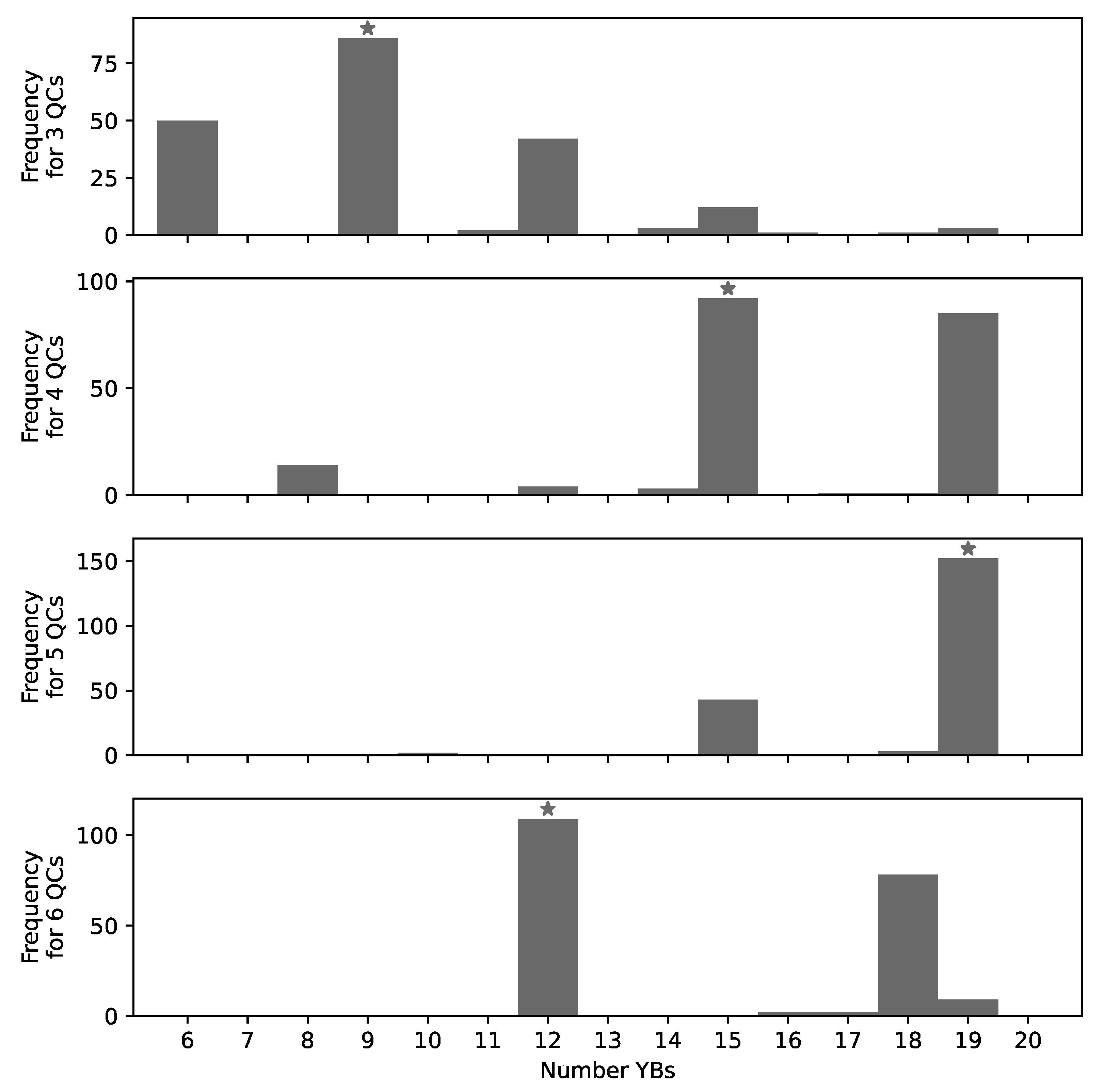
In Figure 9, the frequencies of specific numbers of YBs for 3, 4, 5, and 6 QCs are depicted. A small number of YBs creates a bottleneck in the yard, while having too many YBs leads to a low utilization of each YB as well as longer travel paths of the YTs. The fewer YBs are used, the shorter the traveled paths, the higher the probability that an unloading job and a loading job can be combined. The number of used YBs is often a multiple of the number of QCs. This can be explained by the rather conservative transportation job assignment policy in place, which is designed to avoid traffic jams but rather postpones a job.
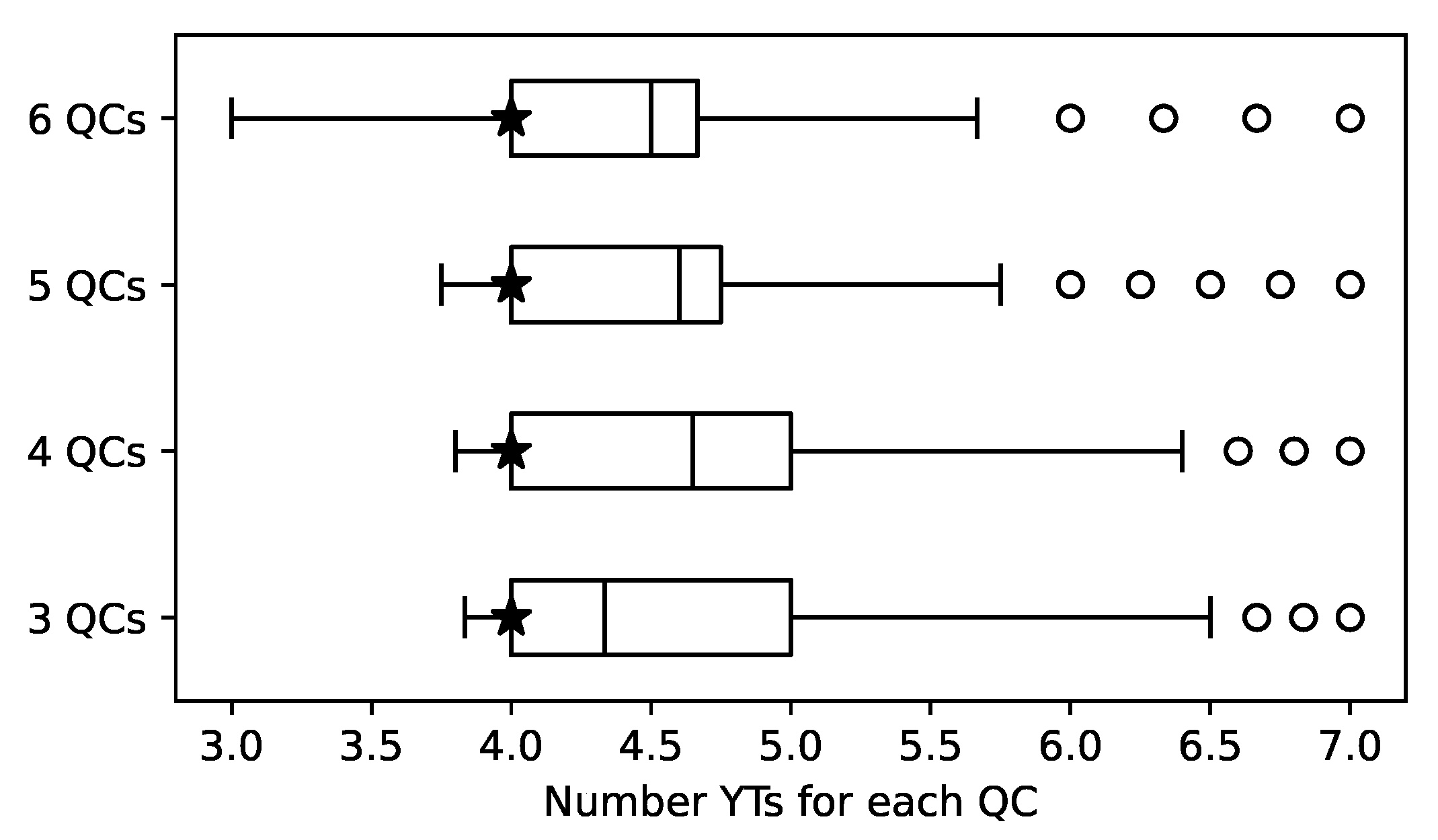
In Figure 10, the number of YTs per QC for each scenario is presented. The large number of outliers to the right can be explained by the rather small impact of the number of trucks on the weighted utilization and, therefore, on the objective function.
In this study, as in [24], TPE exhibits the most robust behavior. Of the 200 optimization runs, TPE never returns the worst approximation of the optimum. For some scenarios, other meta-heuristics provide better medians of approximations. At the same time, only TPE is significantly different from RS when the data are agglomerated over all scenarios. These observations provide evidence that TPE is an appropriate approach. For an explicit recommendation, meta-analyses of several publications using the same meta-heuristics are required in future to accumulate such evidence.
In comparison with [37], this study shows an alternative approach to calibrating the quantity of equipment used in different functional areas of a container terminal. In addition, policies are selected and tuned (if the policy accepts a parameter). The approach of Kotachi et al. [37] requires all parameters to be at least on an ordinal scale since the mutation is defined as changing a parameter one level up or down. For categorical parameters that can take more than two values, there is no order. For continuous parameters, this mutation makes it necessary to define a step size. The approach presented in this study also discretizes the parameter Dispatching Weight to the the set . However, this is performed to enable caching to speed up the optimization study. All of the meta-heuristics used support continuous parameters, which might be of interest for future optimization studies.
4. Conclusions
This study provides an approach to solving integrated decision problems at container terminals. Earlier studies have often approached such problems by using a mathematical model that aims to optimize the schedule of jobs. Depending on the concept, sometimes the schedule is determined hours before the actual execution of a job, which is an appropriate approach in rather deterministic environments. Another common approach in the literature is to define a policy that is evaluated using a simulation study. The design of experiments—e.g., a full-factorial design with a coarse grid—leads to either very large simulation studies or a selection of experiments biased by the researcher’s beliefs. These shortcomings of optimization alone and manually designed large simulation studies are partly overcome by the presented simulation-based optimization approach. This approach uses simulation to evaluate the quality of a given solution, and only in this way can the dynamics of real systems be properly represented. Simulation-based optimization allows for the possibility of illustrating these dynamics, providing an approximated solution to the problem without maintaining a separate mathematical model. Therefore, further decision problems can be integrated into the simulation model and the parameter configuration space with little effort.
The authors showed the transferability of meta-heuristics, which originate from the domain of machine learning or have been successfully applied in that area. These methods could be used to optimize discrete event simulation models. A special focus was placed on discrete and continuous parameters that were potentially interdependent. Several optimization runs guided by different meta-heuristics were executed and with a restricted computational budget, promising parameter configuration ranges were identified. This publication focused on examining the results of different optimization runs. For this purpose, the numbers of QCs, YTs, and YBs were modified during different experiments. At the same time, different dispatching policies, as well as QC-YB assignment policies, were investigated. Furthermore, different allocation policies of YBs were applied. In this study, the approximated optima suggest that the pooling of YTs was preferable to free allocation. Furthermore, a YB assignment close to the QCs was considered better than a random one. By choosing more QCs, the number of bays to be served per QC decreased. Thus, a reduction of the makespan could be achieved. A doubling of the number of QCs from 3 to 6 led to a reduction of the makespan by 57%.
Due to the NFLT, it is not clear whether these empirical results can be generalized to future studies that use simulation-based optimization. The applicability of meta-heuristics such as TPE or BO needs to be demonstrated by further optimization studies, potentially with various simulation models, different objective functions, and additional meta-heuristics or different fine-tuning of the same meta-heuristic for comparison.
Author Contributions
Conceptualization, M.K., A.S., C.J., and N.N.; methodology, M.K., A.S., and N.N.; software, M.K., A.S., and N.N.; validation, M.K.; formal analysis, M.K.; investigation, N.N., M.K.; resources, N.N.; data curation, M.K.; writing—original draft preparation, M.K., A.S., and N.N.; writing—review and editing, A.S., C.J.; visualization, N.N., M.K.; supervision, C.J.; project administration, M.K. All authors have read and agreed to the published version of the manuscript.
Funding
This research received no external funding.
Data Availability Statement
The data presented in this study are openly available in zenodo at 10.5281/zenodo.4473251.
Conflicts of Interest
The authors declare no conflict of interest.
Abbreviations
The following abbreviations are used in this manuscript:
| BO | Bayesian Optimization |
| NFLT | No Free Lunch Theorem |
| QC | Quay Crane |
| RS | Random Search |
| RTG | Rubber-tired Gantry Crane |
| SA | Simulated Annealing |
| TPE | Tree-structured Parzen Estimator |
| TEU | Twenty-foot Equivalent Unit |
| YB | Yard Block |
| YT | Yard Truck |
References
- UNCTAD. Review of Maritime Transport; United Nations: New York, NY, USA, 2020. [Google Scholar]
- Karam, A.; Eltawil, A.; Harraz, N. Simultaneous assignment of quay cranes and internal trucks in container terminals. Int. J. Ind. Syst. Eng. 2016, 24, 107–125. [Google Scholar] [CrossRef]
- Gharehgozli, A.; Zaerpour, N.; de Koster, R. Container terminal layout design: Transition and future. Marit. Econ. Logist. 2020, 22, 610–639. [Google Scholar] [CrossRef]
- Bierwirth, C.; Meisel, F. A follow-up survey of berth allocation and quay crane scheduling problems in container terminals. Eur. J. Oper. Res. 2015, 244, 675–689. [Google Scholar] [CrossRef]
- Kizilay, D.; Eliiyi, D.T. A comprehensive review of quay crane scheduling, yard operations and integrations thereof in container terminals. Flex. Serv. Manuf. J. 2020, 1, 1–42. [Google Scholar] [CrossRef]
- Chen, L.; Langevin, A.; Lu, Z. Integrated scheduling of crane handling and truck transportation in a maritime container terminal. Eur. J. Oper. Res. 2013, 225, 142–152. [Google Scholar] [CrossRef]
- Lange, A.K.; Schwientek, A.K.; Jahn, C. Reducing truck congestion at ports—Classification and trends. Digitalization in Maritime and Sustainable Logistics. In Proceedings of the Hamburg International Conference of Logistics (HICL); Jahn, C., Kersten, W., Ringle, C.M., Eds.; Epubli: Berlin, Germany, 2017; pp. 37–58. [Google Scholar]
- Cordeau, J.F.; Legato, P.; Mazza, R.M.; Trunfio, R. Simulation-based optimization for housekeeping in a container transshipment terminal. Comput. Oper. Res. 2015, 53, 81–95. [Google Scholar] [CrossRef]
- Dragovic, B.; Tzannatos, E.; Park, N.K. Simulation modelling in ports and container terminals: Literature overview and analysis by research field, application area and tool. Flex. Serv. Manuf. J. 2017, 29, 4–34. [Google Scholar] [CrossRef]
- Angeloudis, P.; Bell, M.G. A review of container terminal simulation models. Marit. Policy Manag. 2011, 38, 523–540. [Google Scholar] [CrossRef]
- Schwientek, A.K.; Lange, A.K.; Jahn, C. Effects of terminal size, yard block assignment, and dispatching methods on container terminal performance. In Winter Simulation Conference 2020; Bae, K.H., Feng, B., Kim, S., Zheng, Z., Roeder, T., Thiesing, R., Eds.; IEEE Press: New York, NY, USA, 2020. [Google Scholar]
- Zhen, L.; Yu, S.; Wang, S.; Sun, Z. Scheduling quay cranes and yard trucks for unloading operations in container ports. Ann. Oper. Res. 2016, 122, 21. [Google Scholar] [CrossRef]
- He, J.; Huang, Y.; Yan, W.; Wang, S. Integrated internal truck, yard crane and quay crane scheduling in a container terminal considering energy consumption. Expert Syst. Appl. 2015, 42, 2464–2487. [Google Scholar] [CrossRef]
- Cao, P.; Jiang, G.; Huang, S.; Ma, L. Integrated simulation and optimisation of scheduling yard crane and yard truck in loading operation. Int. J. Shipp. Transp. Logist. 2020, 12, 230–250. [Google Scholar] [CrossRef]
- Castilla-Rodríguez, I.; Expósito-Izquierdo, C.; Melián-Batista, B.; Aguilar, R.M.; Moreno-Vega, J.M. Simulation-optimization for the management of the transshipment operations at maritime container terminals. Expert Syst. Appl. 2020, 139, 112852. [Google Scholar] [CrossRef]
- Kizilay, D.; Eliiyi, D.T.; van Hentenryck, P. Constraint and mathematical programming models for integrated port container terminal operations. Integration of Constraint Programming, Artificial Intelligence, and Operations Research. Lect. Notes Comput. Sci. 2018, 10848, 344–360. [Google Scholar] [CrossRef] [Green Version]
- Karam, A.; Eltawil, A.; Hegner Reinau, K. Energy-Efficient and Integrated Allocation of Berths, Quay Cranes, and Internal Trucks in Container Terminals. Sustainability 2020, 12, 3202. [Google Scholar] [CrossRef] [Green Version]
- Karam, A.; Eltawil, A. Functional integration approach for the berth allocation, quay crane assignment and specific quay crane assignment problems. Comput. Ind. Eng. 2016, 102, 458–466. [Google Scholar] [CrossRef]
- Sislioglu, M.; Celik, M.; Ozkaynak, S. A simulation model proposal to improve the productivity of container terminal operations through investment alternatives. Marit. Policy Manag. 2019, 46, 156–177. [Google Scholar] [CrossRef]
- Muravev, D.; Rakhmangulov, A.; Hu, H.; Zhou, H. The introduction to system dynamics approach to operational efficiency and sustainability of dry port’s main parameters. Sustainability 2019, 11, 2413. [Google Scholar] [CrossRef] [Green Version]
- Muravev, D.; Hu, H.; Rakhmangulov, A.; Mishkurov, P. Multi-agent optimization of the intermodal terminal main parameters by using AnyLogic simulation platform: Case study on the Ningbo-Zhoushan Port. Int. J. Inf. Manag. 2020, 1, 102133. [Google Scholar] [CrossRef]
- Kastner, M.; Pache, H.; Jahn, C. Simulation-based optimization at container terminals: A literature review. In Digital Transformation in Maritime and City Logistics, Proceedings of the Hamburg International Conference of Logistics (HICL); Jahn, C., Kersten, W., Ringle, C.M., Eds.; Epubli GmbH: Berlin, Germany, 2019; pp. 111–135. [Google Scholar] [CrossRef]
- Zhou, C.; Li, H.; Liu, W.; Stephen, A.; Lee, L.H.; Peng Chew, E. Challenges and opportunities in integration of simulation and optimization in maritime logistics. In Proceedings of the 2018 Winter Simulation Conference, Gothenburg, Sweden, 9–12 December 2018; pp. 2897–2908. [Google Scholar] [CrossRef]
- Kastner, M.; Nellen, N.; Jahn, C. Model-based optimisation with tree-structured parzen estimation for container terminals. In ASIM 2019 Simulation in Produktion und Logistik 2019; Putz, M., Schlegel, A., Eds.; Wissenschaftliche Scripten: Auerbach, Germany, 2019; pp. 489–498. [Google Scholar]
- Singgih, I.K.; Jin, X.; Hong, S.; Kim, K.H. Architectural design of terminal operating system for a container terminal based on a new concept. Ind. Eng. Manag. Syst. 2016, 15, 278–288. [Google Scholar] [CrossRef] [Green Version]
- Schwientek, A. Abilities of the Used Terminal Operating Systems: Personal Conversation, 2012–2013.
- Barton, R.R. Simulation experiment design. In Proceedings of the 2010 Winter Simulation Conference, Piscataway, NJ, USA, 5–8 December 2010; pp. 75–86. [Google Scholar] [CrossRef] [Green Version]
- Li, H.; Zhou, C.; Lee, B.K.; Lee, L.H.; Chew, E.P.; Goh, R.S.M. Capacity planning for mega container terminals with multi-objective and multi-fidelity simulation optimization. IISE Trans. 2017, 49, 849–862. [Google Scholar] [CrossRef]
- Al-Salem, M.; Almomani, M.; Alrefaei, M.; Diabat, A. On the optimal computing budget allocation problem for large scale simulation optimization. Simul. Model. Pract. Theory 2017, 71, 149–159. [Google Scholar] [CrossRef]
- Ho, Y.C.; Zhao, Q.C.; Jia, Q.S. (Eds.) Ordinal Optimization: Soft Optimization for Hard Problems; Springer: New York, NY, USA, 2007. [Google Scholar]
- Xu, J.; Huang, E.; Chen, C.H.; Lee, L.H. Simulation optimization: A review and exploration in the new era of cloud computing and big data. Asia-Pac. J. Oper. Res. 2015, 32, 1–34. [Google Scholar] [CrossRef]
- Fu, M.C.; Glover, F.W.; April, J. Simulation optimization: A review, new developments, and applications. In Proceedings of the 2005 Winter Simulation Conference, Orlando, FL, USA, 4–7 December 2005; pp. 351–380. [Google Scholar]
- Figueira, G.; Almada-Lobo, B. Hybrid simulation–optimization methods: A taxonomy and discussion. Simul. Model. Pract. Theory 2014, 46, 118–134. [Google Scholar] [CrossRef] [Green Version]
- Hanschke, T.; Krug, W.; Nickel, S.; Zisgen, H. VDI 3633 Blatt 12 - Simulation und Optimierung. In VDI-Handbuch Fabrikplanung und -Betrieb-Band 2: Modellierung und SIMULATION; Beuth: Berlin, Germany, 2016. [Google Scholar]
- Juan, A.A.; Faulin, J.; Grasman, S.E.; Rabe, M.; Figueira, G. A review of simheuristics: Extending metaheuristics to deal with stochastic combinatorial optimization problems. Oper. Res. Perspect. 2015, 2, 62–72. [Google Scholar] [CrossRef] [Green Version]
- Chopard, B.; Tomassini, M. An Introduction to Metaheuristics for Optimization, 1st ed.; Natural Computing Series; Springer International Publishing: Cham, Switzerland, 2018. [Google Scholar]
- Kotachi, M.; Rabadi, G.; Seck, M.; Msakni, M.K.; Al-Salem, M.; Diabat, A. Sequence-based simulation optimization: An application to container terminals. In Proceedings of the 2018 IEEE Technology & Engineering Management Conference, Piscataway, NJ, USA, 27 June–1 July 2018; pp. 1–7. [Google Scholar] [CrossRef]
- Géron, A. Hands-on Machine Learning with Scikit-Learn, Keras, and TensorFlow: Concepts, Tools, and Techniques to Build Intelligent Systems, 2nd ed.; O’Reilly UK Ltd.: Newton, MA, USA, 2019. [Google Scholar]
- Bergstra, J.; Bengio, Y. Random search for hyper-parameter optimization. J. Mach. Learn. Res. 2012, 13, 281–305. [Google Scholar]
- Hutter, F.; Hoos, H.H.; Leyton-Brown, K. Sequential model-based optimization for general algorithm configuration. In Learning and Intelligent Optimization; Coello, C.A.C., Ed.; Springer: Berlin/Heidelberg, Germany, 2011; pp. 507–523. [Google Scholar]
- Bergstra, J.; Bardenet, R.; Bengio, Y.; Kégl, B. Algorithms for hyper-parameter optimization. In Proceedings of the 25th Annual Conference on Neural Information Processing Systems, Granada, Spain, 12–14 December 2011; Volume 24, pp. 2546–2554. [Google Scholar]
- Eggensperger, K.; Feurer, M.; Hutter, F.; Bergstra, J.; Snoek, J.; Hoos, H.; Leyton-Brown, K. Towards an empirical foundation for assessing Bayesian optimization of hyperparameters. In Proceedings of the NIPS Workshop on Bayesian Optimization in Theory and Practice, Lake Tahoe, NV, USA, 10 December 2013; pp. 1–5. [Google Scholar]
- Madrigal, F.; Maurice, C.; Lerasle, F. Hyper-parameter optimization tools comparison for multiple object tracking applications. Mach. Vis. Appl. 2019, 30, 269–289. [Google Scholar] [CrossRef] [Green Version]
- Yang, L.; Shami, A. On hyperparameter optimization of machine learning algorithms: Theory and practice. Neurocomputing 2020, 415, 295–316. [Google Scholar] [CrossRef]
- Gijsbers, P.; LeDell, E.; Poirier, S.; Thomas, J.; Bischl, B.; Vanschoren, J. An open source AutoML benchmark. In Proceedings of the 6th ICML Workshop on Automated Machine Learning, Long Beach, CA, USA, 14–15 June 2019. [Google Scholar]
- Akiba, T.; Sano, S.; Yanase, T.; Ohta, T.; Koyama, M. Optuna: A next-generation hyperparameter optimization framework. In Proceedings of the 25th ACM SIGKDD International Conference on Knowledge Discovery & Data Mining, Anchorage, AK, USA, 4–8 August 2019; pp. 2623–2631. [Google Scholar] [CrossRef]
- Wolpert, D.H.; Macready, W.G. No free lunch theorems for optimization. IEEE Trans. Evol. Comput. 1997, 1, 67–82. [Google Scholar] [CrossRef] [Green Version]
- McDermott, J. When and why metaheuristics researchers can ignore “No Free Lunch” theorems. Metaheuristics 2019, 1, 67. [Google Scholar] [CrossRef]
- Bergstra, J.; Yamins, D.; Cox, D.D. Making a science of model search: Hyperparameter optimization in hundreds of dimensions for vision architectures. In Proceedings of the 30th International Conference on Machine Learning, Atlanta, GA, USA, 16–21 June 2013; pp. 115–123. [Google Scholar]
- Kirkpatrick, S.; Gelatt, C.D.; Vecchi, M.P. Optimization by simulated annealing. Science 1983, 220, 671–680. [Google Scholar] [CrossRef]
- Bergstra, J. Simulated Annealing. Available online: https://github.com/hyperopt/hyperopt/blob/master/hyperopt/anneal.py (accessed on 29 December 2020).
- Močkus, J. On Bayesian methods for seeking the extremum. In Optimization Techniques IFIP Technical Conference; Springer: Berlin/Heidelberg, Germany, 1975; pp. 400–404. [Google Scholar]
- The GPyOpt Authors. GPyOpt: A Bayesian Optimization Framework in Python. Available online: http://github.com/SheffieldML/GPyOpt (accessed on 29 December 2020).
Figure 1.
Decision problems at container terminals.

Figure 2.
Layout and process illustration of the simulation model.

Figure 3.
The optimization process.

Figure 4.
The Tree-structured Parzen Estimation (TPE) uses the ratio of better- and worse-performing parameters to guide the search. In the example on the left, the categorical variable takes one of the three values “a”, “b”, and “c”. For the continuous variable, in the example on the right the values range from 0 to 20.

Figure 5.
The parameter configuration space in tree form.

Figure 6.
The utilization of the equipment over all experiments.

Figure 7.
Time difference between maximum and minimum working times of YTs.

Figure 8.
The approximated optima for each scenario and each meta-heuristic.

Figure 9.
The number of YBs in the set of approximated optima. The parameter value that leads to the best objective function value over all optimization runs is marked with an asterisk.
Figure 9.
The number of YBs in the set of approximated optima. The parameter value that leads to the best objective function value over all optimization runs is marked with an asterisk.

Figure 10.
The number of YTs in the set of approximated optima. The parameter value that leads to the best objective function value over all optimization runs is marked with an asterisk.
Figure 10.
The number of YTs in the set of approximated optima. The parameter value that leads to the best objective function value over all optimization runs is marked with an asterisk.


Table 1.
Makespan of the ship for 100 randomly drawn experiments.
| Number of QCs | Makespan (in Hours, Rounded) | ||
|---|---|---|---|
| Median | Minimum | Maximum | |
| 3 | 61 | 51 | 158 |
| 4 | 49 | 39 | 161 |
| 5 | 47 | 38 | 160 |
| 6 | 35 | 29 | 161 |
Publisher’s Note: MDPI stays neutral with regard to jurisdictional claims in published maps and institutional affiliations. |
© 2021 by the authors. Licensee MDPI, Basel, Switzerland. This article is an open access article distributed under the terms and conditions of the Creative Commons Attribution (CC BY) license (http://creativecommons.org/licenses/by/4.0/).
Share and Cite
MDPI and ACS Style
Kastner, M.; Nellen, N.; Schwientek, A.; Jahn, C. Integrated Simulation-Based Optimization of Operational Decisions at Container Terminals. Algorithms 2021, 14, 42. https://0-doi-org.brum.beds.ac.uk/10.3390/a14020042
AMA Style
Kastner M, Nellen N, Schwientek A, Jahn C. Integrated Simulation-Based Optimization of Operational Decisions at Container Terminals. Algorithms. 2021; 14(2):42. https://0-doi-org.brum.beds.ac.uk/10.3390/a14020042
Chicago/Turabian StyleKastner, Marvin, Nicole Nellen, Anne Schwientek, and Carlos Jahn. 2021. "Integrated Simulation-Based Optimization of Operational Decisions at Container Terminals" Algorithms 14, no. 2: 42. https://0-doi-org.brum.beds.ac.uk/10.3390/a14020042
Note that from the first issue of 2016, this journal uses article numbers instead of page numbers. See further details here.