Article

Number of Financial Indicators as a Factor of Multi-Criteria Analysis via the TOPSIS Technique: A Municipal Case Study

1
Department of Public Economics, Faculty of Economics, VŠB—Technical University of Ostrava, Sokolská třída 33, 70200 Ostrava, Czech Republic
2
Faculty of Natural Sciences, Institute of Economics and Management, Constantine the Philosopher University in Nitra, Trieda Andreja Hlinku 1, 94974 Nitra, Slovakia
3
Department of Regional Economics and Administration, Faculty of Economics and Administration, Masaryk University, Lipová 41a, 60200 Brno, Czech Republic
4
Department of Corporate Economics and Management, Faculty of Economics, Matej Bel University in Banská Bystrica, Tajovského 10, 97590 Banská Bystrica, Slovakia
5
Department of Tourism and Hotel Management, Faculty of Management, University of Prešov, Konštantínova 16, 08001 Prešov, Slovakia
*
Author to whom correspondence should be addressed.
Submission received: 19 January 2021 / Revised: 16 February 2021 / Accepted: 17 February 2021 / Published: 19 February 2021
(This article belongs to the Special Issue Algorithms and Models for Dynamic Multiple Criteria Decision Making)

Abstract

:
Multi-criteria analysis is a decision-making and efficiency assessment tool for application in both the private and public sectors. Its application is preceded by the selection of suitable indicators and a homogenous set of variants, as well as suitable methods based on the nature of the input data. The goal of the submitted research is to highlight the importance of selecting suitable indicators using a case study assessment of the financial health of a municipality—more precisely, the efficiency of management of this municipality. Four key indicators, thirty-two homogenous subjects, and one multi-criteria analysis method were identified in this study based on the theoretical foundations of the specific issue. These elements were processed into a total of 14 variants depending on the number of assessed indicators. Then, these results were subjected to statistical verification alongside verification using the Jaccard index. Based on the acquired results, we highlight the need for correct and expert identification of the relevant sets of alternatives (the criteria matrix) and expert discussion, which should precede the selection of the assessed indicators and objectify this selection process as much as possible. Assessment based on a low number of indicators was shown to be insufficient, highly variable, and diverse, and these differences were partially eliminated as the number of assessed indicators increased.

1. Introduction

Application of financial analysis methods in the field of local government has become increasingly important in recent years and also increasingly used in practice. Successful financial management creates the basis for long-term financial stability, increased competitiveness, increased performance of individual financial goals, achievement of the optimal formation of a monetary base, allocation of that monetary base to asset folders, and resulting effects from the specific activity [1]. Consequently, the importance of financial analysis is increasing in business activities. Some authors [2,3,4,5,6] believe that managerial decisions made in local government and non-profit organisations are not significantly different from managerial decisions made within companies. Therefore, the use of individual methods can be observed across the private and public sector.
Each of these methods works with several different indicators. Therefore, our main research question is as follows: How many (financial) criteria are enough—one, two, or more? The main goal of this paper is to highlight the importance of selecting suitable indicators based on a case study assessment of the financial health of municipalities, as well as the effectiveness of the management of those indicators, which directly determines the results of the entire assessment. For this study, three specific goals were defined. We maintain that the main problem is the correct selection of evaluation indicators, which directly determine the results of the entire assessment and are often given insufficient attention.
In the first section, we focus on the importance and need for financial analysis in the 21st century and identify the methods applied in the field of public administration and local government. The second section contains a description of the presented concept in the form of a methodology, which is devoted to the importance of homogenous research samples and the subsequent selection of assessment indicators for the assessment of local government subjects, i.e., municipalities. The importance of correctly selecting these indicators is illustrated in the third section, which gives the results of the assessment of municipalities, utilising various arrangements of the monitored indicators (a total of 14 executed variants) and assessment of those indicators based on the coincidence of the acquired results. The last section is the conclusion, where our results are interpreted in the context of research by other authors, and the conclusions from our own research are outlined.

2. Theoretical Background

Financial analysis is an important part of the financial management of an organisation. Financial analysis is implicitly assumed to be used in the private sector, which does not preclude its further application to the public sector when making economic decisions. Using a thoroughly executed financial analysis, individual subjects are capable of identifying the causes of occurring deviations [7], which may have a positive or negative character. Financial analysis reveals the critical aspects that could endanger the existence of specific subjects in the future and is also capable of identifying strong points that can be built upon [1]. Financial analysis in the public sector includes specifics elements. Unlike companies, which are established for the purpose of generating a profit, the main objective of public organisations is to secure public assets for citizens and fulfil public interest. Despite the absence of a primary profit-making goal, non-profit organisations (municipalities) can report a profit. Financial analysis can be used to reveal the weak points in the field of the organisation’s management, and the results of financial analysis can be compared, particularly when comparing homogenous subjects. The authors in [8] emphasised that the monitoring of any financial indicators contributes to the rational financing of various services from public funds in the long-term. Unlike financial analysis in the private sector, financial analysis in the public sector should focus on another “profit” principle of financing. Some financial analysis indicators can be applied to publicly established non-profit organisations (including municipalities) with almost no modifications, while others should not be used for this sector. Financial analysis likewise provides specific indicators specific to the non-profit sector. The utilisation of various types of indicators (not just financial but also performance-based) is desirable at the level of local government and in organisations established by the local government, particularly because the results will lead the elected representatives (management) to consider the most effective ways to manage specific organisations.
In the current environment, increased competitiveness and effectiveness are also becoming increasingly important, and the specific circumstances of this change apply to both the private and public sector. We agree with the results of several studies [9,10,11,12] that confirm that the financial stability of municipalities is an unavoidable prerequisite for the long-term sustainable development of municipalities as well as their competitiveness. Financial management at the level of local governments and municipalities is not a new concept and has long been a subject of interest among scientists and other academics. These researchers [13,14,15] have endeavoured to find answers to questions concerning the measurement and prognosis of financial and fiscal issues at various levels of local government in the past decades. In relation to this, Padovani et al. (2010) [16] highlighted a key issue in this area—the unclear definition of financial health at the level of local governments. For example, the authors in [17] used the terms “fiscal stability” and “financial health” as synonyms. The authors in [18] noted that responsible financial management and stability at the level of local governments can be summarised by the following four areas:
  • Capable of fulfiling immediate or short-term (within one year) financial obligations;
  • Capable of fulfiling one’s own financial obligations over the course of the budget year;
  • Capable of fulfiling long-term financial obligations;
  • Capable of financing programmes and services at a basic level as required by law.
On the other hand, the list of these spheres cannot be considered complete. The study in [19] adds that attention should also be devoted to cash solvency, budgetary solvency, long-run solvency, and service-level solvency, which are included in the field of liquidity. Several studies have been executed in relation to this [16,19,20,21,22], but these studies were adapted to the accounting standards of the local governments of national economies, which means that their results cannot be generalised to other countries. The research in [23] presented a complex assessment of the financial conditions of municipalities based on seven levels considering the conditions of Czech municipalities. The authors in [11] applied indicators from three areas for the complex assessment of the financial situation of municipalities and specifically focused on five indicators in the field of budget management, liquidity, and indebtedness. The authors in [24] identified a total of two indicators for the financial and asset analyses of municipalities and towns, including the value of assets per capita, total income per capita, and the investment share coefficient (see also [25,26,27]).

Individual Financial Analysis at the Level of Local Governments

An extensive apparatus that uses simpler methods is deployed in the private sector. This apparatus predicts the financial difficulties that companies will suffer at a specific time in the future. The bankruptcy of many enterprises has led to increased interest in the method of prediction. Several prediction methods have been created based on the requirements of the private sector. These methods can more or less successfully forecast the development of the financial health of an enterprise and were created based on the conditions of national economics. The authors in [28,29] consider two circumstances to be the main driving forces stimulating the development of prediction models:
  • The implementation of a set of regulatory rules issued by the Basel committee on banking supervision in 2004, known as “Basel II”, which set new terms for the value of capital and risk requirements for the banking sector;
  • The eruption of the global financial crisis in 2008, which manifested in the bankruptcy of a number of enterprises and the destabilisation of individual economies.
There are very few methods of prediction created for the public sector. The authors in [30] highlighted two main reasons for this fact. The first is that most municipalities and local governments in Europe only started to publish their financial accounting statements several years ago. Consequently, there is a difference between European local governments and local governments in the USA, for which there is a long history of publishing financial statements at the level of municipalities. Since municipalities cannot declare bankruptcy in most countries, researchers and creators of prediction methods cannot rely on historical data, through which it would be possible to identify the characteristics that differentiate unsuccessful municipalities from healthy municipalities. This is the second reason underlying the scarcity of methods for this sector. Although few attempts have been made to predict financial difficulties at the level of local governments in specialist literature, many different techniques have been used to identify municipalities that could face financial issues in the future (e.g., heuristic approaches, such as financial statement analysis, to more sophisticated methods, such as statistical modelling approaches). Conversely, in the private sector, most authors [31,32,33,34] classify the methods as follows:
  • Statistical techniques (logit and probit models, discriminatory analysis methods, and factor analysis);
  • Artificial intelligence and data-mining techniques (neural networks, decision-making trees, and supporting vector theory);
  • Theoretical models (based on expert assessment).
Most of the studies in question come from America and Australia, which is due to the circumstances mentioned above, as local governments are required to publicise their accounts in these specific countries. While constructing their model for predicting the financial situations of municipalities, the authors in [30] based their activities on samples from 364 Greek municipalities. The authors took six financial indicators into consideration in their analysis, and their selection was influenced by three important facts:
  • The selected financial indicators should have clear significance for Greek municipalities. In this case, the authors based their concept on specialist literature about the financial characteristics of subjects in the public sector,
  • During the selection of financial indicators, the particularities of Greek local governments should be taken into consideration, particularly in relation to acquiring funds from the government;
  • The number of evaluation criteria should not be too great and should be restricted to the minimum to ensure ease of use and the ability to update the resulting model.

3. Materials and Methods

Therefore, financial analysis is a tool that has been tested in practice for assessing the financial conditions of subjects in both the public and private sector. However, the basic characteristics and local particularities must be respected when financial analysis is applied to local governments. The main goal of this paper is to highlight the importance of selecting suitable indicators based on a case study of the financial health of municipalities or the effectiveness of their management, which directly determines the results of the entire assessment. Three specific goals (SGs) were chosen to achieve this objective:
  • SG1: Identification of a homogenous group of municipalities from the perspective of the flow of funds from the state;
  • SG2: Identification of a set of potential indicators for the requirements of assessing municipalities under Czech conditions;
  • SG3: Quantification of differences arising from the use of various arrangements of the indicators.
To fulfil the main goal, the various approaches for financial analysis and the methods for assessing importance must be applied to a homogenous group of subjects, thereby eliminating, to the greatest degree possible, external/other effects (SG1) that could have a negative impact on the acquired results. When identifying the importance of selecting suitable indicators to assess the financial health of municipalities, it is important and unavoidable to take into consideration the particularities of the specific legal order and conditions under which the municipality executes its management (SG2). If these conditions are met, the differences arising from the use of various arrangements of the indicators can be quantified (SG3) and assessed using a research hypothesis: “We assume the presence of statistically significant differences depending on the number of assessed indicators”.

3.1. Identification of Homogenous Groups of Municipalities from the Perspective of the Flow of Funds from the State

Classification of tax income (shared taxes) among municipalities in the Czech Republic is governed by Act No. 243/2000 Sb. (see Table 1). This identifies the coefficients of gradual levels, i.e., the differences arising from the size of the municipality that directly determine the flow of funds to municipalities from the state or the state budget.
When focusing on the fourth group of municipalities, i.e., municipalities with a population of at least 30,001, the conversion coefficient (see Annex No. 3 to Act No. 243/2003 Sb.) of municipalities based on the special standing of the Capital City of Prague (4.0641) and the remaining three largest cities in the Czech Republic (Plzeň, Ostrava, Brno—2.29661) must also be taken into consideration.
From the viewpoint of financing, 32 municipalities form a group, which represents the research sample for this analysis, as outlined in Table 2. Since the purpose of the submitted paper is to highlight the importance of selecting suitable indicators and not to identify the best or worst municipalities from the perspective of the selected indicators, the acquired results are interpreted utilising the code names of individual subjects (M1–M32).

3.2. Identification of Homogenous Groups of Municipalities from the Perspective of the Flow of Funds from the State

During the construction and selection of indicators, we initially created background materials based on research (e.g., [20,21,35]). While respecting the recommendations in [30], the research was based on the work in [24], which defined 22 indicators for the financial and asset analysis of municipalities and cities (FAMA) (see Table 3).
On the other hand, when selecting the groups of assessed indicators, it is also important to take into consideration the viewpoint of the state, which monitors the management of municipalities via a system of informative and monitoring indicators (SIMU), which include the indicators outlined in Table 4.
The Ministry of Finance of the Czech Republic calculates the individual system of informative and monitoring (SIMU) indicators on an annual basis, and municipalities that meet two conditions simultaneously are contacted (to explain the situation). The first of these conditions is a total liquidity indicator as of 31 December for the specific year falling within the range of <0;1>. The second condition is a proportion of liabilities to total assets higher than 25%. In the context of the approaches specified above and the research in [9], the following indicators are used for the requirements of further processing:
  • I1: Volume of total income per capita in CZK (MAX),
  • I2: Volume of total assets (property) per capita in CZK (MAX),
  • I3: Volume of total expenditure per capita in CZK (MIN),
  • I4: Volume of liabilities per capita in CZK (MIN).
Analysis, which is the subject of the fourth section, is further divided into a total of 15 sections, taking into consideration the number of assessed criteria, from the assessment of one criterion to the assessment all of above-mentioned criteria, to achieve the goal specified above.
The status and assessment in the case of group A was realised without an additional processing method because this case involved the assessment of a single indicator (see Table 5).
Assessment based on more than one indicator, i.e., assessment within the terms of groups B, C, and D, was processed using the Technique for Order Performance by Similarity to Ideal Solution (TOPSIS), which is explained in more detail in Section 3.3.1. The acquired results were supplemented and verified using selected moment characteristics and a mathematical–statistical mechanism including the Shapiro–Wilk test, Jaccard index, Kruskal–Wallis test (Q), and Levene test (LE).
The data used to calculate the individual indicators were obtained from the specialised information portal of the Ministry of Finance of the Czech Republic using the MS Excel, Statistica 13.4, and Statgraphics XVIII software.

3.3. Identification of Homogenous Groups of Municipalities from the Perspective of the Flow of Funds from the State

Multiple options for assessing effectiveness in public administration are given in specialist literature (monographs or textbooks) (e.g., [36,37,38]) and have been the subject of further research (e.g., in [39]). The classification of these options is based on the complexity of five categories of methods:
  • Methods of assessment based on a single criterion;
  • Methods of assessment based on multiple criteria;
  • Comparative methods;
  • Managerial assessment methods;
  • Other selected assessment methods.
Within the first group of methods, the subjects are assessed based on a single criterion. This criterion can be a financial indicator (NPV—Net Present Value, IRR—Internal Rate of Return, and others) or the input–output method, which can include CMA—Cost Minimising Analysis and CBA—Cost–Benefit Analysis. These methods were primarily created for the private sector. However, by modifying them, these methods can also be utilised to assess effectiveness in the public sector. Assessing effectiveness based on multiple criteria (the second group) is more complicated. However, this type of assessment tells us more about the real state of the effectiveness of the public sector. This group includes methods for determining weights (Fuller’s method and Saaty’s method), methods based on the individual assessment of variants (Weighted Sum Approach), or methods based on pairwise comparison (Analytic Hierarchy Process). Comparative methods (the third group) are based on regional or institutional comparisons of costs for the production of public assets. These methods assume the correct choice of comparative values. The comparative indicators should have an identical range and also apply to the same constant to ensure that the comparison is as objective as possible. Managerial methods (the fourth group) serve to increase the quality of management, which is the chief prerequisite for increasing the effectiveness of the use of funds, along with modernisation. This group also includes Benchmarking, Benchlearning, the CAF (Common Assessment Framework) model, Balanced ScoreCard, and others. The fifth group includes the methods not classified under one of the preceding categories within the terms of the studied literature (or only classified rarely). This group of methods includes Community planning, Local agenda 2021, Marketing mix for public administration products, and many others. The authors in [37] add that increasing quality and effectiveness at the municipal level can also be achieved using competition, perfection of budget management, and public inspection, in addition to the methods, procedures, and practices specified above.

3.3.1. Introduction of the TOPSIS Technique as One of the MCDM Approaches to Assess Effectiveness

There are many different MCDM (Multi-Criteria Decision-Making) methods. The technique in [39] is one of the most frequently used MCDM methods. The origins of this method can be credited to [40,41], and its usage is illustrated in Figure 1 [42].
The TOPSIS technique is attractive because limited subjective input is needed from decision makers. The only subjective input needed is weights [43], which is another reason for the selection of this method, which was developed as an alternative to the ELECTRE method (ELimination Et Choix Traduisant la REalité). The authors in [44] describe the results of this method as a solution with the shortest distance to the Positive Ideal Solution (PIS) calculated using Euclidean distances. The TOPSIS technique provides a solution that is the closest under the specific conditions to the aforementioned PIS and also the farthest from the Negative Ideal Solution (NIS) [45]. The first step of processing is to build a matrix according to the pre-identified criteria (characteristics):
D = ( X 1 X 2 X j X n A 1 x 11 x 12 x 1 j x 1 n A 2 x 21 x 22 x 2 j x 2 n : : : : : A i x i 1 x i 2 x i j x i n : : : : : A m x m 1 x m 2 x m j x m n )
where Ai is the i-th variant, and xij is the value of the j-th criterion reached by the i-th variant.
In the next step, this matrix is normalised using the relationship
r i j = x i j / j = 1 j x i j 2
where rij is the normalised value of the j-th criterion reached by the i-th variant, and xij is the value of the j-th criterion reached by the i-th variant.
The matrix of data obtained is multiplied by the weights of the relevant criteria through that relationship:
v i j = w i j r i j
where vij is the weighted normalised value, wij is the criterion weight, and rij is the normalized value.
Thus, the normalised matrix obtained contains values from which the PIS and NIS can be identified. These variants can be both real alternatives and hypothetical alternatives (out of the best or worst achieved results). The identification of the PIS and NIS can be represented by the following relationship:
H j = m a x ( w i j ) , D j = m i n ( w i j )
where Hj is the positive ideal solution (PIS), and Dj is the negative ideal solution (NIS).
The distance of the obtained PIS and NIS can be calculated according to
d i + = [ j = 1 k ( w i j H j ) 2 ] 1 / 2 ,   d i = [ j = 1 k ( w i j D j ) 2 ] 1 / 2
where d+ is the distance to the PIS, and d is the distance to the NIS.
From the perspective of alternatives, the desired minimisation of distance from the PIS is (d+), and the maximisation of distance from the NIS is (d). The relative distance from the PIS is the basic criterion for setting the rank of an alternative. This criterion, by using the relationship below, considers the two identified distances from the previous step:
c i = d i d i + d i +
where ci is the relative distance from the PIS.
The final step involves ranking based on the relative distance to the PIS alternative. The best-rated alternative (subject) is the alternative with the highest value achieved.
Within the terms of each MCDM method, the last important step is determining the weights via an individual indicator, which directly determines the overall results of the assessment. The authors in [46] classified approaches for determining weights into four groups: subjective, expert, objective, and integrated (which represents a combination of the previous approaches). In this study, we worked with a group of objective methods that can determine the weights of the indicators based on a previously determined mathematical model unique for each method, without the decision maker having any effect on this result. Objective methods include CRITIC (Criteria Importance Through Intercriteria Correlation), MW (Mean Weight), SD (Standard Deviation), SVP (statistical Variance Procedure), and others. The MW method is used in the present research—i.e., the indicators are always equal, as applied in [9].

4. Assessment of the Financial Health of the Selected Group of Municipalities

Execution of the present analysis uses the structure identified in Table 5. Standing and assessment for group A are executed without the use of an additional processing method, because this structure involves the assessment of a single indicator. Assessment based on more than one indicator—i.e., assessment using the terms of groups B, C, and D—is executed using the TOPSIS method described above. This study assumes the equality of the assessed indicators—i.e., the MW method is applied.

4.1. Assessment Based on a Single Indicator (Variants A1, A2, A3, and A4)

Based on the individual criteria (i.e., the volume of total income per capita in CZK (I1), the volume of total assets (property) per capita in CZK (I2), the volume of total expenditure per capita in CZK (I3), and the volume of liabilities per capita in CZK (I4)), it is possible to observe the differences arising from the original parameters of the criteria (see Figure 2).
Within the terms of the first variant (A1), a statistically significant difference in the expected value was proven over the course of the seven assessed years (Q = 16.59; p = 0.0202) while maintaining the dispersion of these results (LE = 0.700; p = 0.6715). The average and median values gradually increased slightly, while the dispersal range remained stable, vA1∈ <33.44;38.66>. The second variant (A2) showed a stable median (Q = 1.2574; p = 0.9895) and dispersal range (LE = 0.075; p = 0.9993), which increased compared to the preceding variant by approximately 10%. Similar results were observed for variants A3 and A4 (see Table 6).
Assessing the financial health of municipalities via a single indicator (Table 6) showed significant differences in overall standing based on the median throughout the entire monitored period. The selection of one indicator does not reflect the actual state of the financial health of the assessed subject—in this case, the municipality. Based on these results, we consider one criterion insufficient for complex assessment.

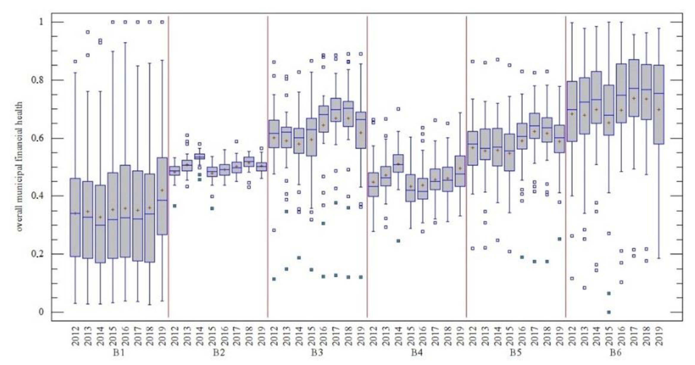
4.2. Assessment Based on Two Indicators (Variants B1, B2, B3, B4, B5, and B6)

This sub-section evaluates the financial health of municipalities using a pair of indicators, and the individual combinations are recorded in Figure 3. Within the terms of variants B1–B6, we use the results of the TOPSIS technique, which are standardised and fall within a range of <0;1> (see Figure 3).
In the case of assessment based on two indicators, we can easily observe differences in both distribution functions, the expected values, and the variability of the results. In assessing the overall financial health of the municipality, variant B1 identifies one subject from 2014 as the so-called PIS variant, i.e., the subject with the best results in both monitored indicators. These results are also stable over time (Q = 4.480; p = 0.7231) and balanced (LE = 0.118; p = 0.9975). The same is true for the results of variant B6. By using a pair of indicators within the terms of variant B2 (see Table 7), the expected values (Q = 70.852; p < 0.01) are statistically different while maintaining a similar dispersal range (LE = 0.7965; p = 0.5908). The same conclusions were observed for variants B3, B4, and B5.
When assessing the financial health of the municipalities via two indicators (Table 7), we repeatedly observed significant differences in overall standing based on the median throughout the entire monitored period. Significant deviations were also found in the differences between individual municipalities, as expressed by the variation range of the results from the TOPSIS technique. From this perspective, the municipalities are the most balanced when applying variant B2, while the greatest differences were observed under variant B1. However, the selection of a pair of indicators does not reflect the actual financial health of the assessed subject—in this case, the municipality. Based on these findings, we consider two criteria to be insufficient for complex assessment.

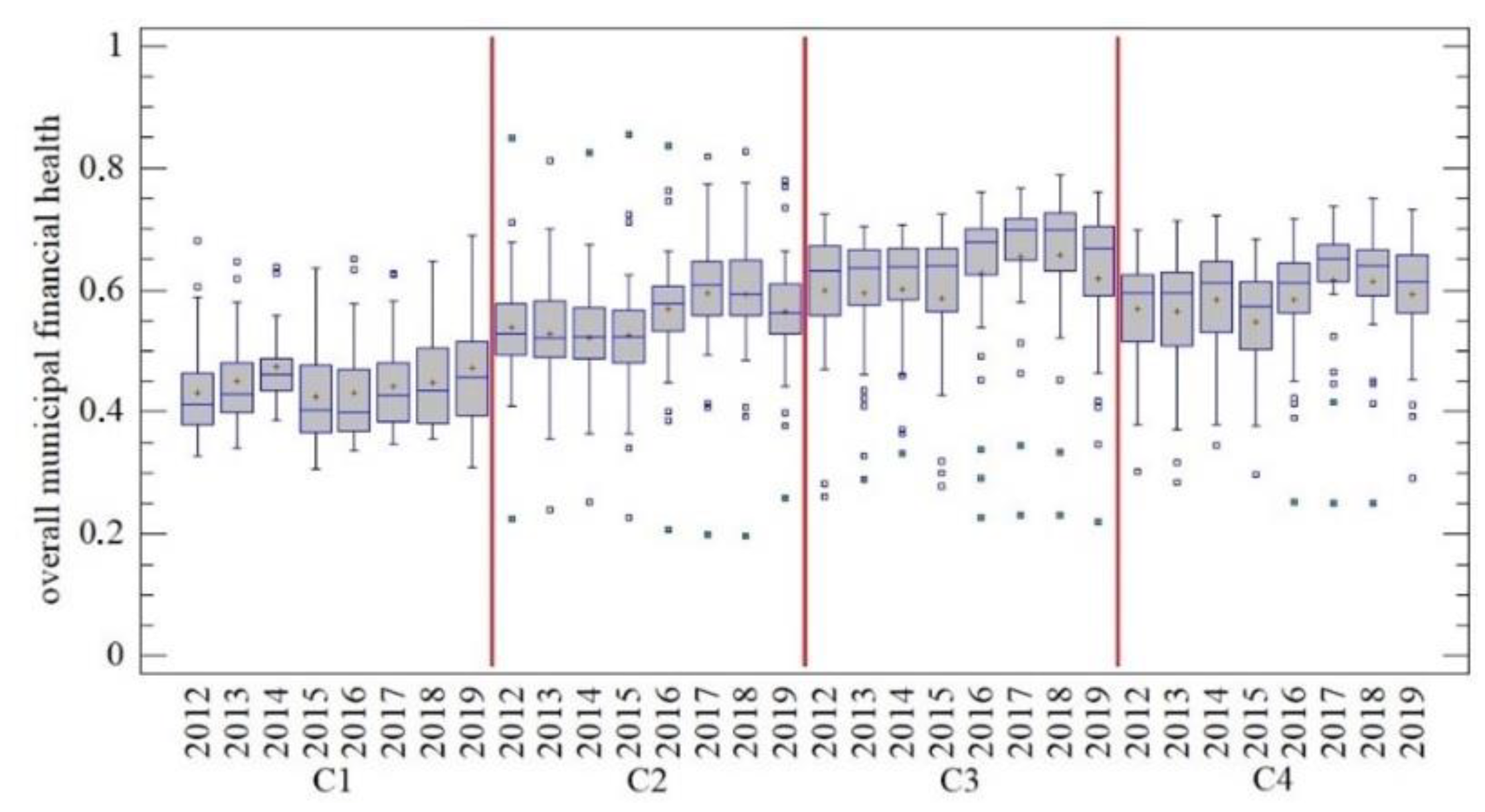
4.3. Assessment Based on Three Indicators (Variants C1, C2, C3, and C4)

In the case of the assessment of subjects within the terms of variants C1, C2, C3, and C4, we use a trio of indicators with a different nature (minimum versus maximum), which is also a significant factor affecting the assessment. In this case, the structure of the results is recorded in Figure 4.
In the case of assessment based on three indicators, we chiefly observed differences in the variation ranges and expected values of the acquired results (also shown in Figure 4). Within the terms of the results of variant C1, the differential year is 2014. Thus, we observed differences in the expected value (Q = 20.982; p = 0.0037) while maintaining the stable dispersion range of the results (LE = 1.318; p = 0.2420). The same is also true for the other three variants (C2, C3, C4), see Table 8.
The assessment of financial health based on three indicators better corresponds to the actual situation of the assessed subjects. This fact is also emphasised by the different natures of the assessed indicators, which were shown to conflict within the terms of the preceding assessment (see Section 4.1). This fact also contributed to the different order recorded in Table 8.

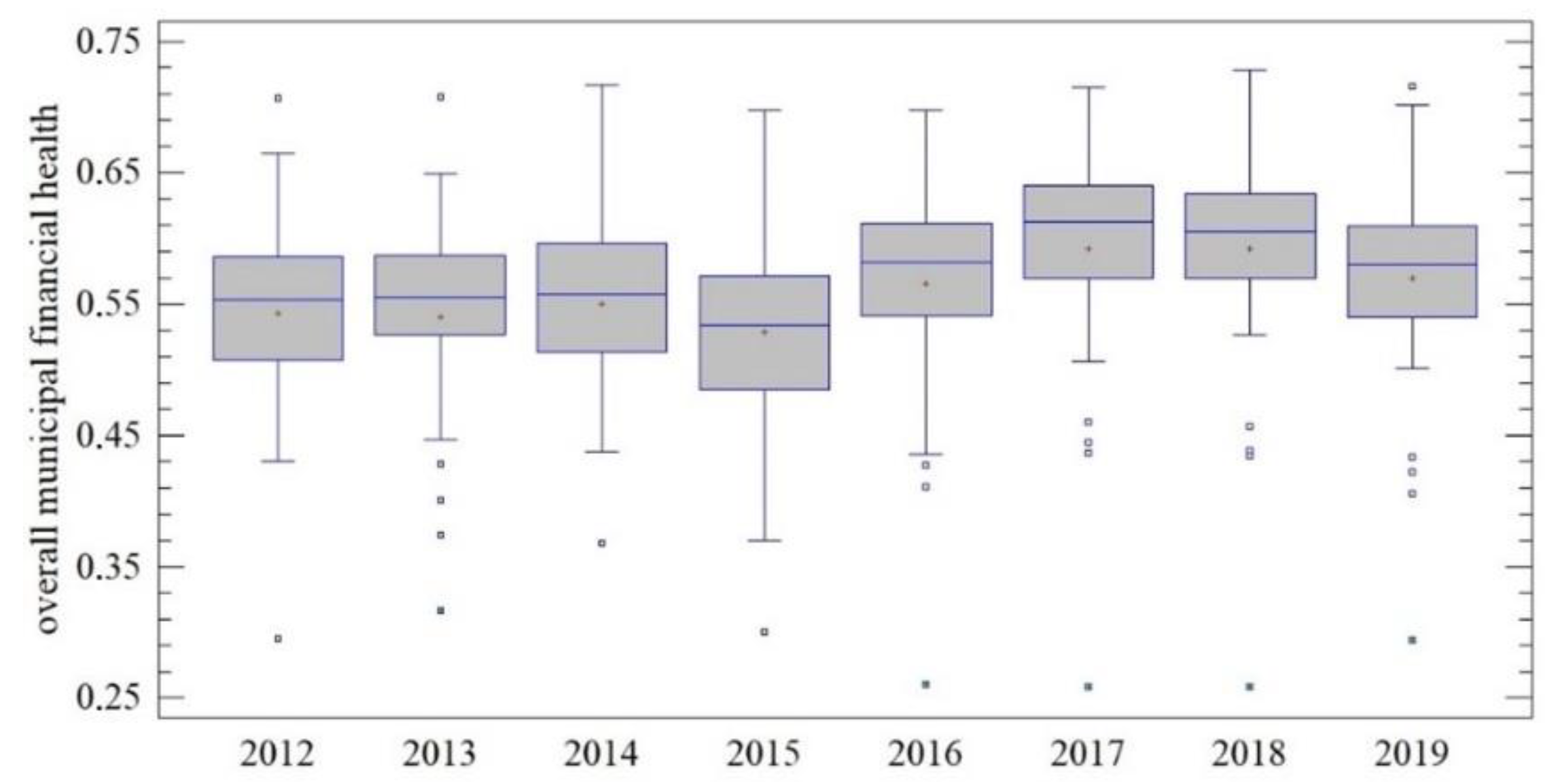
4.4. Assessment Based on Four Indicators (Variant D1)

Assessment of municipalities based on four indicators would reflect the actual situation of the assessed subjects better than the preceding cases. The results acquired in this manner are recorded in Figure 5. These results were affected by the occurrence of outlying observations (of subjects), which were observed during each assessment.
Despite the occurrence of outlying observations in the assessment based on four indicators, no differences were observed in the dispersion range of the results over the monitored period (LE = 0.061; p = 0.9997). The expected value of the results, which is also statistically significantly different (Q = 31.898; p ≤ 0.01), increased slightly over time.
The overall assessment recorded in Table 9 indicates relatively large differences between the assessed subjects (municipalities) with simultaneous minor year-on-year differences recorded using the decisive deviation or variation coefficient. Therefore, the differences persisted, and there is no presumption that these differences will be reduced or eliminated in the subsequent period.

4.5. Assessment of the Similarity of the Acquired Results

The key prerequisite for this paper was the selection of multiple indicators that best portray the actual situation of the individual subjects in the opinion of the assessor (or expert group). Therefore, we assumed that differences would arise from the number of assessed criteria, which was verified using the Jaccard index, as shown in Figure 6.
In each of the assessed years, we observed at least one variant, during which the Jaccard index is zero; i.e., the order of the subjects is completely different. From the perspective of assessment based on a single criterion, variant A4 gives the best assessment, i.e., assessment using the volume of liabilities per capita. However, in the context of the values of the Jaccard index, assessment using this indicator was still insufficient. For assessment using two indicators, the best results were achieved using a combination of the volume of total assets per capita (I2) and the volume of liabilities per capita (I4)—i.e., variant B5. The order obtained in this manner for 2019 copies at least 50% of the assessment using four monitored indicators. With three indicators, the best variant was C3 (all indicators with the exception of I3), but this this result did not exceed 31.25% order consistency.

5. Discussion and Conclusions

Multi-criteria assessment is an assessment and decision-making tool that is widely applied in different spheres of the private and public sectors, such as groundwater quality classification [47], tourism [48], energy policy [49], urban land use efficiency evaluation [50], transportation [51], and others. When applying each of these methods, an important step is to identify a set of relevant indicators and quantify their importance [52,53]. We identified four key indicators that can generally and complexly reflect the current situation of the assessed subjects; i.e., municipalities (and based on the specialist literature mentioned in Section 3.2). A homogenous group of 32 municipalities in the Czech Republic (see Section 3.1) was assessed. The intention was to demonstrate the importance of selecting suitable indicators for assessing the financial health of municipalities or the effectiveness of their management, which directly determined the results of the overall assessment. We can outline the following conclusions based on the results in this study:
  • The basis of assessment is the identification of a relevant set of alternatives (a criteria matrix), which should have similar attributes across the assessed subjects to the greatest degree possible; thus, the (partial) homogeneity of the assessed set is an essential prerequisite for assessment;
  • The selection of indicators that will subsequently be the subject of assessment should be subject to expert discussion or an extensive analysis of literary sources to demonstrate the justifiability of the specific criterion;
  • Assessment based on a low number of indicators is insufficient, highly variable, and diverse.
The results described above can be influenced to a specific degree by the selection of indicators and the research sample itself. Our goal was to objectivise the processes of indicator selection and processing as much as possible. Appropriate attention should be given to this step because incorrect determination directly and negatively impacts the results. Justification for using multi-criteria methods to complexly characterise the current situation was proven; these should be the primary methods used by decision-makers. Assessment based on a small number of subjective criteria can provide only partial information. This subsequently eliminates the application of such criteria within the terms of multi-criteria analysis to a specific degree. Therefore, we recommend using more indicators (at least four), thereby allowing evaluations to be more comprehensive and objective. Further research will focus on applications with a greater number of indicators to assess the differences. We also intend to apply different MCDM methods to generalise the results achieved.

Author Contributions

Conceptualisation, R.V.; methodology, R.V.; software, R.V.; validation, R.V.; formal analysis, R.V.; investigation, R.V., J.B., V.P. and P.G.; resources, R.V.; data curation, R.V., J.B., V.P. and J.M.; writing—original draft preparation, R.V.; writing—review and editing. R.V.; visualisation, R.V.; supervision, R.V.; project administration, R.V. and J.B.; funding acquisition, R.V and J.B. All authors have read and agreed to the published version of the manuscript.

Funding

This research was funded by the Student Grant Competition in VŠB—Technical University of Ostrava, grant number SP 2021/18” and by the Ministry of Education, Science, Research and Sport of the Slovak Republic, grant numbers VEGA 1/0578/18”, VEGA 1/0407/18”.

Data Availability Statement

Publicly available datasets were analysed in this study. These data can be found here: (Available online: https://monitor.statnipokladna.cz/ (accessed on 15 November 2020)).

Conflicts of Interest

The authors declare no conflict of interest.

References

  1. Hiadlovský, V.; Rybovičová, I.; Vinczeová, M. Importance of Liquidity Analysis in the Process of Financial Management of Companies Operating in the Tourism Sector in Slovakia: An Empirical Study. Int. J. Qua. Res. 2016, 10, 799–812. [Google Scholar]
  2. Jegers, M. Financing constraints in nonprofit organisations: A ‘Tirolean’ approach. J. Corp. Financ. 2011, 17, 640–648. [Google Scholar] [CrossRef]
  3. Grizzle, C.; Sloan, M.F.; Kim, M. Financial factors that influence the size of nonprofit operating reserves. J. Public Budg. Acc. Financ. Manag. 2015, 27, 67–97. [Google Scholar] [CrossRef]
  4. Michalski, G. Risk pressure and inventories levels. Influence of risk sensitivity on working capital levels. Econ. Comp. Econ. Cyb. Stud. Res. 2016, 50, 189–196. [Google Scholar]
  5. Gavurova, B.; Korony, S. Efficiency of day surgery in Slovak regions during the years 2009–2014. Econ. Ann. XXI 2016, 159, 80–84. [Google Scholar] [CrossRef] [Green Version]
  6. Šofránková, B.; Kiseľáková, D.; Horváthová, J. Actual questions of risk management in models affecting enterprise perfor-mance. Ekon. Čas. 2017, 65, 644–667. [Google Scholar]
  7. Lesáková, Ľ.; Vinczeová, M.; Ondrušová, A. Factors Determining Profitability of Small and Medium Enterprises in Selected Industry of Mechanical Engineering in the Slovak Republic—The Empirical Study. Ekon. Manag. 2019, 22, 144–160. [Google Scholar]
  8. Ochrana, F.; Pavel, J.; Vítek, L. Veřejný Sektor a Veřejné Finance. Financování Nepodnikatelských a Podnikatelských Aktivit; Grada Publishing: Prague, Czech Republic, 2010; pp. 1–30. [Google Scholar]
  9. Vavrek, R. Disparity of Evaluation of Municipalities on Region and District Level in Slovakia. In Proceedings of the Hradec Economic Day, Hradec Králové, Czechia, 3–4 February 2015. [Google Scholar]
  10. Otrusinova, M.; Kulleová, A. Liquidity Values in Municipal Accounting in Czech Republic. J. Comp. 2019, 11, 84–98. [Google Scholar] [CrossRef] [Green Version]
  11. Sebestova, J.; Majerova, I.; Szarowska, I. Indicators for assessing the financial condition and municipality management. Adm. Man. Pub. 2018, 31, 97–110. [Google Scholar]
  12. Sytnyk, N.; Onyusheva, I.; Holynskyy, Y. The managerial issues of state budgets execution: The case of Ukraine and Kazakhstan. Pol. J. Man. Stud. 2019, 19, 445–463. [Google Scholar] [CrossRef]
  13. Tkáčová, A.; Konečný, P. Krajské mestá Slovenska a ich finančné zdravie. Sci. Pap. Univ. Pard. Ser. D 2017, 41, 193–205. [Google Scholar]
  14. Adrian, T.; Covitz, D.; Liang, N. Financial stability monitoring. An. Rev. Fin. Econ. 2015, 7, 357–395. [Google Scholar] [CrossRef] [Green Version]
  15. Turco, M. The management of the financial collapse of local bodies and its economic-territorial effects: The case of the mu-nicipality of Taranto. Int. J. Pub. Sec. Perf. Man. 2017, 3, 191–207. [Google Scholar]
  16. Padovani, E.; Rossi, F.M.; Orelli, R.L. The Use of Financial Indicators to Determine Financial Health of Italian Municipalities. SSRN Electron. J. 2010. [Google Scholar] [CrossRef]
  17. Berne, R.; Schramm, R. The Financial Analysis of Governments; Prentice Hall: Englewood Cliffs, NJ, USA, 1986; pp. 1–30. [Google Scholar]
  18. McDonald, B.D. Measuring the Fiscal Health of Municipalities; Cambridge Press: Cambridge, UK, 2017; pp. 1–30. [Google Scholar]
  19. Tyson, C.J. Exploring the Boundaries of Municipal Bankruptcy. Will. Law Rev. 2014, 50, 661–683. [Google Scholar]
  20. Cabaleiro, R.; Buch, E.; Vaamonde, A. Developing a Method to Assessing the Municipal Financial Health. Am. Rev. Public Adm. 2012, 43, 729–751. [Google Scholar] [CrossRef]
  21. Halim, E.H.; Mustika, G.; Sari, R.N.; Anugerah, R.; Mohd-Sanusi, Z. Corporate governance practices and financial performance: The mediating effect of risk management committee at manufacturing firms. J. Int. Stud. 2017, 10, 272–289. [Google Scholar] [CrossRef] [PubMed] [Green Version]
  22. Zhatkin, Y.; Gurvits, N.; Strouhal, J. Addressing Ethical Matters in Ukrainian Accounting Practice. Econ. Sociol. 2017, 10, 167–178. [Google Scholar] [CrossRef] [PubMed] [Green Version]
  23. Opluštilová, I. Finanční Zdraví Obcí a Jeho Regionální Diferenciace; Masaryk University: Brno, Czech Republic, 2012; pp. 1–50. [Google Scholar]
  24. Peková, J.; Jetmar, M.; Tóth, P. Veřejný Sektor, Teorie a Praxe v ČR; Wolters Kluwer ČR: Prague, Czech Republic, 2019; pp. 325–337. [Google Scholar]
  25. Horvat, T.; Vidmar, M.; Justinek, G.; Bobek, V. Legislative, Organisational, and Economic Factors of Debt Level of Munici-palities in Slovenia. Lex Loc. J. Loc. Self-Gov. 2020, 18, 1067–1093. [Google Scholar]
  26. Brezovnik, B.; Finžgar, M.; Padovnik, S.A.; Mlinarič, F.; Oplotnik, Ž.J. Financing Municipal Tasks in Slovenia. Hrvat. Komparat. Javna Uprava 2019, 19, 173–206. [Google Scholar] [CrossRef]
  27. Dzialo, J.; Guziejewska, B.; Majdzinska, A.; Zoltaszek, A. Determinants of Local Government Deficit and Debt: Evidence from Polish Municipalities. Lex Loc. J. Loc. Self-Gov. 2019, 17, 1033–1056. [Google Scholar]
  28. Mihalovič, M. Performance Comparison of Multiple Discriminant Analysis and Logit Models in Bankruptcy Prediction. Econ. Sociol. 2016, 9, 101–118. [Google Scholar] [CrossRef] [PubMed]
  29. Mihalovič, M. Využitie skóringových modelov pri predikcii úpadku ekonomických subjektov v Slovenskej republike. Politická Ekon. 2018, 66, 689–708. [Google Scholar]
  30. Cohen, S.; Kaimenakis, N.; Venieris, G. Reaping the Benefits of Two Worlds: An Exploratory Study of the Cash and the Accrual Accounting Information Roles in Local Governments. J. App. Acc. Res. 2009, 14, 165–179. [Google Scholar] [CrossRef]
  31. Bellovary, J.L.; Giacomino, D.E.; Akers, M.D. A Review of Bankruptcy Prediction Studies: 1930-Present A Review of Bankruptcy Prediction Studies: 1930 to Present. J. Fin. Educ. 2007, 33, 1–43. [Google Scholar]
  32. Pereira, J.M.; Basto, M.; Da Silva, A.F. The Logistic Lasso and Ridge Regression in Predicting Corporate Failure. Procedia Econ. Financ. 2016, 39, 634–641. [Google Scholar] [CrossRef] [Green Version]
  33. Sun, J.; Li, H.; Huang, Q.H.; He, K.Y. Predicting financial distress and corporate failure: A review from the state-of-the-art definitions, modeling, sampling, and featuring approaches. Know. Bas. Sys. 2014, 57, 41–56. [Google Scholar] [CrossRef]
  34. Klepáč, V.; Hampel, D. Predicting financial distress of agriculture companies in EU. Agr. Econ. 2017, 63, 347–355. [Google Scholar]
  35. Papcunova, V. Evaluation of financial performance of contributory organizations under the jurisdiction of municipalities. Acta Reg. Environ. 2013, 10, 13–18. [Google Scholar] [CrossRef]
  36. Halásek, D.; Pilný, J.; Tománek, P. Určování Bonity Obcí; VŠB-TUO: Ostrava, Czech Republic, 2002; pp. 1–33. [Google Scholar]
  37. Provazníková, R. Financování Měst, Obcí a Regionů: Teorie a Praxe; Grada Publishing: Prague, Czech Republic, 2009; pp. 20–40. [Google Scholar]
  38. Malý, I.; Nemec, J. Možnosti Zvyšování Efektivnosti Veřejného Sektoru v Podmínkách Krize Veřejných Financí; Masaryk University: Brno, Czech Republic, 2011; pp. 1–40. [Google Scholar]
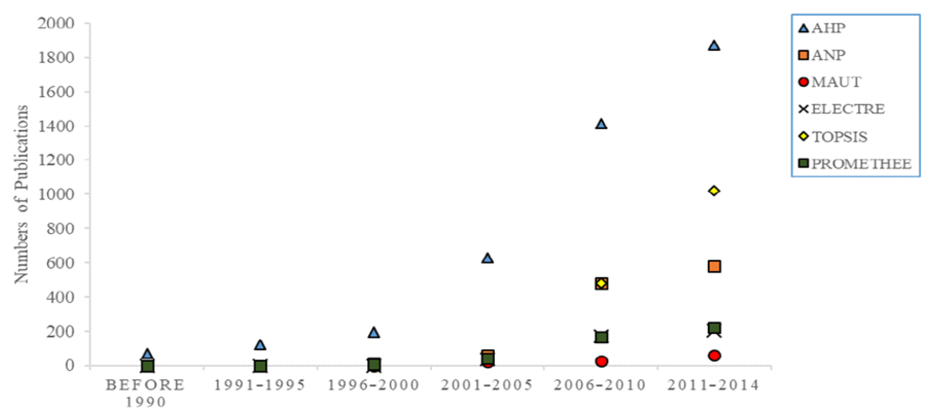
  39. Zavadskas, E.K.; Turskis, Z.; Kildienė, S. State of Art Surveys of Overviews on Mcdm/Madm Methods. Technol. Econ. Dev. Econ. 2014, 20, 165–179. [Google Scholar] [CrossRef] [Green Version]
  40. Hwang, C.L.; Yoon, K. Multiple Attributes Decision Making Methods and Applications; Springer: Berlin, Germany, 1981; pp. 1–15. [Google Scholar]
  41. Yoon, K. Systems Selection by Multiple Attribute Decision Making; Kansas State University: Manhattan, KS, USA, 1980; pp. 1–20. [Google Scholar]
  42. Tramarico, C.L.; Mizuno, V.; Antonio, V.; Salomon, P.; Augusto, F.; Marin, S. Analytic Hierarchy Process and Supply Chain Management: A Bibliometric Study. Proc. Comp. Scien. 2015, 55, 441–450. [Google Scholar] [CrossRef] [Green Version]
  43. Olson, D.L. Comparison of weights in TOPSIS models. Math. Comput. Model. 2004, 40, 721–727. [Google Scholar] [CrossRef]
  44. Streimikiene, D.; Balezentis, T.; Krisciukaitienė, I.; Balezentis, A. Prioritizing sustainable electricity production technologies: MCDM approach. Renew. Sustain. Energy Rev. 2012, 16, 3302–3311. [Google Scholar] [CrossRef]
  45. Zavadskas, E.K.; Mardani, A.; Turskis, Z.; Jusoh, A.; Nor, K. Development of TOPSIS Method to Solve Complicated Deci-sion-Making Problems: An Overview on Developments from 2000 to 2015. Int. J. Inf. Tech. Dec. Mak. 2016, 15, 1–38. [Google Scholar]
  46. Keršulienė, V.; Zavadskas, E.K.; Turskis, Z. SELECTION OF RATIONAL DISPUTE RESOLUTION METHOD BY APPLYING NEW STEP-WISE WEIGHT ASSESSMENT RATIO ANALYSIS (SWARA). J. Bus. Econ. Manag. 2010, 11, 243–258. [Google Scholar] [CrossRef]
  47. Zahedi, S.; Azarnivand, A.; Chitsaz, N. Groundwater quality classiffication derivation using multi-criteria-decision-making techniques. Ecol. Ind. 2017, 78, 243–252. [Google Scholar] [CrossRef]
  48. Yin, J.; Yang, X.Y.; Zheng, X.M.; Jiao, N.T. Analysis of the investment security of the accommodation industry for countries along the B&R: An empirical study based on panel data. Tour. Econ. 2017, 23, 1437–1450. [Google Scholar]
  49. Rozentale, L.; Blumberga, D. Methods to Evaluate Electricity Policy from Climate Perspective. Environ. Clim. Technol. 2019, 23, 131–147. [Google Scholar] [CrossRef] [Green Version]
  50. Zhang, L.; Zhang, L.; Xu, Y.; Zhou, P.; Yeh, C.-H. Evaluating urban land use efficiency with interacting criteria: An empirical study of cities in Jiangsu China. Land Use Policy 2020, 90, 104292. [Google Scholar] [CrossRef]
  51. Djodjević, B.; Krmac, E. Evaluation of energy-environment efficiency of European transport sectors: Non-radial DEA and TOPSIS approach. Energy 2019, 12, 2907. [Google Scholar]
  52. Brans, J.-P.; Mareschal, B. The PROMCALC & GAIA decision support system for multicriteria decision aid. Decis. Support Syst. 1994, 12, 297–310. [Google Scholar] [CrossRef]
  53. Yalcin, E.; Unlu, U. A multi-criteria performance analysis of initial public offering (IPO) firms using critic and vikor methods. Tech. Econ. Dev. Econ. 2018, 24, 534–560. [Google Scholar] [CrossRef]
Figure 1. Multi-criteria decision making methods used in 1990–2014.
Algorithms 14 00064 g001
Figure 2. The overall financial health of the municipality based on a single indicator (A1, A2, A3, A4) during the 2012–2019 period.
Algorithms 14 00064 g002
Figure 3. The overall financial health of municipalities based on two indicators (B1, B2, B3, B4, B5, and B6) during the 2012–2019 period.
Algorithms 14 00064 g003
Figure 4. The overall financial health of municipalities based on three indicators (C1, C2, C3, and C4) during the 2012–2019 period.
Algorithms 14 00064 g004
Figure 5. The overall financial health of municipalities based on four indicators (D1) during the 2012–2019 period.
Algorithms 14 00064 g005
Figure 6. Jaccard index of individual results with results from variant D1 by variant (a) and time (b).
Algorithms 14 00064 g006
Table 1. Coefficients and multiples of gradual transitions.
Municipalities with a Population Interval (from–to)Coefficient of Gradual TransitionsMultiple of Gradual Transitions
0–501.00001.0000 × the municipality’s population
51–20001.070050 + 1.0700 × number of residents of the municipality’s population exceeding 50
2001–30,0001.15232136.5 + 1.1523 × number of residents of the municipality’s population exceeding 2000
30,000 and more1.366334,400.9 + 1.3663 × number of residents of the municipality’s population exceeding 30,000
Table 2. List of names of municipalities included in the research sample.
Česká LípaJablonec nad NisouMostTábor
České BudějoviceJihlavaOlomoucTeplice
DěčínKarlovy VaryOpavaTrutnov
Frýdek-MístekKarvináPardubiceTřebíč
HavířovKladnoPísekTřinec
Hradec KrálovéKolínProstějovÚstí nad Labem
ChebLiberecPřerovZlín
ChomutovMladá BoleslavPříbramZnojmo
Table 3. Structure of indicators for the assessment of municipalities under the conditions of the Czech Republic (FAMA indicators).
Asset indicators: Value of assets per capita, Value of fixed tangible assets per capita, Value of land per capita, Value of structures per capita
Income indicators: Total income per capita, Own income per capita, Tax income per capita, Coefficient of the degree of self-sufficiency, Coefficient of the degree of dependence on non-recurring income, Regularly recurring income from assets, Regularly recurring income from fixed tangible assets, Regular income from structures
Expense indicators: Ordinary expenditures per capita, Capital expenses per capita, Total expenses per capita, Investment share coefficient
Combined indicators: Coefficient of the degree of coverage of ordinary expenditures, Gross savings, Coefficient of the degree of self-funding of investments, Coefficient of the degree of coverage of capital expenses, Coefficient of the degree of coverage of capital expenses from loans and obligations
Table 4. Structure of indicators within the terms of the system of informative and monitoring indicators (SIMU).
Informative indicators: Population of the municipality, Total income, Interest, Paid instalments on bonds and positive leverage, Debt service, Debt service indicator, Assets, Liabilities, Balance in bank accounts, Loan and communal bonds, Accepted repayable financial aid and other debts, Indebtedness, Share of indebtedness in liabilities, 8 year balance, Current assets, Short-term liabilities
Monitoring indicators: Ratio of liabilities to total assets, Total (current) liquidity
Table 5. Structure of the executed analysis depending on the number of assessed criteria.
Group DescriptionCombinations
A1 criterionA1(I1), A2(I2), A3(I3), A4(I4)
B2 criteriaB1(I1, I2), B2(I1, I3), B3(I1, I4), B4(I2, I3), B5(I2, I4), B6(I3, I4)
C3 criteriaC1(I1, I2, I3), C2(I1, I2, I4), C3(I1, I3, I4), C4(I2, I3, I4)
D4 criteriaD1(I1, I2, I3, I4)
Table 6. The best and the worst rated municipalities within the terms of variants A1, A2, A3, and A4 throughout the entire monitored period.
RankMED (A1)MED (A2)MED (A3)MED (A4)
1.M3028.069M30200.795M157.219M151.537
2.M2627.036M26181.783M218.350M281.792
3.M2726.764M32169.485M208.632M212.101
4.M2925.095M18134.463M229.567M142.401
5.M3224.892M29122.644M169.777M252.552
28.M2210.884M2051.318M2922.498M412.851
29.M1210.325M2148.230M3222.823M214.483
30.M208.858M1542.303M2723.111M2614.563
31.M218.722M2241.283M3025.579M3022.761
32.M158.468M1234.967M2626.131M124.930
Note: because the normality of the results was not confirmed, the median (MED) was chosen as the expected value.
Table 7. The best and the worst rated municipalities within the terms of variants B1, B2, B3, B4, B5, and B6 throughout the entire monitored period.
RankMED (B1)MED (B2)MED (B3)MED (B4)MED (B5)MED (B6)
1.M301.000M130.562M280.850M180.657M320.841M150.975
2.M260.871M100.519M290.838M300.594M280.747M210.953
3.M320.806M230.517M320.831M260.594M290.725M160.896
4.M290.610M220.516M250.704M100.573M180.715M140.896
5.M280.544M40.516M60.699M320.564M100.674M120.894
28.M200.080M70.491M80.550M120.398M270.456M20.480
29.M220.075M20.488M40.489M80.392M300.434M270.448
30.M210.072M320.487M20.394M40.363M20.415M260.406
31.M120.047M310.487M300.353M310.359M40.414M10.240
32.M150.037M60.475M10.125M270.299M10.214M300.157
Note: Since the normality of the results was not confirmed, the median (MED) was chosen as the expected value.
Table 8. The best- and the worst-rated municipalities within the terms of variants C1, C2, C3, and C4 throughout the entire monitored period.
RankMED (C1)MED (C2)MED (C3)MED (C4)
1.M300.642M320.826M280.743M180.716
2.M260.630M290.737M250.714M280.691
3.M320.610M280.734M140.710M320.683
4.M180.547M260.640M150.695M140.673
5.M100.533M180.639M210.690M100.667
28.M80.378M300.481M270.514M20.455
29.M150.374M80.465M260.503M40.446
30.M220.370M40.408M20.452M270.421
31.M40.358M20.396M300.333M300.407
32.M120.356M10.225M10.247M10.294
Note: Since the normality of the results was not confirmed, the median (MED) was chosen as the expected value.
Table 9. The best- and worst-rated municipalities within the terms of variant D1 throughout the entire monitored period.
RankMED (D1)
1.M320.695
2.M280.686
3.M180.653
4.M290.652
5.M100.635
28.M270.477
29.M300.452
30.M40.438
31.M20.435
32.M10.295
Note: Since the normality of the results was not confirmed, the median (MED) was chosen as the expected value.
Publisher’s Note: MDPI stays neutral with regard to jurisdictional claims in published maps and institutional affiliations.

