
Adaptive Behaviour for a Self-Organising Video Surveillance System Using a Genetic Algorithm


1
VTT—Technical Research Centre of Finland Ltd., MIKES bldg, Tekniikantie 1, 02150 Espoo, Finland
2
TNO—Netherlands Organisation for Applied Scientific Research, Oude Waalsdorperweg 63, 2597 AK Den Haag, The Netherlands
*
Author to whom correspondence should be addressed.
Algorithms 2021, 14(3), 74; https://0-doi-org.brum.beds.ac.uk/10.3390/a14030074
Submission received: 5 February 2021
/
Revised: 20 February 2021
/
Accepted: 22 February 2021
/
Published: 25 February 2021
(This article belongs to the Special Issue Nature Inspired Optimization Algorithms Recent Advances and Applications II)
Abstract
:Genetic algorithms (GA’s) are mostly used as an offline optimisation method to discover a suitable solution to a complex problem prior to implementation. In this paper, we present a different application in which a GA is used to progressively adapt the collective performance of an ad hoc collection of devices that are being integrated post-deployment. Adaptive behaviour in the context of this article refers to two dynamic aspects of the problem: (a) the availability of individual devices as well as the objective functions for the performance of the entire population. We illustrate this concept in a video surveillance scenario in which already installed cameras are being retrofitted with networking capabilities to form a coherent closed-circuit television (CCTV) system. We show that this can be conceived as a multi-objective optimisation problem which can be solved at run-time, with the added benefit that solutions can be refined or modified in response to changing priorities or even unpredictable events such as faults. We present results of a detailed simulation study, the implications of which are being discussed from both a theoretical and practical viewpoint (trade-off between saving computational resources and surveillance coverage).
1. Introduction
The Internet of Things (IoT) frequently involves retrofitting existing infrastructure with “intelligent” capabilities, see, e.g., in [1]. In turn, this requires identifying methods for turning an ad hoc collection of newly “connected” devices [2] into a cohesive whole capable of providing a better service than was previously achievable, due to the isolation of its various components [3]. This is often a challenging proposition and it could be argued that the IoT has so far failed to deliver on some ambitious promises of seamless interoperability and a step-change in how connected devices interact with their users and/or with each other. At least part of the reason is that the “augmentation” of pre-existing “things” with advanced communication and machine learning abilities is not enough. To recycle an iconic IoT meme: it is not because your fridge is now connected to the Internet that it will spontaneously enter a mutually beneficial relationship with the application responsible for monitoring the stock of fresh milk at your local supermarket. Even when possible in principle, useful interactions between “things” need to be identified and established carefully to provide any tangible benefits, which is far from trivial.
In this article, we are focusing using a genetic algorithm to engineer self-organisation into a population of devices which (a) were previously fulfilling a dedicated function (that might be impacted (positively or negatively) [1] by their new status as parts of a bigger whole) and which (b) could belong to different actors or organisations (that had never before cooperated and therefore may not have any agreement in place to realize this cooperation on an operational level, e.g., to share any resulting additional cost).
To illustrate this, we chose to investigate a specific—if hypothetical—scenario in which CCTV cameras in a shopping mall or retail space (street market, etc.) are being networked to provide an integrated video surveillance system [2]. The protection of public places through surveillance measures has been a concern for decades [4] and using the IoT to use existing infrastructure is a sustainable and cost-efficient approach.
Our hypothetical cameras belong to different shops where they were installed with the primary (and thus far only) objective to monitor the respective shops’ sensitive areas. There are solutions proposed in the literature to determine beneficial location, orientation and timing for integrated video surveillance systems (see, e.g., in [5]); however, in our case, the cameras’ locations and orientations are optimised subjectively by the shop owners without any organised pattern, resulting in partial overlap of coverage.
Using a genetic algorithm, we aim to optimise the system’s performance (i.e., the cost for—and the benefit generated from—operating it) by scheduling the individual camera’s activation. This is similar to solving a multi-objective optimisation problem:
- The cameras must spent as little time as possible in the “active” state [2] in which they are consuming resources such as power, network bandwidth, disk storage, screen space on the monitoring workstation, etc.
- The fraction of the shopping mall surface that is not being monitored (i.e., “blind spots”) should be minimised.
- The overlap between “active” cameras (i.e., zones that are being shown on several concurrent video feeds) is wasteful and must also be minimised.
We will show that once the alternative schedules are suitably encoded and a weighted fitness function has been specified, this multi-objective optimisation problem is easily and quickly solved by a genetic algorithm.
Genetic Algorithms (GAs) [6] are a nature-inspired [7] heuristic [8], i.e., an approach to find or estimate good solutions to a problem, as opposed to reliably determine the best one. Bio-inspired approaches apply principles found in nature [9] to improve algorithms [10]—often with very good results [11]. In the case of genetic algorithms [12], the principle of survival of the fittest is combined with the idea of mutation [13]: iteratively, the highest performing solutions from a set of candidate solutions are selected (performance-based selection) and subjected to local neighbourhood search (mutation) [14]. GAs have been used successfully in camera related optimisation problems, both for the placement of cameras [15] or for the interleaving of packets in messages sent by the cameras [16].
GAs—which are among the “most well-regarded evolutionary algorithms in history” [17] are mostly used as an offline optimisation method to discover a suitable solution to a complex problem prior to implementation. The idea to use them continuously at run-time is, of course, not new [18] (cf., e.g., in [19] for continuous portfolio optimisation, [20] for real-time task scheduling for multiprocessors or [21,22] for the optimisation of movement direction for the members of a drone swarm), but its by far not as popular as using them for a priori offline optimisation. In this paper, we apply the GA paradigm to the run-time adaption [23] of schedules for an ad hoc collection of cameras.
2. Schedule Encoding and Fitness Function
The genome we used is a two-dimensional binary array. Each line represents a camera and each column a time-slot in a periodic time window. A “1” indicates that the corresponding camera is in operation (i.e., streaming video) during a certain time-step while a “0” means that it is in stand-by mode.
Overlapping coverage is encoded as a three-dimensional binary matrix of size , with w and d the width and depth of the monitored area (in meters), and n the number of cameras. If the one cell centred on coordinates is within the field of view of a camera, then the corresponding entry is set to “1”. This information, while assumed to be known in our study a priori, could be generated relatively easily, be, e.g., moving a physical target over the area and recording which cameras are able to track it simultaneously (solutions to this are proposed in the literature, see, e.g., in [24]).
By cross-referencing this matrix with the activation schedule (genome), we determine whether a cell is being monitored by zero, one or more than one camera at any point in time. The area outside the field of view of any active cameras (“blind spots”) is measured by subtracting the surface being monitored (by all devices, taking any overlap into account, i.e., every m is only counted once) from the total area under surveillance.
The fitness function F only takes three global input variables: A (the total activation time for all cameras, equivalent to the number of 1’s in the schedule matrix; unit = s), B (the area of all “blind spots” over the duration of the periodic time-window; unit = ) and C (the overlapping coverage, i.e., the area being monitored by more than one camera over the duration of the periodic time-window; unit = ). Each variable’s impact on the overall fitness is weighted by tunable parameters , , and , respectively,
As all three input variables are to be minimised we are also interested in minimising F: the lower the value of F the fitter the schedule.
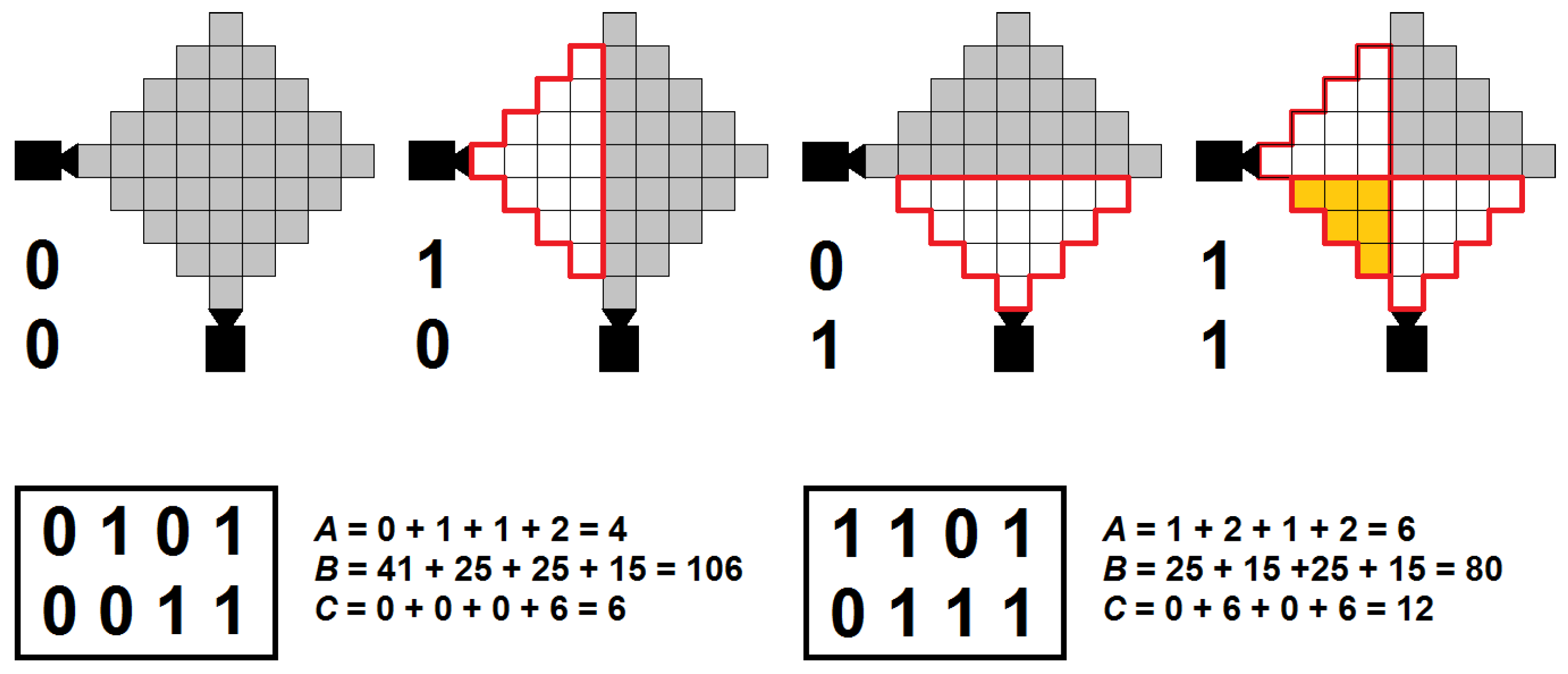
Our method is illustrated in Figure 1, for a simple 2-cameras example. The two boxes below the images represent two possible genomes, the images show the camera activation (over 4 times steps) defined in the genome on the left. In these genomes, the first line corresponds to the activation schedule of the first camera (horizontal orientation) and the second line to that of the second camera (vertical orientation). The red perimeter identifies the coverage area of each camera. Greyed squares are “blind spots” (not monitored), and orange squares are overlapping areas (monitored by more than one camera).
For example, to optimise coverage we might set the weighting parameter values to, e.g., , and . Under these settings, the schedule on the left in Figure 1 results in a fitness value F of 126 and is thus outperformed by the schedule on the right (score of 116). However, if we were more interested in saving resources, we might set to, e.g., 10 (while leaving the other parameters unchanged). Then, the schedule on the left scores 158 while the one on the right comes in at 164 (and thus the one on the left is better).
In order to make weighting more transparent and considering that the values for A, B, and C are dependent on experimental parameters such as the size of the area to be monitored, the number of cameras, the length of the periodic time window, etc., we defined secondary, dimensionless variables , , and as follows:
where stands for the maximum possible value of the corresponding variable. With respect to the example provided in Figure 1—with the maximum activation 8s (period (4s) × two cameras), the blind spots 41 × 4s = 164 and the overlap 6 × 4s = 24—the resulting values of , and are 0.5, ≈0.65, ≈0.33, and 0.75, ≈0.49 and ≈0.67 for the left and right schedule, respectively.
By choosing weighting parameters , , and such that
we ensure that the corresponding secondary fitness , defined as
is always comprised between 0 and 1. Unless stated otherwise, is the value reported for all numerical experiments in the remainder of this paper.
3. Genetic Algorithm, Reproduction, and Mutation/Selection Process
The GA was implemented as follows: on each generation, the fittest individuals (fixed fraction of the total population), each one carrying a genome representing one possible activation schedule, are selected to breed the next. Other individuals are eliminated and replaced by the offspring of the selected breeders. Unless stated otherwise, the best 25% of the individuals are allowed to survive and to pass on their genes. Each parent has three offspring, so as to keep the population constant.
In one version, reproduction is asexual (parthenogenesis) and the only genetic operator is mutation: every offspring in the new generation (75% of the population) starts as a clone of its single parent, then every bit in the two-dimensional genome “flips” with a uniform probability P (which, unless stated otherwise, is ).
In the second version, sexual (hermaphrodite) reproduction is implemented as follows: every surviving individual from the previous generation still “mothers” three offspring, but the genome of each one of them is the result of a combination of that of the “mother” with that of a “father”, randomly chosen among the other parents (each offspring can have a different “father”). Each column from the offspring’s genome/schedule (corresponding to every camera’s state during one given time-slot) is provided randomly (50% chance) by one of the parents. Mixing the parents’ genome lines was discarded because fitness heavily depends on the interoperation of cameras (e.g., overlap), effectively making substituting one schedule for another equivalent to random mutation.
Mutation operates in exactly the same way as for asexual reproduction (P = 0.01). The initial population is generated at random (every bit in the genome of every individual is randomly set to 0 or 1 with equal probability). Note that as parents (a) survive to the next generation, (b) are not subject to mutation and (c) are deterministically selected as the fittest, the best identified schedule is always retained.
4. Numerical Experiment Set-Up
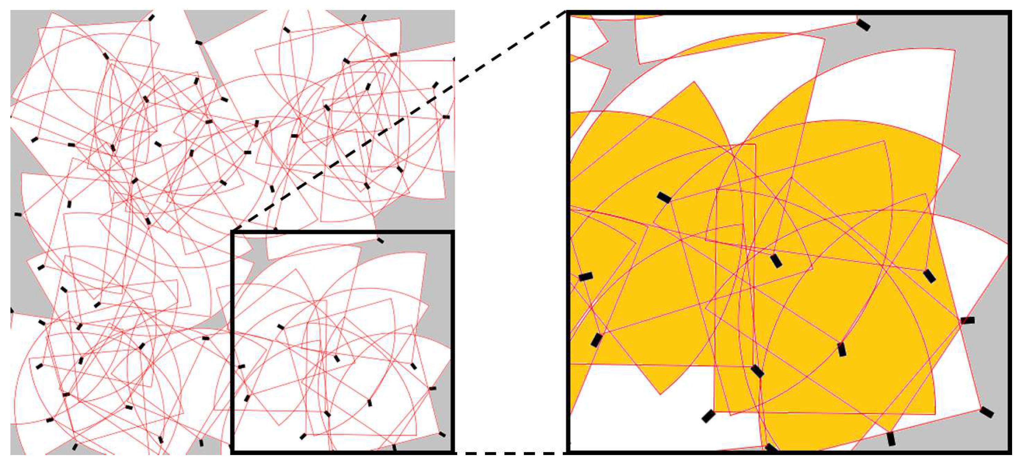
To test our method, we simulated m two-dimensional space monitored by 64 cameras. Each camera covers a “pie slice-shaped” area 90 degrees wide and 16 m deep (for an example, see Figure 2).
Cameras are randomly placed and oriented, within the limits of two constraints:
- No two cameras can be less than 4 m apart
- Cameras have at least 48 m from the monitored surface within their coverage area
The second constraint was introduced to ensure that cameras located on the edge of the set-up do not face outward. A typical example of the resulting environment is shown in Figure 2, using the same colour convention as in Figure 1.
The genetic pool is set to 64 individuals, with the 16 fittest (25%) surviving and breeding the next generation. The duration of the periodic time window is set to 32s (for comparison, the genome in Figure 1 covers only 4s), so the total size of the genome is 2048 bits (). The genetic algorithms is allowed to run for 10,000 generations, independently of reproduction type (parthenogenesis or hermaphrodite).
5. Limit-Cases and Benchmarking
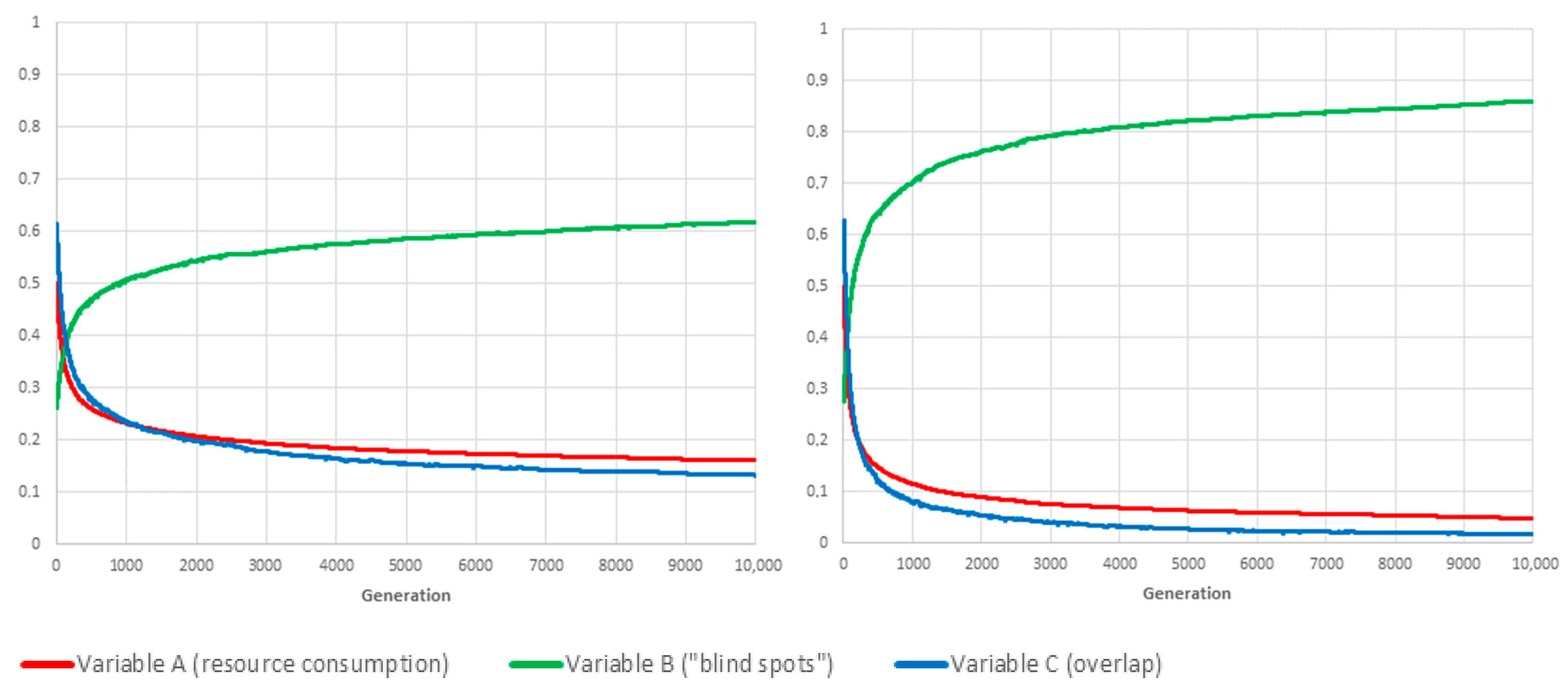
Limit-cases correspond to situations in which the value of one of the three weighting parameters , and is set to 1, which, according to the conservation law expressed by Equation (2), means that the other two global variables are not taken into account when computing fitness. As a benchmarking exercise, we investigated how our proposed genetic algorithm framework would deal with each of the three limit-cases, and for both reproduction methods. Figure 3, Figure 4 and Figure 5 show the resulting values for A, B and C when , and are evaluated in isolation, respectively.
If , the optimal solution is to permanently switch off all cameras ().
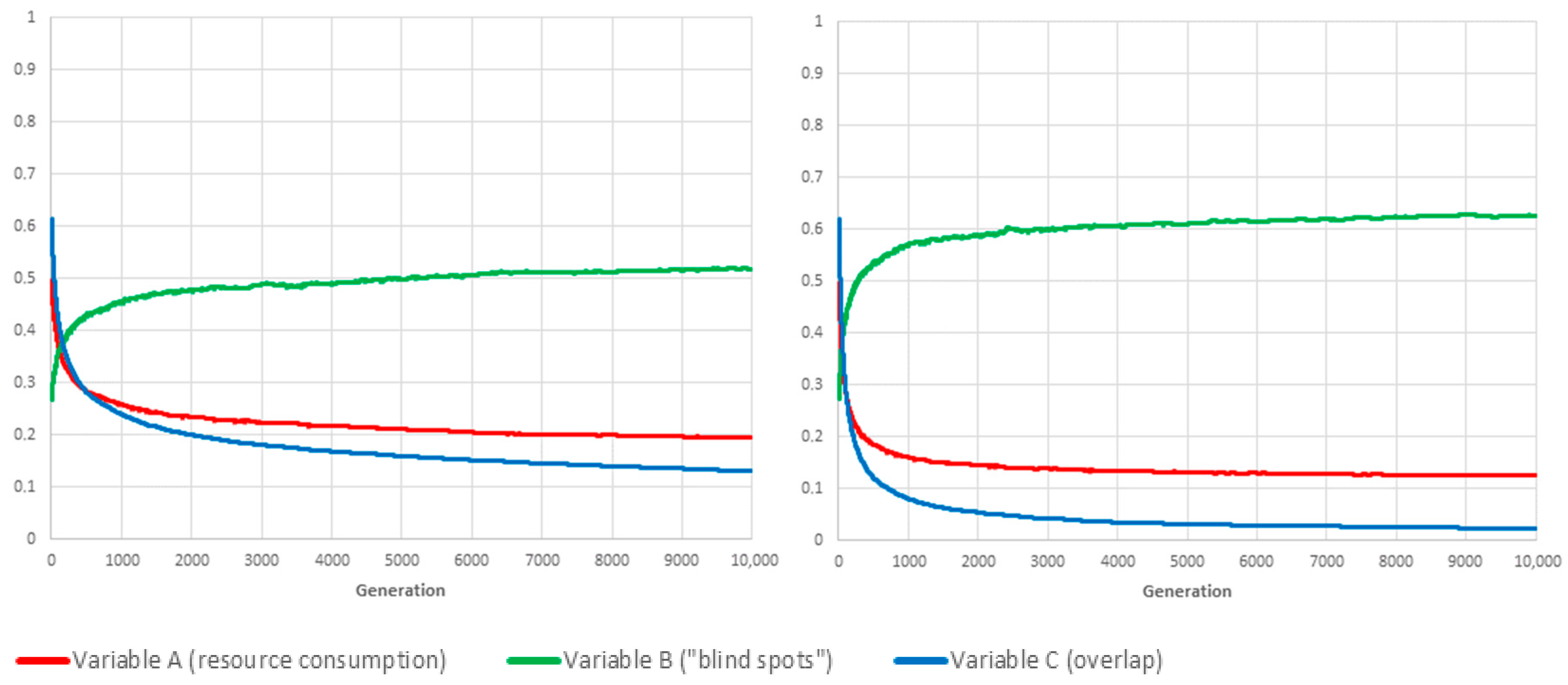
Symmetrically (see Figure 4), if , then one optimal solution is to never switch any of them off (although there will usually be others, in which some cameras, the coverage area of which is 100% overlapping with others, are permanently deactivated).
The third limit-case () has no such obvious optimum. Even though the optimal solution for is also one for , depending on cameras’ locations and orientations, there will usually be many other, less trivial schedules for which there is no overlapping coverage (C = 0).
The conclusion is twofold. First, the proposed framework is evidently capable of converging on the best schedule for each separate objective, namely, “lowest resource consumption” (), “fewest blind-spots” () and “minimal overlap” (). Second, the mixing of schedules/genes through sexual reproduction has, unsurprisingly, a very positive influence on the adaptation rate, especially when the objective is the conservation of resource or the avoidance of overlapping coverage.
6. Exploration of the Weighting Parameters Space
Because performance (rate of adaptation) is clearly better when using sexual reproduction (see Figure 5), all the following numerical experiments have been conducted using this method. The Monte Carlo simulation was implemented in Java. Each combination of weighting parameter values was the object of 180 independent realisations, each of them running for 10,000 generations. One realisation takes ≈4 min to complete on our Dell T7910 Workstation. Selected results are commented on below as well as presented as graphs in Figure 6, Figure 7 and Figure 8.
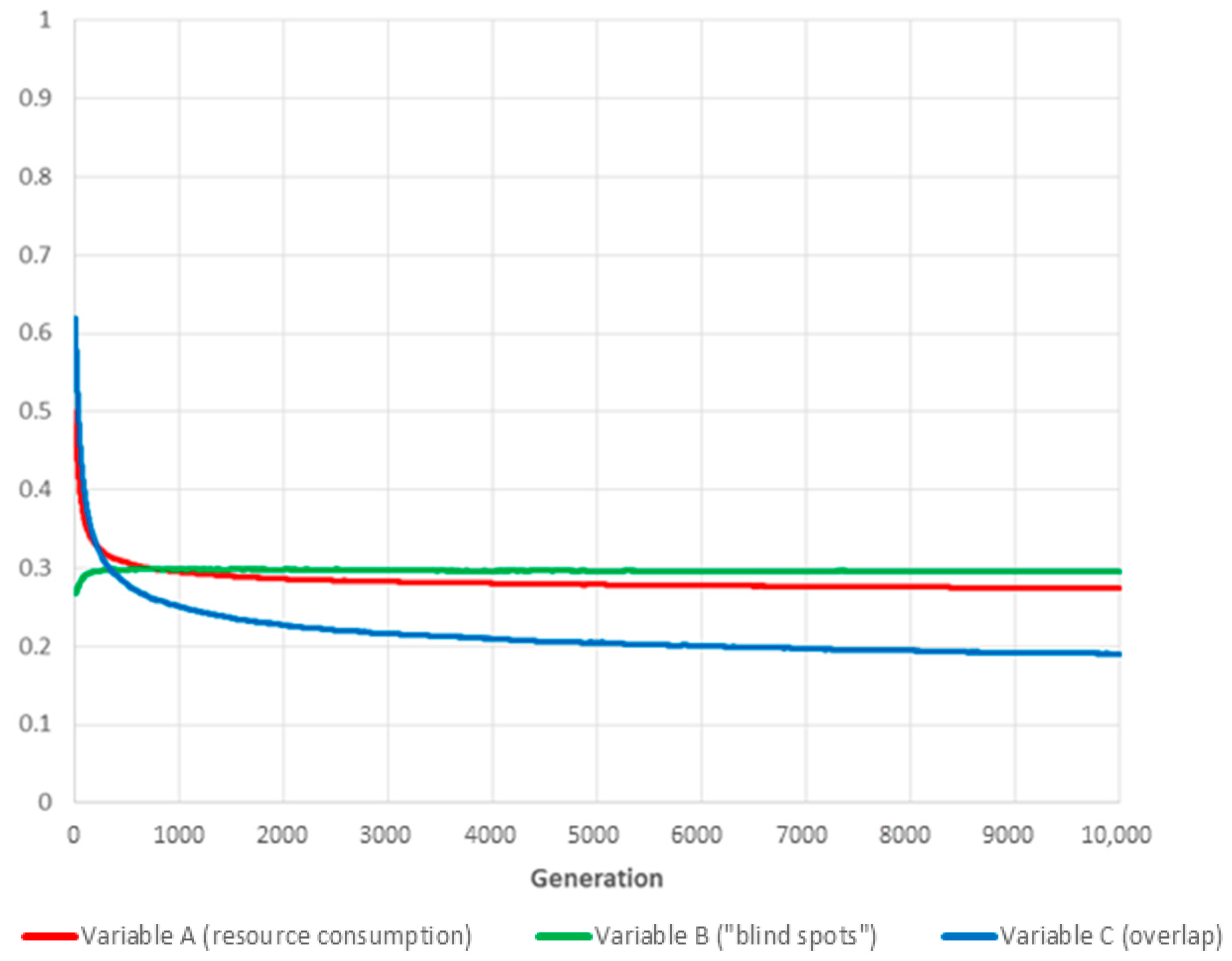
6.1. Case: (Equal Weights)
With equal weights, the most noticeable effect is that a combined reduction in resource consumption (variable A) and in overlap (variable C) is achieved at the expense of severely impaired coverage, which manifests itself as an increase in “blind spots” frequency (rising from about 25% in initial conditions to over 40%).
We attribute this result to the fact that the A and C variables are not fully independent in that they both benefit from switching off cameras indiscriminately. This would likely be unacceptable in a real-world deployment so the weight of the parameter should be increased to compensate for the combined effect of variables A and C.
6.2. Case: ,
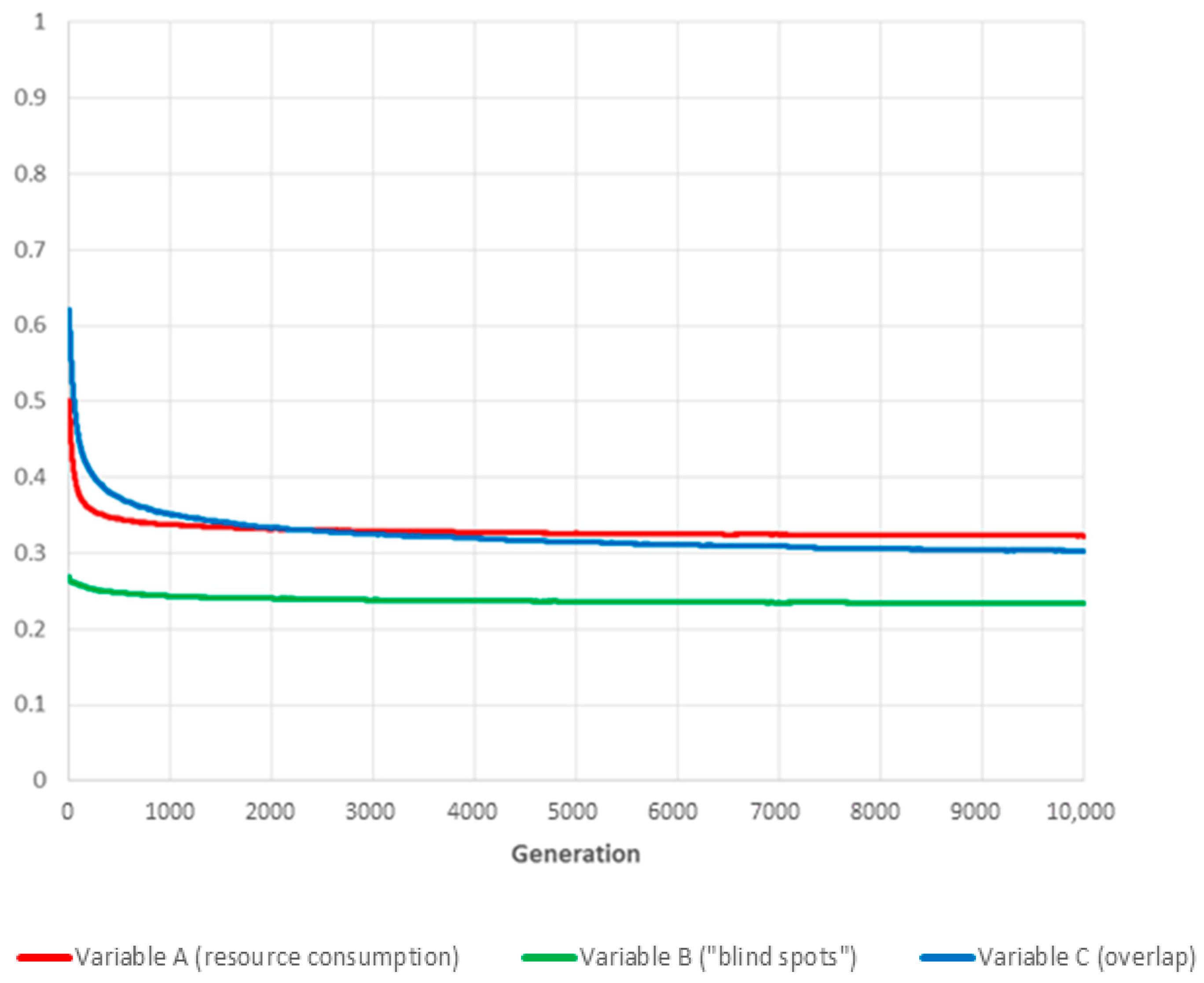
Increasing the weight of variable B (“blind spots”) unsurprisingly improves coverage while simultaneously reducing benefits in terms of minimising resource usage and overlap. However, “blind spots” still increase compared to random initial conditions, albeit only by a marginal fraction.
6.3. Case: ,
More surprisingly, in our exploration of the weighting parameters space, completely eliminating overlap from the fitness evaluation by assigning a value of zero to parameter gave the best result, with strong to moderate improvements across all three performance measurement variables.
Our interpretation is that this is caused by the high density of cameras in the numerical experiment set-up, which leads to substantial overlap (see Figure 2). Consequently, explicitly trying to minimise the corresponding variable C forces the evolutionary process to switch off cameras more often than is desirable from a coverage point of view, creating “blind spots” in areas monitored by just one camera in an attempt to minimise partial overlap with other nearby devices.
7. Run-Time Adaptation and Real-World Considerations
One salient feature of our genetic algorithm framework is that it is not designed for offline multi-objective optimisation, but intended as a run-time method to improve the performance of an integrated video surveillance system “on-the-fly”. This includes the ability to respond to disruptive events, such as the failure of cameras, by adaptively reorganising the schedule of other devices so as to compensate for the loss of coverage consecutive to the fault.
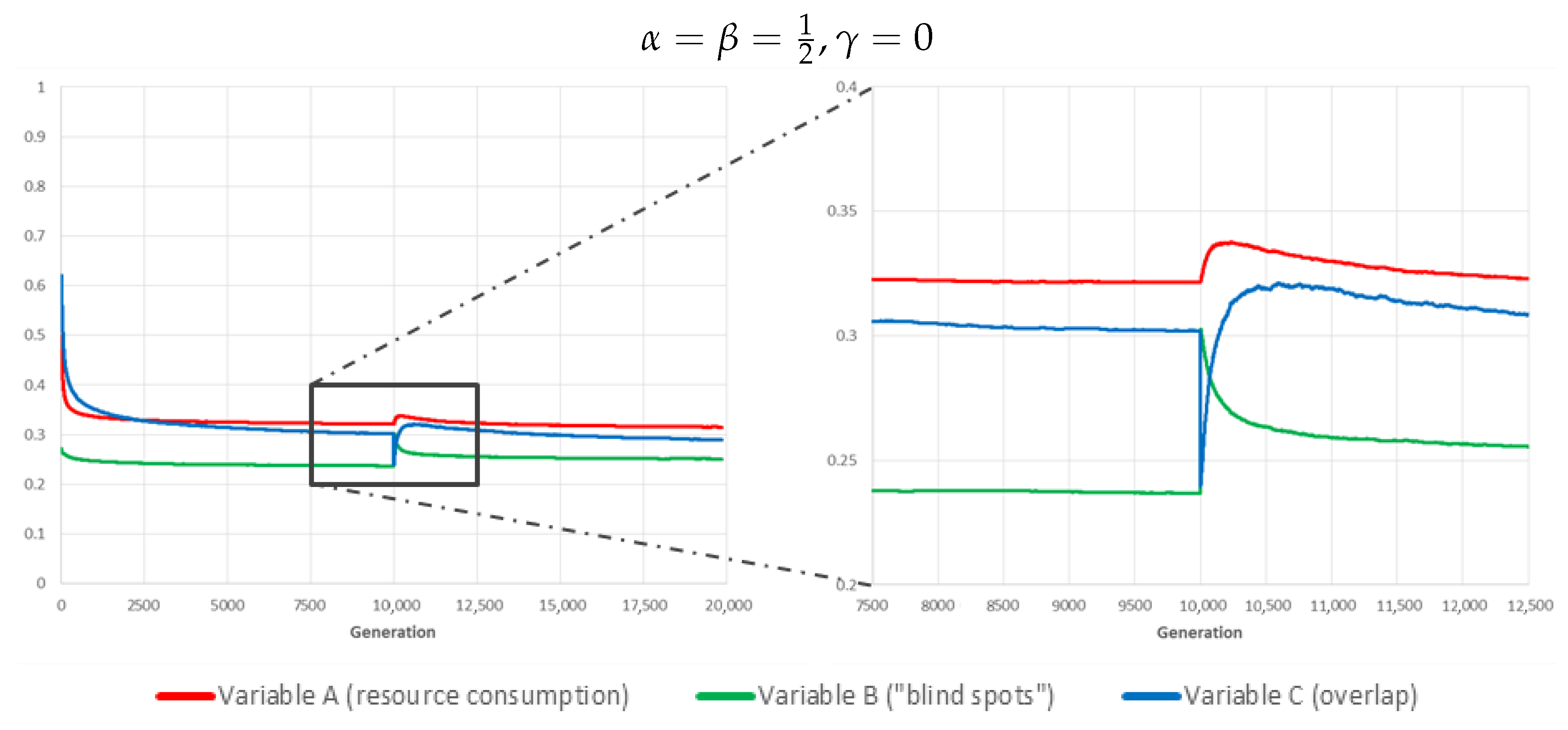
To demonstrate this ability, we ran a separate batch of simulations, using the best identified weighting parameter values (, ), in which 8 randomly chosen cameras (out of 64) are “deactivated” at generation 10,000, and the system is allowed to recover for another 10,000 generations after the event (during which the impacted devices remain permanently offline), see Figure 9.
As expected, the sudden failure results in a sharp rise in the value of variable B (“blind spots”). This boosts the relative fitness of genomes/schedules in which other cameras are activated more often, leading to a temporary rise in variables A and C, following a sharp drop of the latter consecutive to the disappearance of overlap with faulty devices (note that these are still consuming resources in our scenario, so variable A is unaffected). After a few hundred to a thousand generations though, the system has successfully adapted and all variables have resumed a downward trend, albeit the fact that variable B is necessarily converging to a higher plateau (this is necessarily so because some of the new “blind spots” are out of coverage for all surviving cameras).
We argue that our method, although clearly perfectible, is already suitable for real-world deployment “as is” and offers immediate benefits. It is straightforward and not particularly computationally intensive to evaluate one generation per second (in our simulations, we do over 40 over the same period), so for a system of the size envisaged (64 cameras, 32 s periodic time window), identifying a suitable schedule would take a few minutes to a few hours. More importantly, the system would respond to a disruptive event over a similar time-scale, making run-time adaptation very feasible.
In terms of resource-saving performance, the benefit is roughly a rd reduction compared to an “always-on” schedule. This obviously means that for the same disk storage capacity, archived footage would cover a period three times longer, e.g., 72 h instead of a single day. By way of contrast, the loss of coverage resulting from this adaptation only represents about 10% of the monitored area (note that this does not mean that these additional 10% are never monitored, only that they are filmed less often). Although we fully acknowledge that these results are sensitive to the value of the parameters used for the numerical experiment (number of cameras, field of view, etc.), there is no reason to believe that they would be qualitatively different in other scenarios.
8. Conclusions and Future Work
We have presented what we believe to be a fully specified framework for orchestrating the operation of an ad hoc video surveillance system using a genetic algorithm to achieve multi-objective optimisation at run-time, in a dynamic environment. Simulation results demonstrate that the proposed approach can save valuable resources (network bandwidth, storage space, etc.) without significantly compromising coverage, as well as responding quickly and efficiently to disruptive events.
We fully acknowledge that additional effort is required before such a system can be deployed in the real world. This future work can roughly be divided into two categories:
- There is room for further practical development on the implementation side, specifically with regard to the design of reliable techniques to acquire the information “consumed” by the genetic algorithm’s fitness function. For example, even though we do not think that this represents in any way an unsurmountable obstacle, measuring overlap between cameras could be a challenge in its own right. It is not hard to imagine empirical methods, such as target tracking in a pre-deployment training phase, to obtain a rough approximation (e.g., a binary matrix showing which pairs of cameras do and do not overlap), but making a more precise estimate (e.g., the surface of the overlapping coverage area) could prove difficult. However, as automated surveillance is a rapidly growing market, solutions to this challenge are being worked on. Furthermore, our numerical experiments indicate that this is the least critical of the three fitness variables, so it is certainly no “show stopper”.
- More exploration of the parameters space is required to quantify the influence of external parameters over the performance of the adaptive framework, and to determine the best internal parameter values for any given deployment scenario. The difficulty here comes from the large number of external parameters, some of which might not even have been identified yet, which, together with the very wide range of possible values for them, make a systematic approach unrealistic. We will focus our own efforts on scale (i.e., number and density of cameras) as we suspect they might have the strongest impact on the possible benefits of incorporating overlap into the fitness function. There are, however, many other aspects to document. In particular, it would be desirable to improve the way in which coverage is modelled, for instance, by taking into account distance from the camera and substituting a continuous variable (image quality) to our binary one.
By describing our method and publishing our results at this intermediate stage, we hope to encourage the community to extend and complement this work. We believe that it represents a promising and credible run-time application of genetic algorithms, of which there are relatively few examples.
Author Contributions
Conceptualization, F.S.; Data curation, F.S.; Formal analysis, F.S. and H.H.; Funding acquisition, F.S.; Investigation, F.S. and H.H.; Methodology, F.S.; Project administration, F.S.; Resources, F.S.; Software, F.S.; Validation, F.S. and H.H.; Visualization, F.S.; Writing—original draft, F.S. and H.H.; Writing—review & editing, F.S. and H.H. All authors have read and agreed to the published version of the manuscript.
Funding
This research received no external funding.
Conflicts of Interest
The authors declare no conflict of interest.
References
- Medina, B.E.; Manera, L.T. Retrofit of air conditioning systems through an Wireless Sensor and Actuator Network: An IoT-based application for smart buildings. In Proceedings of the 2017 IEEE 14th International Conference on Networking, Sensing and Control (ICNSC), Calabria, Italy, 16–18 May 2017; pp. 49–53. [Google Scholar] [CrossRef]
- Cao, N.; Nasir, S.B.; Sen, S.; Raychowdhury, A. Self-Optimizing IoT Wireless Video Sensor Node With In-Situ Data Analytics and Context-Driven Energy-Aware Real-Time Adaptation. IEEE Trans. Circuits Syst. I Regul. Pap. 2017, 64, 2470–2480. [Google Scholar] [CrossRef]
- Vespignani, A. The fragility of interdependency. Nature 2010, 464, 984–985. [Google Scholar] [CrossRef] [PubMed]
- Svenonius, O. The body politics of the urban age: Reflections on surveillance and affect. Palgrave Commun. 2018, 4, 2. [Google Scholar] [CrossRef] [Green Version]
- Jun, S.; Chang, T.W.; Jeong, H.; Lee, S. Camera Placement in Smart Cities for Maximizing Weighted Coverage with Budget Limit. IEEE Sensors J. 2017, 17, 7694–7703. [Google Scholar] [CrossRef]
- Goodman, E.D. Introduction to Genetic Algorithms. In Proceedings of the 14th Annual Conference Companion on Genetic and Evolutionary Computation; ACM: New York, NY, USA, 2012; pp. 671–692. [Google Scholar] [CrossRef]
- Sarmah, D.K. A Survey on the Latest Development of Machine Learning in Genetic Algorithm and Particle Swarm Optimization. In Optimization in Machine Learning and Applications; Kulkarni, A.J., Satapathy, S.C., Eds.; Springer: Singapore, 2020; pp. 91–112. [Google Scholar] [CrossRef]
- Pearl, J. Heuristics: Intelligent Search Strategies for Computer Problem Solving; The Addison-Wesley Series in Artificial Intelligence; Addison-Wesley: Boston, MA, USA, 1984. [Google Scholar]
- Bonabeau, E.; Dorigo, M.; Theraulaz, G. Inspiration for optimization from social insect behaviour. Nature 2000, 406, 39–42. [Google Scholar] [CrossRef] [PubMed]
- Navlakha, S.; Bar-Joseph, Z. Algorithms in nature: The convergence of systems biology and computational thinking. Mol. Syst. Biol. 2011, 7. [Google Scholar] [CrossRef] [PubMed]
- Bartholdi, J.J.; Eisenstein, D.D. A Production Line that Balances Itself. Oper. Res. 1996, 44, 21–34. [Google Scholar] [CrossRef]
- Rowe, J.E. Genetic Algorithm Theory. In Proceedings of the 9th Annual Conference Companion on Genetic and Evolutionary Computation; ACM: New York, NY, USA, 2007; pp. 3585–3608. [Google Scholar] [CrossRef]
- Padhye, N. Evolutionary Approaches for Real World Applications in 21st Century. In Proceedings of the 14th Annual Conference Companion on Genetic and Evolutionary Computation; ACM: New York, NY, USA, 2012; pp. 43–48. [Google Scholar] [CrossRef]
- Mitchell, M. An Introduction to Genetic Algorithms; A Bradford book; The MIT Press: Cambridge, MA, USA, 1998. [Google Scholar]
- Jun, S.; Chang, T.W.; Yoon, H.J. Placing Visual Sensors Using Heuristic Algorithms for Bridge Surveillance. Appl. Sci. 2018, 8, 70. [Google Scholar] [CrossRef] [Green Version]
- Zapata-Quiñones, K.; Duran-Faundez, C.; Gutiérrez, G.; Lecuire, V.; Arredondo-Flores, C.; Jara-Lipán, H. A Genetic Algorithm for the Generation of Packetization Masks for Robust Image Communication. Sensors 2017, 17, 981. [Google Scholar] [CrossRef] [PubMed] [Green Version]
- Mirjalili, S.; Song Dong, J.; Sadiq, A.S.; Faris, H. Literature Review, and Application in Image Reconstruction. In Nature-Inspired Optimizers: Theories, Literature Reviews and Applications; Mirjalili, S., Song Dong, J., Lewis, A., Eds.; Springer International Publishing: Cham, Switzerland, 2020; pp. 69–85. [Google Scholar] [CrossRef]
- Akimoto, Y.; Auger, A.; Hansen, N. Introduction to Randomized Continuous Optimization. In Proceedings of the 2016 on Genetic and Evolutionary Computation Conference Companion; GECCO ’16 Companion; ACM: New York, NY, USA, 2016; pp. 333–355. [Google Scholar] [CrossRef]
- Kessaci, Y. A Multi-objective Continuous Genetic Algorithm for Financial Portfolio Optimization Problem. In Proceedings of the Genetic and Evolutionary Computation Conference Companion; GECCO ’17; ACM: New York, NY, USA, 2017; pp. 151–152. [Google Scholar] [CrossRef]
- Gharsellaoui, H.; Ktata, I.; Kharroubi, N.; Khalgui, M. Real-time reconfigurable scheduling of multiprocessor embedded systems using hybrid genetic based approach. In Proceedings of the 2015 IEEE/ACIS 14th International Conference on Computer and Information Science (ICIS), Las Vegas, NV, USA, 28 June–1 July 2015; pp. 605–609. [Google Scholar] [CrossRef]
- Hildmann, H.; Eledlebi, K.; Saffre, F.; Isakovic, A.F. Chapter: The swarm is more than the sum of its drones—A swarming behaviour analysis for the deployment of drone-based wireless access networks in GPS-denied environments and under model communication noise. In Internet of Drones; Studies in Systems, Decision and Control; Springer: Berlin/Heidelberg, Germany, 2021. [Google Scholar]
- Eledlebi, K.; Ruta, D.; Hildmann, H.; Saffre, F.; Alhammadi, Y.; Isakovic, A.F. Coverage and Energy Analysis of Mobile Sensor Nodes in Obstructed Noisy Indoor Environment: A Voronoi-Approach. IEEE Trans. Mob. Comput. 2020, 1. [Google Scholar] [CrossRef]
- Pascual, G.G.; Pinto, M.; Fuentes, L. Run-time adaptation of mobile applications using genetic algorithms. In Proceedings of the 2013 8th International Symposium on Software Engineering for Adaptive and Self-Managing Systems (SEAMS), San Francisco, CA, USA, 20–21 May 2013; pp. 73–82. [Google Scholar] [CrossRef] [Green Version]
- Teklehaymanot, F.K.; Muma, M.; Zoubir, A.M. Adaptive diffusion-based track assisted multi-object labeling in distributed camera networks. In Proceedings of the 2017 25th European Signal Processing Conference (EUSIPCO), Kos, Greece, 28 August–2 September 2017; pp. 2299–2303. [Google Scholar] [CrossRef] [Green Version]
Figure 1.
Schedule encoding scheme and evaluation of the input variables to the fitness function, for a two-cameras example (two rows) and a four steps periodic time-window (four columns).
Figure 1.
Schedule encoding scheme and evaluation of the input variables to the fitness function, for a two-cameras example (two rows) and a four steps periodic time-window (four columns).

Figure 2.
A typical environment semi-randomly generated for the numerical experiment setup. Colour as in Figure 1: the zoomed-in picture on the right shows overlap (orange area) if all cameras are turned on. Note the “blind spots” (grey area) that are permanently outside coverage.
Figure 2.
A typical environment semi-randomly generated for the numerical experiment setup. Colour as in Figure 1: the zoomed-in picture on the right shows overlap (orange area) if all cameras are turned on. Note the “blind spots” (grey area) that are permanently outside coverage.

Figure 3.
Benchmarking tests: We show the evolution over time of variables A, B and C for the fittest individual of each generation (the plotted values are averaged over 20 independent realisations). If then ; and F is equal to A. Consequently, the GA is optimising F by reducing the value of A to (eventually) zero. The convergence speed of the algorithm when using mutation only (left panel) is significantly slower than with sexual reproduction (right panel).

Figure 4.
Benchmarking tests: i.e., the value of F is only based on blind spots. Both variations (left: mutation only; right: with sexual reproduction) perform comparable, the value of B may never drop entirely to zero due to unavoidable blind spots caused by the camera placement.
Figure 4.
Benchmarking tests: i.e., the value of F is only based on blind spots. Both variations (left: mutation only; right: with sexual reproduction) perform comparable, the value of B may never drop entirely to zero due to unavoidable blind spots caused by the camera placement.

Figure 5.
Benchmarking tests: setting implies (as above) that only one value contributes to F, namely, C, the overlap. In both variations of the GA C is being reduced but the GA with sexual reproduction (right panel) significantly outperforms the variation that uses only mutation (left).
Figure 5.
Benchmarking tests: setting implies (as above) that only one value contributes to F, namely, C, the overlap. In both variations of the GA C is being reduced but the GA with sexual reproduction (right panel) significantly outperforms the variation that uses only mutation (left).

Figure 6.
The curves show the evolution over time of the three global variables (for the values ) for the fittest individual of each generation (reported are the averaged values over 180 independent realisations).
Figure 6.
The curves show the evolution over time of the three global variables (for the values ) for the fittest individual of each generation (reported are the averaged values over 180 independent realisations).

Figure 7.
The curves show the evolution over time of the three global variables (for the values ) for the fittest individual of each generation (the shown results are averaged over 180 independent realisations).
Figure 7.
The curves show the evolution over time of the three global variables (for the values ) for the fittest individual of each generation (the shown results are averaged over 180 independent realisations).

Figure 8.
The curves show the evolution over time of the three global variables (for the values ) for the fittest individual of each generation (the presented results are the averages over 180 independent realisations).
Figure 8.
The curves show the evolution over time of the three global variables (for the values ) for the fittest individual of each generation (the presented results are the averages over 180 independent realisations).

Figure 9.
Response to a disruptive event (failure of 8 out of 64 cameras at generation 10,000). The curves show the evolution over time of the three global variables for the fittest individual of each generation (averaged over 180 independent realisations).
Figure 9.
Response to a disruptive event (failure of 8 out of 64 cameras at generation 10,000). The curves show the evolution over time of the three global variables for the fittest individual of each generation (averaged over 180 independent realisations).

Publisher’s Note: MDPI stays neutral with regard to jurisdictional claims in published maps and institutional affiliations. |
© 2021 by the authors. Licensee MDPI, Basel, Switzerland. This article is an open access article distributed under the terms and conditions of the Creative Commons Attribution (CC BY) license (http://creativecommons.org/licenses/by/4.0/).
Share and Cite
MDPI and ACS Style
Saffre, F.; Hildmann, H. Adaptive Behaviour for a Self-Organising Video Surveillance System Using a Genetic Algorithm. Algorithms 2021, 14, 74. https://0-doi-org.brum.beds.ac.uk/10.3390/a14030074
AMA Style
Saffre F, Hildmann H. Adaptive Behaviour for a Self-Organising Video Surveillance System Using a Genetic Algorithm. Algorithms. 2021; 14(3):74. https://0-doi-org.brum.beds.ac.uk/10.3390/a14030074
Chicago/Turabian StyleSaffre, Fabrice, and Hanno Hildmann. 2021. "Adaptive Behaviour for a Self-Organising Video Surveillance System Using a Genetic Algorithm" Algorithms 14, no. 3: 74. https://0-doi-org.brum.beds.ac.uk/10.3390/a14030074
Note that from the first issue of 2016, this journal uses article numbers instead of page numbers. See further details here.