
Feature and Language Selection in Temporal Symbolic Regression for Interpretable Air Quality Modelling


1
Department of Mathematics and Computer Science, University of Ferrara, 44121 Ferrara, Italy
2
Department of Physics, Informatics, and Mathematics, University of Modena and Reggio Emilia, 41121 Modena, Italy
3
Department of Mathematical, Physical, and Computer Sciences, University of Parma, 43121 Parma, Italy
*
Author to whom correspondence should be addressed.
†
These authors contributed equally to this work.
Algorithms 2021, 14(3), 76; https://0-doi-org.brum.beds.ac.uk/10.3390/a14030076
Submission received: 7 February 2021
/
Revised: 21 February 2021
/
Accepted: 23 February 2021
/
Published: 26 February 2021
(This article belongs to the Special Issue Supervised and Unsupervised Classification Algorithms)
Abstract
:Air quality modelling that relates meteorological, car traffic, and pollution data is a fundamental problem, approached in several different ways in the recent literature. In particular, a set of such data sampled at a specific location and during a specific period of time can be seen as a multivariate time series, and modelling the values of the pollutant concentrations can be seen as a multivariate temporal regression problem. In this paper, we propose a new method for symbolic multivariate temporal regression, and we apply it to several data sets that contain real air quality data from the city of Wrocław (Poland). Our experiments show that our approach is superior to classical, especially symbolic, ones, both in statistical performances and the interpretability of the results.
1. Introduction
Anthropogenic environmental pollution is a known and indisputable issue. In everyday life, we are exposed to a variety of harmful substances, often absorbed by the lungs and the body through the air we breath; among the most common pollutants, NO, NO, and PM are the most typical ones in averaged-sized and big cities. The potential negative effects of such exposure has been deeply studied and confirmed by several authors (see, among others, Refs. [1,2,3,4,5,6]). Air quality is regularly monitored, and in some cases, alert systems inform residents about the forecasted concentration of air pollutants. Such systems may be based on machine learning technologies, effectively reducing the forecasting problem to an algorithmic one. Air quality data, along with the most well-known influencing factors, are usually monitored in a periodic way; the set of measurements in a given amount of time and at a given geographical point can be then regarded to as a time series. In this sense, the problem to be solved is a regression problem and, more in particular, a multivariate temporal regression problem.
A multivariate temporal regression problem can be solved in several ways. Following the classic taxonomy in machine learning, regression can be functional or symbolic; functional regression is a set of techniques and algorithms that allow one to extract a mathematical function that describes a phenomenon, while symbolic regression is devoted to inferencing a logical theory. Functional regression, which is far more popular and common, can be as simple as a linear regression or as complex as a neural network. On the other hand, typical symbolic approaches include decision trees, random forests, and rule based regressors. Temporal regression generalizes regression by taking into account past values of the independent variable to predict the current value of the dependent one, and it has been successfully used in many contexts, including air quality prediction. Examples include autoregressive models [7,8], land use regression models [9,10,11], and optimized lag regression models [12]. While, in general, functional regression systems tend to perform statistically well, their models tend to lack interpretability, defined not only as the possibility of understanding the process that is behind a prediction, but also explaining it. Attempts at amending this problem include optimizing the amount of lag per each independent variable have been done, for example, in [12]; by pinpointing exactly the amount of delay after which an independent variable has its maximal effect on the dependent one, it is possible to derive more reliable physical theories to explain the underlying phenomenon. However, the resulting model is still functional, and therefore not completely explicit. Symbolic regression is less common and, at least in problems of air quality prediction, usually limited to non-interpretable symbolic systems, such as random forests [13]. There are two typical, explicit approaches to symbolic regression, that is decision trees and rule based regression systems. Decision trees are part of the more general set of techniques often referred to as classification and regression trees, originally introduced in [14], but then improved by several authors and implemented in different versions and learning suites. Rule based regression is an alternative to decision tree regression based on the possibility of extracting independent rules instead of a tree, and it was introduced in [15], but as in the case of trees, improved and extended in different ways later on. In [16], a prototype interval temporal symbolic classification tree extraction algorithm, called Temporal J48, was presented. While originally designed for temporal classification (i.e., classification of time series), as shown in [17], it can be used for temporal regression. In this formulation, Temporal J48 features, on its own, many of the relevant characteristics for modern prediction systems, for example for air quality modelling: it is symbolic; therefore, its predictions are interpretable and explainable; and it allows the use of past values of the independent variables; therefore, it is comparable with lag regression systems. Interval temporal regression is based on interval temporal logic and, in particular, on Halpern and Shoham’s modal logic for time intervals [18]. In short, the extracted model is based on decisions made on the past values of the independent variables over intervals of time, and their temporal relations; for example, Temporal J48 may infer that if the amount of traffic in a certain interval of time is, on average, very high, while there are no gusts of wind during the same interval, then at the end of that interval, the concentration of NO is high. The interaction between intervals is modelled via the so-called Allen’s relations, which are, in a linear understanding of time, thirteen [19]. The driving idea of Temporal J48 is no different from the classical regression tree extraction, that is Temporal J48 is a greedy, variance based extraction algorithm (it is, in fact, adapted from WEKA’s implementation of J48 [20]). As a consequence, at each learning step, a local optimum is searched to perform a split of the data set, leading, in general, to not necessarily optimal trees. This problem exists in the non-temporal case, and not only in decision/regression trees. In a typical situation, greedy, locally optimal algorithms can be used in the context of feature selection, which is a meta-strategy that explores different selections of the independent variables and how such a selection influences the performances of the model. With Temporal J48, we can generalize such a concept to language and feature selection, that is the process of selecting the best features and the best interval relations for temporal regression. As it turns out, the techniques for feature selection can be applied to solve the feature and language selection problem.
In this paper, we consider a data set with traffic volume values, meteorological values, and pollution values measured at a specific, highly trafficked street crossing in Wrocław (Poland), from 2015 to 2017. Namely, we consider the problem of modelling the concentration of NO (nitrogen oxide) in the air and define it as a temporal regression problem; by applying Temporal J48 to this problem, we approach and solve, more in general, a feature and language selection problem for symbolic temporal regression. To establish the reliability of our approach, we set an experiment with different subsets of the original data set, and we compare the results of temporal symbolic regression with those that can be obtained with other symbolic regression algorithms, such as (lagged or non-lagged versions of) regression trees and linear regressors, under the same conditions. As we find out, temporal symbolic regression not only returns interpretable models that enable the user to know why a certain prediction has been performed, but, at least in this case, the extracted models present statistically better and more reliable results. In summary, we aim at solving the problem of air quality modelling by defining it as a temporal regression problem, and we benchmark our proposed methodology based on temporal decision trees against methods that are present in the literature that may or may not consider the temporal component in an explicit way; the symbolic nature of the proposal allows naturally interpreting the underlying temporal theory that resembles the data by means of Halpern and Shoham’s logic. In this way, we hope to amend some of the well-known problems of prediction methods, including the post-hoc interpretability of the results.
The paper is organized as follows. In Section 2, we highlight the needed background on the function and symbolic temporal regression problem, along with the feature selection process for regression tasks. In Section 3, we propose to solve the symbolic temporal regression problem by means of temporal decision trees. In Section 4, we formalize the feature and language selection learning process by means of multi-objective evolutionary optimization algorithms. In Section 5, we present the data used in our experiments and the experimental settings. The experiments are discussed in Section 6, before concluding.
2. Background
2.1. Functional Temporal Regression
Regression analysis is a method that allows us to predict a numerical outcome variable based on the value of one (univariate regression) or multiple (multivariate regression) predictor variables. The most basic approach to multivariate regression is a linear regression algorithm, typically based on a least squares method. Linear regression assumes that the underlying phenomenon can be approximated with a straight line (or a hyperplane, in the multivariate case). However, in the general case, a functional regression algorithm searches for a generic function to approximate the values of the dependent variable. Assume that is a data set with n independent variables and one observed variable B, where (resp., ) is the set in which an independent variable (or attribute) A (resp., the dependent variable B) takes a value, and (resp., ) is the set of its actual values of A (resp., B):
Then, solving a functional regression problem consists of finding a function F so that the equation:
is satisfied. When we are dealing with a multivariate time series, composed of n independent and one dependent time series, then data are temporally ordered and associated with a timestamp:
and solving a temporal functional regression problem consists of finding a function F so that the equation:
is satisfied for every t. Temporal regression is different from the non-temporal one when, in identifying the function F, one takes into account the past values of the independent variables as well. Having fixed a maximum lag l, the equation becomes:
The literature on functional regression is very wide. Methods range from linear regression, to polynomial regression, to generic non-linear regression and include variants of the least squares method(s), such as robust regression [21,22]. Autoregressive models, typically of the ARIMAX [23] family, are methods that include, implicitly, the use of past values of the independent variables and, in the most general case, of the dependent one as well (therefore, modifying Equation (5) to include as well; as a matter of fact, the simplest autoregressive models are based on the past values of the dependent variable only).
The machine learning counterpart approach to temporal functional regression and, in fact, to temporal regression as a whole consists of using a non-temporal regression algorithm fed with new variables, that is lagged variables, that corresponds to the past values of the variables of the problem. In other words, the typical strategy consists of producing a lagged data set from the original one:
Such a strategy has the advantage of being applicable to every regression algorithm, up to and including the classic functional regression algorithm, but also, symbolic algorithms for regression. Linear regression is undoubtedly the most popular regression strategy, implemented in nearly every learning suite; in the case of WEKA [20], the class is called LinearRegression, and it can be used with lagged and non-lagged data.
2.2. Symbolic Temporal Regression
Classification and regression trees (CART) is a term introduced in [14] to refer to decision tree algorithms that can be used for both classification and regression. A regression tree is a symbolic construct that resembles a decision tree (usually employed for classification), based on the concept of data splitting and on the following language of propositional letters (decisions):
where and is the domain of the attribute A. A regression tree is obtained by the following grammar:
where and (however, b is not necessarily in ). Solving a regression problem with a regression tree entails finding a tree that induces a function F defined by cases:
The conditions are propositional logical formulas written in the language of , and intuitively, such a function can be read as if the value of these attributes is …, then the value of the dependent variable is, on average, this one, …, and so on. In other words, F is a staircase function. The main distinguishing characteristics of a staircase function obtained by a (classic) regression tree is that the conditions are not independent of each other, but they have parts in common, as they are extracted from a tree. Therefore, for example, one may have a first condition of the type if and , then , and a second condition of the type if and , then . If functional regression is mainly based on the least squares method, the gold standard regression method with trees is splitting by variance, which consists of successively splitting the data set searching for smaller ones with lower variance in the observed values of the dependent variable; once the variance in a data set associated with a node is small enough, that node is converted into a leaf, and the value of the dependent variable is approximated with the average value of the data set associated with it. Such an average value labels the leaf. Regression trees are not as common as decision trees in the literature; they are usually employed in ensemble methods such as random forest. However, popular learning suites do have simple implementations of regression trees. In the suite WEKA, the to-go implementation in this case is called RepTree. Despite its name, such an implementation is a variant of the more popular J48, which is, in fact, its counterpart for classification. Regression trees can be used on both atemporal and temporal data, by using, as in the functional case, lagged variables.
2.3. Feature Selection for Regression
Feature selection (FS) is a data preprocessing technique that consists of eliminating features from the data set that are irrelevant to the task to be performed [24]. Feature selection facilitates data understanding, reduces the storage requirements, and lowers the processing time, so that model learning becomes an easier process. Univariate feature selection methods are those that do not incorporate dependencies between attributes, and they consist of applying some criterion to each pair feature-response and measuring the individual power of a given feature with respect to the response independent of the other features, so that each feature can be ranked accordingly. In multivariate methods, on the other hand, the assessment is performed for subsets of features rather than single features. From the evaluation strategy point of view, FS can be implemented as single attribute evaluation (in both the univariate and the multivariate case) or as subset evaluation (only in the multivariate case). Feature selection algorithms are also categorized into filter, wrapper, and embedded models. Filters are algorithms that perform the selection of features using an evaluation measure that classifies their ability to differentiate classes without making use of any machine learning algorithm. Wrapper methods select variables driven by the performances of an associated learning algorithm. Finally, embedded models perform the two operations (selecting variables and building a classifier) at the same time. There are several different approaches to feature selection in the literature; among them, evolutionary algorithms are very popular. The use of evolutionary algorithms for the selection of features in the design of automatic pattern classifiers was introduced in [25]. Since then, genetic algorithms have come to be considered as a powerful tool for feature selection [26] and have been proposed by numerous authors as a search strategy in filter, wrapper, and embedded models [27,28,29], as well as feature weighting algorithms and subset selection algorithms [30]. A review of evolutionary techniques for feature selection can be found in [31], and a very recent survey of multi-objective algorithms for data mining in general can be found in [32]. Wrapper methods for feature selection are more common in the literature; often, they are implemented by defining the selection as a search problem and solved using metaheuristics such as evolutionary computation (see, e.g., Refs. [26,30,33]). The first evolutionary approach involving multi-objective optimization for feature selection was proposed in [34]. A formulation of feature selection as a multi-objective optimization problem was presented in [35]. In [36], a wrapper approach was proposed taking into account the misclassification rate of the classifier, the difference in the error rate among classes, and the size of the subset using a multi-objective evolutionary algorithm. The wrapper approach proposed in [37] minimizes both the error rate and the size of a decision tree. Another wrapper method was proposed in [38] to maximize the cross-validation accuracy on the training set, maximize the classification accuracy on the testing set, and minimize the cardinality of feature subsets using support vector machines applied to protein fold recognition.
A multi-objective optimization problem [39] can be formally defined as the optimization problem of simultaneously minimizing (or maximizing) a set of z arbitrary functions:
where is a vector of decision variables. A multi-objective optimization problem can be continuous, in which we look for real values, or combinatorial, in which we look for objects from a countably (in)finite set, typically integers, permutations, or graphs. Maximization and minimization problems can be reduced to each other, so that it is sufficient to consider one type only. A set of solutions for a multi-objective problem is non dominated (or Pareto optimal) if and only if for each , there exists no such that (i) there exists i () that improves and (ii) for every j, (, ), does not improve . In other words, a solution dominates a solution if and only if is better than in at least one objective, and it is not worse than in the remaining objectives. We say that is non-dominated if and only if there is no other solution that dominates it. The set of non-dominated solutions from is called the Pareto front. Optimization problems can be approached in several ways; among them, multi-objective evolutionary algorithms are a popular choice (see, e.g., Refs. [31,32,35]). Feature selection can be seen as a multi-objective optimization problem, in which the solution encodes the selected features, and the objective(s) are designed to evaluate the performances of some model-extraction algorithm; this may entail, for example, instantiating (10) as:
where represents the chosen features; (11) can be seen as a type of wrapper. When the underlying problem is a regression problem, then (11) is a formulation of the feature selection problem for regression.
3. Symbolic Temporal Regression
Let A be a multivariate time series with n independent variables, each of m distinct points (from one to m), and no missing values; Figure 1 (top) is an example with and . Any such time series can be interpreted as a temporal data set on its own, in the form of (3). In our example, this corresponds to interpreting the data as in Figure 1 (middle, left). As explained in the previous section, the regression problem for B can be solved in a static way. Moreover, by suitably pre-processing A as in (6), the problem can be seen as a temporal regression problem; in our example, this corresponds to interpreting the data as in Figure 1 (middle, right). The algorithm Temporal C4.5 and its implementation Temporal J48 [16,17] are symbolic (classification and) regression trees that can be considered as an alternative to classic solutions, whose models are interpretable, as they are based on decision trees, use lags (but not lagged variables), and are natively temporal. Briefly, Temporal C4.5 is the natural theoretical extension of C4.5 developed by Quinlan in the 1990s for the temporal case when dealing with more than propositional instances such as multivariate time series, and Temporal J48 is WEKA’s extension of J48 to the temporal case; observe that such a distinction must be made since the implementation details may differ between public libraries, but the theory, in general, is the same.
Our approach using Temporal J48 for regression is based on two steps:(i) a filter applied to the original data and (ii) a regression tree extraction from the filtered data, similar to the classic decision tree extraction problem. The first step consists of extracting from a new data set, in which each instance is, in itself, a multivariate time series. Having fixed a maximum lag l, the i-th new instance () is the chunk of the multivariate time series A that contains, for each variable , the values at times from i to , for (i.e., an l-points multivariate time series). Such a short time series, so to say, is labelled with the -th value of the dependent variable B. In this way, we have created a new data set with instances, each of which is a time series. In our example, this is represented as in Figure 1 (bottom), where . The second step consists of building a regression tree whose syntax is based on a set of decisions that generalizes the propositional decision of the standard regression tree. Observe that time series describe continuous processes, and when discretized, it makes less sense to model the behaviour of such complex objects at each point. Thus, the natural way to represent time series is an interval based ontology, and the novelty of the proposed methodology is to make the decision over intervals of time. The relationships between intervals in a linear understanding of time are well known; they are called Allen’s relations [19], and despite a somewhat cumbersome notation, they represent the natural language in a very intuitive way. In particular, Halpern and Shoham’s modal logic of Allen’s relations (known as HS [18]) is the time interval generalization of propositional logic and encompasses Allen’s relations in its language (see Table 1). Being a modal logic, formulas can be propositional or modal, the latter being, in turn, existential or universal. Let be a set of propositional letters (or atomic propositions). Formulas of HS can be obtained by the following grammar:
where , is any of the modality corresponding to Allen’s relation, and denotes its universal version (e.g., ). On top of Allen’s relations, the operator is added to model decisions that are taken on the same interval. For each , the modality , corresponding to the inverse relation of , is said to be the transpose of the modality , and vice versa. Intuitively, the formulas of HS can express the properties of a time series such as if there exists an interval in which is high, during which is low, then …, as an example of using existential operators, or as if during a certain interval, is always low, then …, as an example of using universal ones. Formally, HS formulas are interpreted on time series. We define:
where is the domain of the time series, is the set of all strict intervals over having cardinality , and:
is a valuation function, which assigns to each proposition the set of intervals on which p holds. Following the presentation, note that we deliberately use l for the domain of T, which is also the maximum fixed lag. The truth of formula on a given interval in a time series T is defined by structural induction on formulas as follows:
where . It is important to point out, however, the we use logic as a tool; through it, we describe the time series that predict a certain value, so that the expert is able to understand the underlying phenomenon. The semantics of the relations allows us to ease such an interpretation:
Thus, a formula of the type is interpreted as p holds now (in the current interval), and there is an interval that starts when the current one ends in which q holds.
From the syntax, we can easily generalize the concept of decision and define a set of temporal and atemporal decisions , where:
where , , and is an interval operator of the language of HS. The value allows us a certain degree of uncertainty: we interpret the decision on an interval with a certain value as true if and only if the ratio of points between x and y satisfying is at least . A temporal regression tree is obtained by the following grammar:
where S is a (temporal or atemporal) decision and , in full analogy with non-temporal trees. The idea that drives the extraction of a regression tree is the same in the propositional and the temporal case, and it is based on the concept of splitting by variance. The result is a staircase function, with the additional characteristic that each leaf of the tree, which represents such a function, can be read as a formula of HS. Therefore, if a propositional tree for regression gives rise to tree rules of the type if two units before now and one unit before now, then, on average, when used on lagged data, Temporal J48 gives rise to rules of the type if mostly during an interval before now and mostly in an interval during it, then, on average, . It should be clear, then, that Temporal J48 presents a superior expressive power that allows one to capture complex behaviours. It is natural to compare the statistical behaviour of regression trees over lagged data and that of Temporal J48 using the same temporal window.
A temporal regression tree such as Temporal J48 is extracted from a temporal data set following the greedy approach of splitting by variance as in the propositional case. Being sub-optimal, a worse local choice may, in general, produce better global ones. This is the idea behind feature selection: different subsets of attributes lead to different local choices, in search for global optima. In the case of temporal regression trees, however, the actual set of interval relations that are used for splitting behaves in a similar way: given a subset of all possible relations, a greedy algorithm for temporal regression trees’ extraction may make worse local choices that may lead to better global results. Therefore, we can define a generalization of (11):
in which represents a selection of features and represents a selection of interval relations to be used during the extraction. This is a multi-objective optimization problem that generalizes the feature selection problem, and we can call it the feature and language selection problem. Observe that there is, in general, an interaction between the two choices: different subsets of features may require different subsets of relations for a regression tree to perform well. The number of interval relations that are actually chosen, however, does not affect the interpretability of the result, and therefore, it is not optimized (in the other objective function).
4. Multi-Objective Evolutionary Optimization
In the previous section, we defined the feature and selection problem as an optimization problem. We chose to approach such an optimization problem via an evolutionary algorithm and, in particular, using the well-known algorithm NSGA-II [40], which is available as open source from the suite jMetal [41]. NGSA-II is an elitist Pareto based multi-objective evolutionary algorithm that employs a strategy with a binary tournament selection and a rank-crowding better function, where the rank of an individual in a population is the non-domination level of the individual in the whole population. As a regression algorithm, we used the class TemporalJ48, integrated in the open-source learning suite WEKA, run in full training mode, with the following parameters: , . We used a fixed-length representation, where each individual solution consists of a bit set. In simple feature selection, each individual is of the type:
where, for each , (resp., ) is interpreted as the t-th attribute being selected (resp., discarded), while in feature and language selection, it becomes of the type:
where, for each , (resp., ) is interpreted as the t-th interval relation being selected (resp., discarded). The structure of the second part, obviously, depends on the fact that there are 13 Allen’s relations (including equality) between any two intervals, as we recalled above; there is no natural ordering of interval relations, and we can simply assume that a total ordering has been fixed.
In terms of objectives, minimizing the cardinality of the individuals is straightforward, and we do so by using the function defined as:
As much as optimizing the performances of the learning algorithm, we define:
where measures the correlation between the stochastic variable obtained by the observations and the staircase function obtained by Temporal J48 using only the features selected by and the interval relations selected by . The correlation varies between (perfect negative correlation) and one (perfect positive correlation), zero being the value that represents no correlation at all. Defined in this way, ought to be minimized.
5. Data and Experiments
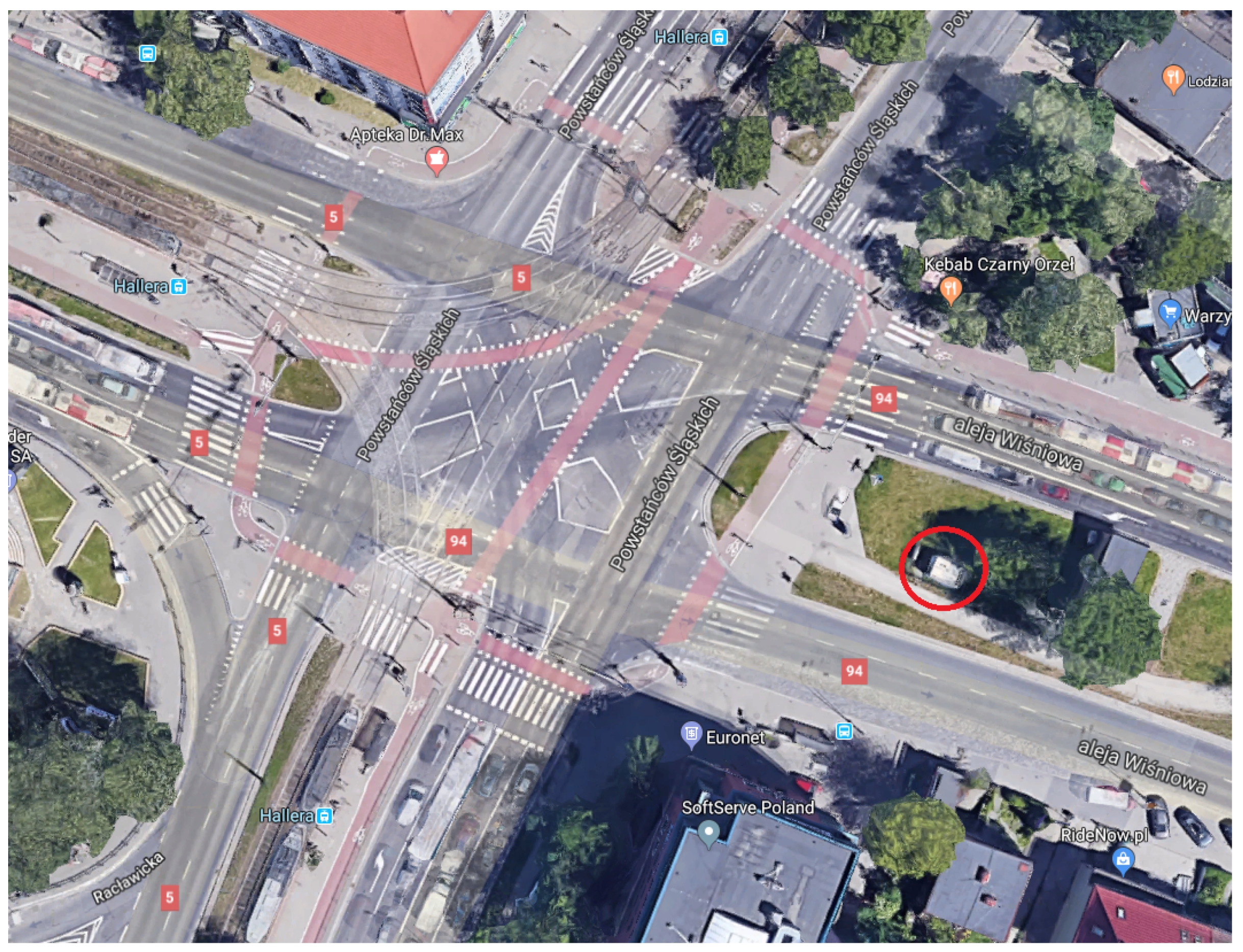
Our purpose in this paper is to solve a temporal regression problem for air quality modelling and prediction. We consider an air quality database that contains measurements of several parameters in the city of Wrocław (Poland); in particular, we consider data from a communication station located within a wide street with two lanes in each direction (GPS coordinates: 51.086390 North, 17.012076 East; see Figure 2). One of the largest intersections in Wrocław is located approximately 30 meters from the measuring station and is covered by traffic monitoring cameras. A weather measurement station is located on the outskirts of the city, at 9.6 km from the airport, and our data set is structured so that all such data are combined in an attempt to predict pollution concentrations. Pollution data are collected by the Provincial Environment Protection Inspectorate and encompasses the hourly NO concentration values during three years, from 2015 to 2017. The traffic data are provided by the Traffic Public Transport Management Department of the Roads and City Maintenance Board in Wrocław and include the hourly count of all types of vehicles passing the intersection. Public meteorological data are provided by the Institute of Meteorology and Water Management, and they include: air temperature, solar duration, wind speed, relative humidity, and air pressure. In order to make the data uniform, solar duration values were re-normalized in the real interval . In the pre-processing phase, the instances with at least one missing value (617 samples, 2.3%) were deleted. Some basic statistic indicators on the remaining 25,687 instances are presented in Table 2.
We considered, in particular, the set that contains the transport, meteorological, and pollution data from the year 2017. From it, we extracted the sets , where ranges from Jan to Dec, each containing the hourly data of the first 10 days of each month. Therefore, each contains exactly 240 instances. For each month, then, we designed a regression experiment using: (i) classic, non-temporal linear regression (using the class LinearRegression); (ii) classic, non-temporal decision tree regression (using the class RepTree); (iii) lagged linear regression on the lagged version of , with ; (iv) lagged propositional decision tree regression on the lagged version of , with , and (v) feature and language selection for temporal decision tree regression on the transformed version of , with and . We tested the prediction capabilities of each of the extracted models on the corresponding set . In the case of temporal regression, each experiment returned a set of classifiers, more precisely a Pareto set; from it, we selected the classifier with the best correlation. All experiments were executed in 10-fold cross-validation mode, which guarantees the reliability of the results. Observe how different experiments correspond, in fact, to different preprocessing of the data: In (i) and (ii), a given contains 240 instances, each corresponding to a specific hour sample, and six (+1) columns, each corresponding to an independent variable (plus the dependent one). In (iii) and (iv), a given contains 60 (+1) columns, each being an independent variable or its lagged version, with lags from one to 10 h; therefore, the number of instances is actually 231 (), because the first sample for which the dependent value can be computed is the one at Hour 10. Finally, in (v), a given contains 231 multivariate time series, each with 10 values of each of the independent variables, temporally ordered, and labelled with the values of the independent one, starting, again, from the sample at Hour 10.
6. Results and Discussion
All results can be seen in the tables from Table 3, Table 4, Table 5 and Table 6, in which we report, per each experiment, not only the correlation coefficient (cc) between the ground truth and the predicted value [20,42,43], but also the mean average error (mae), the root mean squared error (rmse), and the relative absolute error (rae). The first group of results concerns non-lagged data and standard approaches. As we can see, the correlation coefficient ranges from 0.59 to 0.83, with an average of 0.71, in the linear regression models, and from 0.60 to 0.72, with an average of 0.72, in the decision tree models. The fact that the latter show a slightly better behaviour than the former may indicate that the underlying process is not (strongly) linear and that a stepwise function may approximate this reality in a better way. The fact that the average correlation is not too high in both cases and that in both case, there is at least one month in which it is particularly low may indicate that non-lagged data probably do not capture the underlying phenomenon in its full complexity.
As much as lagged data are concerned, in linear regression models, the correlation coefficients range from 0.71 to 0.84, with an average of 0.78, while in decision tree models from 0.65 to 0.87, with an average of 0.76, presented in Table 4. As we can see, the situation reversed itself, the linear models being more precise than the decision tree ones. A possible explanation is that, while lagged data, in general, offer more information about the underlying process, reasoning with more variables (i.e., 60 vs. six) allows finding very complex regression hyperplanes, which adapt to the data in a natural way; unfortunately, this is a recipe for non-interpretability, as having such a complex regression function, with different coefficients for the same independent variable at different lags, makes it very difficult for the expert to create an explanatory physical theory. To give one example, we consider the linear model extracted from and, in particular, the coefficients of each variable, as shown in Table 5. As can be observed, the alleged influence of every variable seems to have some erratic behaviour, with coefficients with different signs and absolute values at different lags. It could be argued that such a matrix of values is no different from a weight matrix of a neural network, in some sense.
Finally, in Table 6, we can see the results of Temporal J48, in which case the correlation coefficient ranges from 0.78 to 0.87, with an average of 0.83. As can be noticed, in exchange for a higher computational experimental complexity, this method returns clearly better results. This is to be expected, as, by its nature, it combines the benefits of the lagged variables with those of symbolic regression. One can observe not only the improvement in the average, but also in the stability among the twelve months: in the worst case, the correlation index is 0.78, which is to be compared, for example, with the worst case of simple linear regression (0.59). Moreover, it seems that Temporal J48 behaves in a particularly good way on difficult cases: if the case of , for example, we have a correlation coefficient of 0.67 with non-lagged data and decision trees, 0.65 with lagged data and decision trees, and 0.78 with serialized data. In addition to the statistical performances of these models, the following aspects should be noticed. First, these models were extracted in a feature selection context; however, in all cases, the evolutionary algorithm found that all variables had some degree of importance, and no variable was eliminated. Second, the language(s) that was selected allows one to draw some considerations on the nature of the problem; for example, the fact that, in all cases, the relation during or its inverse (i.e., or ) was selected indicates that the past interactions between the variables is a key element for modelling this particular phenomenon. Because Temporal J48, in this experiment, was run without pruning, the resulting trees cannot be easily displayed because of their dimensions. Nevertheless, thanks to its intrinsic interpretability, meta-rules can be easily extracted from a regression tree, as, for example:
which can contribute to designing a real-world theory of the modelled phenomenon. The language selection part performed by the optimizer, in general, reduces the set of used temporal operators of HS when extracting the rules (see Table 6), and this is desirable considering that, among many others, one desideratum for interpretability is to explain the reasoning in an understandable way to humans, which have a strong and specific bias towards simpler descriptions [44].
7. Conclusions
In this paper, we consider an air quality modelling problem as an example of the application of a novel symbolic multivariate temporal regression technique. Multivariate temporal regression is the task of constructing a function that explains the behaviour of a dependent variable over time, using current and past values of a set of independent ones; air quality modelling and, in particular, modelling the values of a pollutant as a function of meteorological and car traffic variables can be seen as a multivariate temporal regression problem. Such problems are classically approached with a number of techniques, which range from simple linear regression to recurrent neural networks; despite their excellent statistical performances, in most cases, such models are unsatisfactory in terms of their interpretability and explainability. Classic symbolic regression is an alternative to functional models; unfortunately, symbolic regression has not been very popular, probably due to the fact that its statistical performances tend not to be good enough for many problems. Temporal symbolic regression reveals itself as a promising compromise between the two strategies: while keeping a symbolic nature, temporal symbolic regression takes into account the temporal component of a problem in a native way. In this paper, we not only apply a temporal symbolic regression to a real-world problem, but we also show that it can be embedded into a feature selection strategy enriched with a language selection one. The resulting approach shows an interesting potential, the statistical performances of the extracted models being superior to those of both atemporal and temporal classical approaches.
Author Contributions
Conceptualization, G.S.; Data curation, E.L.-S.; Investigation, G.S. and I.E.S.; Methodology, G.S. and I.E.S.; Project administration, G.S.; Resources, E.L.-S.; Software, E.L.-S. and I.E.S.; Writing—original draft, G.S. and I.E.S. All authors have read and agreed to the published version of the manuscript.
Funding
This research received no external funding.
Data Availability Statement
Not Applicable, the study does not report any data.
Acknowledgments
The authors acknowledge the partial support from the following projects: Artificial Intelligence for Improving the Exploitation of Water and Food Resources, founded by the University of Ferrara under the FIR program, and New Mathematical and Computer Science Methods for Water and Food Resources Exploitation Optimization, founded by the Emilia-Romagna region, under the POR-FSE program.
Conflicts of Interest
The authors declare no conflict of interest.
References
- Holnicki, P.; Tainio, M.; Kałuszko, A.; Nahorski, Z. Burden of mortality and disease attributable to multiple air pollutants in Warsaw, Poland. Int. J. Environ. Res. Public Health 2017, 14, 1359. [Google Scholar] [CrossRef] [Green Version]
- Schwartz, J. Lung function and chronic exposure to air pollution: A cross-sectional analysis of NHANES II. Environ. Res. 1989, 50, 309–321. [Google Scholar] [CrossRef]
- Peng, R.D.; Dominici, F.; Louis, T.A. Model choice in time series studies of air pollution and mortality. J. R. Stat. Soc. Ser. A Stat. Soc. 2006, 169, 179–203. [Google Scholar] [CrossRef] [Green Version]
- Mar, T.; Norris, G.; Koenig, J.; Larson, T. Associations between air pollution and mortality in Phoenix, 1995–1997. Environ. Health Perspect. 2000, 108, 347–353. [Google Scholar] [CrossRef] [PubMed]
- Knibbs, L.; Cortés, A.; Toelle, B.; Guo, Y.; Denison, L.; Jalaludin, B.; Marks, G.; Williams, G. The Australian Child Health and Air Pollution Study (ACHAPS): A national population-based cross-sectional study of long-term exposure to outdoor air pollution, asthma, and lung function. Environ. Int. 2018, 120, 394–403. [Google Scholar] [CrossRef]
- Cifuentes, L.; Vega, J.; Köpfer, K.; Lave, L. Effect of the fine fraction of particulate matter versus the coarse mass and other pollutants on daily mortality in Santiago, Chile. J. Air Waste Manag. Assoc. 2000, 50, 1287–1298. [Google Scholar] [CrossRef]
- Chianese, E.; Camastra, F.; Ciaramella, A.; Landi, T.C.; Staiano, A.; Riccio, A. Spatio-temporal learning in predicting ambient particulate matter concentration by multi-layer perceptron. Ecol. Inform. 2019, 49, 54–61. [Google Scholar] [CrossRef]
- Nieto, P.G.; Lasheras, F.S.; García-Gonzalo, E.; de Cos Juez, F. PM10 concentration forecasting in the metropolitan area of Oviedo (Northern Spain) using models based on SVM, MLP, VARMA and ARIMA: A case study. Sci. Total Environ. 2018, 621, 753–761. [Google Scholar] [CrossRef] [PubMed]
- Gilbert, N.; Goldberg, M.; Beckerman, B.; Brook, J.; Jerrett, M. Assessing spatial variability of ambient nitrogen dioxide in Montreal, Canada, with a land-use regression model. J. Air Waste Manag. Assoc. 2005, 55, 1059–1063. [Google Scholar] [CrossRef] [Green Version]
- Henderson, S.; Beckerman, B.; Jerrett, M.; Brauer, M. Application of land use regression to estimate long-term concentrations of traffic-related nitrogen oxides and fine particulate matter. Environ. Sci. Technol. 2007, 41, 2422–2428. [Google Scholar] [CrossRef]
- Hoek, G.; Beelen, R.; Hoogh, K.D.; Vienneau, D.; Gulliver, J.; Fischer, P.; Briggs, D. A review of land-use regression models to assess spatial variation of outdoor air pollution. Atmos. Environ. 2008, 42, 7561–7578. [Google Scholar] [CrossRef]
- Lucena-Sánchez, E.; Jiménez, F.; Sciavicco, G.; Kaminska, J. Simple Versus Composed Temporal Lag Regression with Feature Selection, with an Application to Air Quality Modeling. In Proceedings of the Conference on Evolving and Adaptive Intelligent Systems, Bari, Italy, 27–29 May 2020; pp. 1–8. [Google Scholar]
- Kaminska, J. A random forest partition model for predicting NO2 concentrations from traffic flow and meteorological conditions. Sci. Total Environ. 2015, 651, 475–483. [Google Scholar] [CrossRef]
- Breiman, L.; Friedman, J.; Olshen, R.; Stone, C. Classification and Regression Trees; Chapman and Hall/CRC: Wadsworth, OH, USA, 1984. [Google Scholar]
- Clark, P.; Niblett, T. The CN2 Induction Algorithm. Mach. Learn. 1989, 3, 261–283. [Google Scholar] [CrossRef]
- Sciavicco, G.; Stan, I. Knowledge Extraction with Interval Temporal Logic Decision Trees. In Proceedings of the 27th International Symposium on Temporal Representation and Reasoning, Bozen-Bolzano, Italy, 23–25 September 2020; Volume 178, pp. 9:1–9:16. [Google Scholar]
- Lucena-Sánchez, E.; Sciavicco, G.; Stan, I. Symbolic Learning with Interval Temporal Logic: The Case of Regression. In Proceedings of the 2nd Workshop on Artificial Intelligence and Formal Verification, Logic, Automata, and Synthesis , Bozen-Bolzano, Italy, 25 September 2020; Volume 2785, pp. 5–9. [Google Scholar]
- Halpern, J.Y.; Shoham, Y. A Propositional Modal Logic of Time Intervals. J. ACM 1991, 38, 935–962. [Google Scholar] [CrossRef]
- Allen, J.F. Maintaining Knowledge about Temporal Intervals. Commun. ACM 1983, 26, 832–843. [Google Scholar] [CrossRef]
- Witten, I.H.; Frank, E.; Hall, M.A. Data Mining: Practical Machine Learning Tools and Techniques, 4th ed.; Morgan Kaufmann: Burlington, MA, USA, 2017. [Google Scholar]
- John, G. Robust Decision Trees: Removing Outliers from Databases. In Proceedings of the 1st International Conference on Knowledge Discovery and Data Mining, Montreal, QC, Canada, 20–21 August 1995; pp. 174–179. [Google Scholar]
- Maronna, R.; Martin, D.; Yohai, V. Robust Statistics: Theory and Methods; Wiley: Hoboken, NJ, USA, 2006. [Google Scholar]
- Box, G.; Jenkins, G.; Reinsel, G.; Ljung, G. Time Series Analysis: Forecasting and Control; Wiley: Hoboken, NJ, USA, 2016. [Google Scholar]
- Guyon, I.; Elisseeff, A. An introduction to variable and feature selection. J. Mach. Learn. Res. 2003, 3, 1157–1182. [Google Scholar]
- Siedlecki, W.; Sklansky, J. A note on genetic algorithms for large-scale feature selection. In Handbook of Pattern Recognition and Computer Vision; World Scientific: Singapore, 1993; pp. 88–107. [Google Scholar]
- Vafaie, H.; Jong, K.D. Genetic algorithms as a tool for feature selection in machine learning. In Proceedings of the 4th Conference on Tools with Artificial Intelligence, Arlington, VA, USA, 10–13 November 1992; pp. 200–203. [Google Scholar]
- ElAlamil, M. A filter model for feature subset selection based on genetic algorithm. Knowl. Based Syst. 2009, 22, 356–362. [Google Scholar] [CrossRef]
- Anirudha, R.; Kannan, R.; Patil, N. Genetic algorithm based wrapper feature selection on hybrid prediction model for analysis of high dimensional data. In Proceedings of the 9th International Conference on Industrial and Information Systems, Gwalior, India, 15–17 December 2014; pp. 1–6. [Google Scholar]
- Huang, J.; Cai, Y.; Xu, X. A hybrid genetic algorithm for feature selection wrapper based on mutual information. Pattern Recognit. Lett. 2007, 28, 1825–1844. [Google Scholar] [CrossRef]
- Yang, J.; Honavar, V. Feature subset selection using a genetic algorithm. IEEE Intell. Syst. Their Appl. 1998, 13, 44–49. [Google Scholar] [CrossRef] [Green Version]
- Jiménez, F.; Sánchez, G.; García, J.; Sciavicco, G.; Miralles, L. Multi-objective evolutionary feature selection for online sales forecasting. Neurocomputing 2017, 234, 75–92. [Google Scholar] [CrossRef]
- Mukhopadhyay, A.; Maulik, U.; Bandyopadhyay, S.; Coello, C.C. A survey of multiobjective evolutionary algorithms for data mining: Part I. IEEE Trans. Evol. Comput. 2014, 18, 4–19. [Google Scholar] [CrossRef]
- Dash, M.; Liu, H. Feature Selection for Classification. Intell. Data Anal. 1997, 1, 131–156. [Google Scholar] [CrossRef]
- Ishibuchi, H.; Nakashima, T. Multi-objective pattern and feature selection by a genetic algorithm. In Proceedings of the Genetic and Evolutionary Computation Conference, Las Vegas, NV, USA, 8–12 July 2000; pp. 1069–1076. [Google Scholar]
- Emmanouilidis, C.; Hunter, A.; Macintyre, J.; Cox, C. A multi-objective genetic algorithm approach to feature selection in neural and fuzzy modeling. Evol. Optim. 2001, 3, 1–26. [Google Scholar]
- Liu, J.; Iba, H. Selecting informative genes using a multiobjective evolutionary algorithm. In Proceedings of the Congress on Evolutionary Computation, Honolulu, HI, USA, 12–17 May 2002; pp. 297–302. [Google Scholar]
- Pappa, G.L.; Freitas, A.A.; Kaestner, C. Attribute selection with a multi-objective genetic algorithm. In Proceedings of the 16th Brazilian Symposium on Artificial Intelligence, Porto de Galinhas/Recife, Brazil, 11–14 November 2002; pp. 280–290. [Google Scholar]
- Shi, S.; Suganthan, P.; Deb, K. Multiclass protein fold recognition using multiobjective evolutionary algorithms. In Proceedings of the Symposium on Computational Intelligence in Bioinformatics and Computational Biology, La Jolla, CA, USA, 7–8 October 2004; pp. 61–66. [Google Scholar]
- Collette, Y.; Siarry, P. Multiobjective Optimization: Principles and Case Studies; Springer: Berlin/Heidelberg, Germany, 2004. [Google Scholar]
- Deb, K. Multi-Objective Optimization Using Evolutionary Algorithms; Wiley: London, UK, 2001. [Google Scholar]
- Durillo, J.; Nebro, A. JMetal: A Java Framework for Multi-Objective Optimization. Av. Eng. Softw. 2011, 42, 760–771. [Google Scholar] [CrossRef]
- Johnson, R.A.; Bhattacharyya, G.K. Statistics: Principles and Methods, 8th ed.; Wiley: Hoboken, NJ, USA, 2019. [Google Scholar]
- James, G.; Witten, D.; Hastie, T.; Tibshirani, R. An Introduction to Statistical Learning: With Applications in R; Springer: Berlin/Heidelberg, Germany, 2013. [Google Scholar]
- Gilpin, L.H.; Bau, D.; Yuan, B.Z.; Bajwa, A.; Specter, M.; Kagal, L. Explaining Explanations: An Overview of Interpretability of Machine Learning. In Proceedings of the IEEE 5th International Conference on Data Science and Advanced Analytics, Turin, Italy, 1–3 October 2018; pp. 80–89. [Google Scholar]
Figure 1.
A multivariate time series with three variables (top). Static regression (middle, left). Static lagged regression (middle, right). Multivariate time series regression (bottom).
Figure 1.
A multivariate time series with three variables (top). Static regression (middle, left). Static lagged regression (middle, right). Multivariate time series regression (bottom).

Figure 2.
An aerial view of the area of interest. The red circle is the communication station.


Table 1.
Allen’s relations and their logical notation. HS, Halpern and Shoham.
| HS Modality | Definition w.r.t. the Interval Structure | Example | ||
|---|---|---|---|---|
| (after) | ⇔ |  | ||
| (later) | ⇔ | |||
| (begins) | ⇔ | |||
| (ends) | ⇔ | |||
| (during) | ⇔ | |||
| (overlaps) | ⇔ | |||
Table 2.
Descriptive statistics.
| Variable | Unit | Mean | St.Dev. | Min | Median | Max |
|---|---|---|---|---|---|---|
| Air temperature | °C | 10.9 | 8.4 | −15.7 | 10.1 | 37.7 |
| Solar duration | h | 0.23 | 0.38 | 0 | 0 | 1 |
| Wind speed | ms | 3.13 | 1.95 | 0 | 3.00 | 19 |
| % relative humidity | − | 74.9 | 17.3 | 20 | 79.0 | 100 |
| Air pressure | hPa | 1003 | 8.5 | 906 | 1003 | 1028 |
| Traffic | − | 2771 | 1795.0 | 30 | 3178 | 6713 |
| NO | μgm | 50.4 | 23.2 | 1.7 | 49.4 | 231.6 |
Table 3.
Test results, non-temporal data: linear regression (top) and decision tree regression (bottom).
Table 3.
Test results, non-temporal data: linear regression (top) and decision tree regression (bottom).
| Month | cc | mae | rmse | rae (%) |
| Jan | 0.75 | 10.47 | 13.38 | 63.61 |
| Feb | 0.73 | 10.67 | 12.86 | 67.86 |
| Mar | 0.65 | 12.66 | 16.04 | 73.62 |
| Apr | 0.68 | 12.05 | 14.62 | 75.87 |
| May | 0.71 | 10.00 | 13.63 | 61.86 |
| Jun | 0.61 | 12.57 | 15.34 | 79.93 |
| Jul | 0.59 | 11.90 | 15.09 | 79.35 |
| Aug | 0.69 | 13.62 | 17.07 | 70.74 |
| Sep | 0.72 | 11.47 | 15.21 | 64.24 |
| Oct | 0.83 | 8.84 | 11.11 | 52.95 |
| Nov | 0.76 | 8.58 | 11.25 | 61.18 |
| Dec | 0.77 | 9.32 | 12.05 | 57.15 |
| average | 0.71 | 11.01 | 12.84 | 67.36 |
| Month | cc | mae | rmse | rae (%) |
| Jan | 0.77 | 9.35 | 13.21 | 56.84 |
| Feb | 0.75 | 9.89 | 12.92 | 62.91 |
| Mar | 0.67 | 12.71 | 16.59 | 73.90 |
| Apr | 0.76 | 9.86 | 13.41 | 62.09 |
| May | 0.71 | 10.34 | 13.99 | 63.97 |
| Jun | 0.70 | 11.24 | 14.58 | 71.45 |
| Jul | 0.67 | 11.21 | 14.87 | 74.74 |
| Aug | 0.76 | 11.87 | 15.96 | 61.63 |
| Sep | 0.60 | 12.88 | 18.82 | 72.13 |
| Oct | 0.76 | 9.74 | 13.35 | 58.37 |
| Nov | 0.74 | 8.91 | 11.93 | 63.58 |
| Dec | 0.75 | 9.55 | 12.93 | 58.55 |
| average | 0.72 | 9.85 | 13.28 | 60.28 |
Table 4.
Test results, lagged data; linear regression (top), and decision-tree regression (bottom).
| Month | cc | mae | rmse | rae (%) |
| Jan | 0.80 | 9.79 | 12.21 | 59.51 |
| Feb | 0.83 | 8.35 | 10.58 | 53.16 |
| Mar | 0.81 | 9.45 | 12.66 | 54.94 |
| Apr | 0.71 | 11.43 | 14.30 | 71.95 |
| May | 0.73 | 10.67 | 13.86 | 66.02 |
| Jun | 0.72 | 10.61 | 13.63 | 67.41 |
| Jul | 0.75 | 9.94 | 12.57 | 66.29 |
| Aug | 0.77 | 12.80 | 15.45 | 66.44 |
| Sep | 0.78 | 11.31 | 14.56 | 63.34 |
| Oct | 0.82 | 9.00 | 11.58 | 53.96 |
| Nov | 0.80 | 8.22 | 10.60 | 58.61 |
| Dec | 0.84 | 8.08 | 10.42 | 49.51 |
| average | 0.78 | 9.09 | 12.70 | 60.93 |
| Month | cc | mae | rmse | rae (%) |
| Jan | 0.75 | 9.59 | 13.75 | 58.31 |
| Feb | 0.84 | 7.93 | 10.41 | 50.43 |
| Mar | 0.78 | 10.26 | 13.42 | 59.65 |
| Apr | 0.71 | 10.29 | 14.45 | 64.75 |
| May | 0.77 | 9.36 | 12.65 | 57.91 |
| Jun | 0.70 | 11.08 | 14.59 | 70.45 |
| Jul | 0.65 | 10.96 | 15.21 | 73.09 |
| Aug | 0.75 | 12.10 | 16.19 | 62.84 |
| Sep | 0.78 | 10.09 | 14.01 | 56.49 |
| Oct | 0.75 | 10.12 | 13.98 | 60.67 |
| Nov | 0.79 | 7.83 | 10.74 | 55.85 |
| Dec | 0.87 | 7.11 | 9.54 | 43.61 |
| average | 0.76 | 8.87 | 13.24 | 54.11 |
Table 5.
Test results, lagged data: coefficients for the linear regression, January.
| Variable | Lag | |||||||||
|---|---|---|---|---|---|---|---|---|---|---|
| Air temperature | −0.77 | −0.50 | 0.00 | −1.14 | 0.00 | 0.00 | 0.00 | 0.93 | 0.00 | 0.00 |
| Sol.duration | 0.00 | 0.00 | 0.00 | 7.36 | 0.00 | 7.26 | 0.00 | 0.00 | 0.00 | 0.00 |
| Wind speed | −2.006 | −2.50 | −1.85 | 7.36 | 0.00 | −1.14 | 0.00 | 0.00 | 0.00 | −1.08 |
| Rel.humidity | −0.29 | −0.19 | −0.23 | −0.22 | 0.00 | 0.00 | 0.29 | 0.00 | 0.21 | 0.00 |
| Air pressure | 0.00 | 1.97 | −2.25 | 0.00 | 0.00 | −2.47 | 0.71 | 0.48 | −1.21 | 1.59 |
| Traffic | −0.82 | −0.22 | 0.43 | −0.32 | 0.45 | −0.28 | 0.00 | 0.00 | 0.00 | 0.00 |
Table 6.
Test results, temporal decision tree regression.
| Month | cc | mae | rmse | rae (%) | Language |
|---|---|---|---|---|---|
| Jan | 0.87 | 7.73 | 10.54 | 46.91 | |
| Feb | 0.86 | 7.39 | 9.70 | 47.65 | |
| Mar | 0.79 | 10.73 | 13.93 | 63.41 | |
| Apr | 0.85 | 7.77 | 10.86 | 48.57 | |
| May | 0.84 | 7.87 | 10.53 | 50.52 | |
| Jun | 0.82 | 9.07 | 11.60 | 58.00 | |
| Jul | 0.78 | 10.00 | 12.87 | 65.62 | |
| Aug | 0.83 | 10.82 | 13.90 | 55.97 | |
| Sep | 0.81 | 9.50 | 13.17 | 53.77 | |
| Oct | 0.81 | 9.31 | 12.42 | 55.58 | |
| Nov | 0.80 | 8.34 | 11.04 | 61.27 | |
| Dec | 0.85 | 7.31 | 10.47 | 45.10 | |
| average | 0.83 | 8.82 | 11.75 | 54.36 |
Publisher’s Note: MDPI stays neutral with regard to jurisdictional claims in published maps and institutional affiliations. |
© 2021 by the authors. Licensee MDPI, Basel, Switzerland. This article is an open access article distributed under the terms and conditions of the Creative Commons Attribution (CC BY) license (http://creativecommons.org/licenses/by/4.0/).
Share and Cite
MDPI and ACS Style
Lucena-Sánchez, E.; Sciavicco, G.; Stan, I.E. Feature and Language Selection in Temporal Symbolic Regression for Interpretable Air Quality Modelling. Algorithms 2021, 14, 76. https://0-doi-org.brum.beds.ac.uk/10.3390/a14030076
AMA Style
Lucena-Sánchez E, Sciavicco G, Stan IE. Feature and Language Selection in Temporal Symbolic Regression for Interpretable Air Quality Modelling. Algorithms. 2021; 14(3):76. https://0-doi-org.brum.beds.ac.uk/10.3390/a14030076
Chicago/Turabian StyleLucena-Sánchez, Estrella, Guido Sciavicco, and Ionel Eduard Stan. 2021. "Feature and Language Selection in Temporal Symbolic Regression for Interpretable Air Quality Modelling" Algorithms 14, no. 3: 76. https://0-doi-org.brum.beds.ac.uk/10.3390/a14030076
Note that from the first issue of 2016, this journal uses article numbers instead of page numbers. See further details here.