
On the Descriptive Complexity of Color Coding †


Institute for Theoretical Computer Science, Universität zu Lübeck, 23562 Lübeck, Germany
*
Authors to whom correspondence should be addressed.
†
This paper is an extended version of our paper published in STACS 2019.
Algorithms 2021, 14(3), 96; https://0-doi-org.brum.beds.ac.uk/10.3390/a14030096
Submission received: 29 January 2021
/
Revised: 13 March 2021
/
Accepted: 16 March 2021
/
Published: 19 March 2021
(This article belongs to the Special Issue Parameterized Complexity and Algorithms for Nonclassical Logics)
Abstract
:Color coding is an algorithmic technique used in parameterized complexity theory to detect “small” structures inside graphs. The idea is to derandomize algorithms that first randomly color a graph and then search for an easily-detectable, small color pattern. We transfer color coding to the world of descriptive complexity theory by characterizing—purely in terms of the syntactic structure of describing formulas—when the powerful second-order quantifiers representing a random coloring can be replaced by equivalent, simple first-order formulas. Building on this result, we identify syntactic properties of first-order quantifiers that can be eliminated from formulas describing parameterized problems. The result applies to many packing and embedding problems, but also to the long path problem. Together with a new result on the parameterized complexity of formula families involving only a fixed number of variables, we get that many problems lie in FPT just because of the way they are commonly described using logical formulas.
1. Introduction
Descriptive complexity provides a powerful link between logic and complexity theory: We use a logical formula to describe a problem and can then infer the computational complexity of the problem just from the syntactic structure of the formula. As a striking example, Fagin’s Theorem [1] tells us that 3-colorability lies in NP just because its describing formula (“there exist three colors such that all adjacent vertex pairs have different colors”) is an existential second-order formula. In the context of fixed-parameter tractability theory, methods from descriptive complexity are also used a lot—but commonly to show that problems are difficult. For instance, the A- and W-hierarchies are defined in logical terms [2], but their hard problems are presumably “beyond” the class FPT of fixed-parameter tractable problems.
The methods of descriptive complexity are only rarely used to show that problems are in FPT. More precisely, the syntactic structure of the natural logical descriptions of standard parameterized problems found in textbooks are not known to imply that the problems lie in FPT—even though this is known to be the case for many of them. To appreciate the underlying difficulties, consider the following three parameterized problems (the prefix “p” stand for “parameterized” and its index names the parameter): , , and . In each case, we are given an undirected graph as input and a number k and we are then asked whether the graph contains k vertex-disjoint edges (a size-k matching), k vertex-disjoint triangles, or a clique of size k, respectively. The problems are known to have widely different complexities (maximal matchings can actually be found in polynomial time, triangle packing lies at least in FPT, while finding cliques is -complete) but very similar logical descriptions:
The family of formulas is clearly a natural “slicewise” description of the matching problem: A graph has a size-k matching if and only if . The families and are natural parameterized descriptions of the triangle packing and the clique problems, respectively. Well-known results on the descriptive complexity of parameterized problems allow us to infer [2] from the above descriptions that all three problems lie in , but offer no hint why the first two problems actually lie in the class FPT—syntactically the clique problem arguably “looks like the easiest one” when in fact it is semantically the most difficult one. The results of this paper will remedy this mismatch between syntactic and semantic complexity: We will show that the syntactic structures of the formulas and imply membership of and in FPT. In particular, we will identify the non-obvious syntactic properties that make and “easier” than .
The road to deriving the computational complexity of parameterized problems just from the syntactic properties of slicewise first-order descriptions involves three major steps: First, a characterization of when the color coding technique is applicable in terms of syntactic properties of second-order quantifiers. Second, an exploration of how these results on second-order formulas apply to first-order formulas, leading to the notion of strong and weak quantifiers and to an elimination theorem for weak quantifiers. Third, we add a new characterization to the body of known characterizations of how classes like FPT can be characterized in a slicewise fashion by logical formulas.
- Our Contributions I: A Syntactic Characterization of Color Coding.
Consider once more the triangle packing problem, where we are asked whether an undirected graph G contains k vertex-disjoint triangles. While this problem is known to be hard, it becomes almost trivial if we change it slightly: Suppose someone colored the vertices of the graph and our job is just to determine whether there are a red triangle, a green triangle, a blue triangle, a yellow triangle, and so on for k different colors. Clearly, this is a now a very easy problem and if we do, indeed, find k triangles having k different colors, we have found k vertex-disjoint triangles.
The ingenious idea behind the color coding technique of Alon, Yuster, and Zwick [3] is to reduce the hard triangle packing problem to the much simpler colored version by simply randomly coloring the graph. Of course, even if there are k disjoint triangles, we will most likely not color them monochromatically and differently, but the probability of “getting lucky” is nonzero (at least ) and depends only on the parameter k. Even better, Alon et al. point out that one can derandomize the coloring easily by using universal hash functions to color each vertex with its hash value.
Applying this idea in the setting of descriptive complexity was recently pioneered by Chen et al. [4]. Transferred to the triangle packing problem, their argument would roughly be: “Testing for each color i, whether there is a monochromatic triangle of color i, can be done in first-order logic using something like . Next, instead of testing whether x has color i using the formula , we can test whether x gets hashed to i by a hash function. Finally, since computing appropriate universal hash functions only involves addition and multiplication, we can express the derandomized algorithm using an arithmetic first-order formula of low quantifier rank.” Phrased differently, Chen et al. would argue that together with the requirement that the are pairwise disjoint is (ignoring some details) equivalent to , where is a formula that is true when “x is hashed to i by a member of a universal family of hash functions indexed by q and p.”
The family may seem rather technical and, indeed, its importance becomes visible only in conjunction with another result by Chen et al. [4]: They show that a parameterized problem lies in , one of the smallest “sensible” subclasses of FPT, if it can be described by a family of formulas of bounded quantifier rank such that the finite models of are exactly the elements of the kth slice of the problem. Since the triangle packing problem can be described in this way via the family of formulas, all of which have a quantifier rank 5 plus the constant number of quantifiers used to express the arithmetics in the formulas , we get .
Clearly, this beautiful idea cannot work in all situations: If it also worked for the formula mentioned earlier expressing 3-colorability, 3-colorability would be first-order expressible, which is known to be impossible. Our first main contribution is a syntactic characterization of when the color coding technique is applicable, that is, of why color coding works for triangle packing but not for 3-colorability: For triangle packing, the colors are applied to variables only inside existential scopes (“”) while for 3-colorability the colors R, G, and B are also applied to variables inside universal scopes (“for all adjacent vertices”). In general, see Theorem 2 for the details, we show that a second-order quantification over an arbitrary number of disjoint colors can be replaced by a fixed number of first-order quantifiers whenever none of the is used in a universal scope.
- Our Contributions II: New First-Order Quantifier Elimination Rules.
The “purpose” of the colors in the formulas is not that the three vertices of a triangle get a particular color, but just that they get a color different from the color of all other triangles. Indeed, our “real” objective in these formulas is to ensure that the vertices of a triangle are distinct from the vertices in the other triangles—and giving vertices different colors is “just a means” of ensuring this.
In our second main contribution we explore this idea further: If the main (indeed, the only) use of colors in the context of color coding is to ensure that certain vertices are different, let us do away with colors and instead focus on the notion of distinctness. To better explain this idea, consider the following family, also describing triangle packing, where the only change is that we now require (a bit superfluously) that even the vertices inside a triangle get different colors: . Observe that each is now applied to exactly one variable (x, y, or z in one of the many literals) and the only “effect” that all these applications have is to ensure that the vertices to which these variables get bound are different. In particular, the formula is equivalent to
and these formulas are clearly equivalent to the almost identical formulas from (2).
In a sense, in (4) the many existential quantifiers and the many literals come “for free” from the color coding technique, while , , and have nothing to do with color coding. Our key observation is a syntactic property that tells us whether a quantifier comes “for free” in this way (we will call it weak) or not (we will call it strong): Definition 3 states (essentially) that weak quantifiers have the form such that x is not free in any universal scope of and x is used in at most one literal that is not of the form . To make weak quantifiers easier to spot, we mark the variables they bind with a dot (note that this is just a “syntactic hint to the reader” without any semantic meaning). Formulas (4) now read . Observe that x, y, and z are not weak since each is used in three literals that are not inequalities.
We show in Theorem 4 that each is equivalent to a whose quantifier rank depends only on the strong quantifier rank of (meaning that we ignore the weak quantifiers) and whose number of variables depends only on the number of strong variables in . For instance, the formulas from (4) all have strong quantifier rank 3 and, thus, the triangle packing problem can be described by a family of constant (normal) quantifier rank. Applying Chen et al.’s characterization yields membership in .
As a more complex example, let us sketch a “purely syntactic” proof of the result [5,6] that the embedding problem for graphs H of tree depth at most d lies in for each d. Once more, we construct a family of formulas, one for each to-be-embedded graph H, of constant strong quantifier rank that describes the problem. For a graph to have tree depth d means that there is a rooted tree T of depth d such that is contained in the edges of T’s transitive closure. Let be the root of T and let be the (possibly empty) set of children of c in T. Then the following formula of strong quantifier rank d describes that H can be embedded into a graph structure (note that in the formula the E in “” refers to the edge relation of while in “” it refers to the edge set of the fixed parameter H):
- Our Contributions III: Slicewise Descriptions and Variable Set Sizes.
Our third contribution is a new result in the same vein as the already repeatedly mentioned result of Chen et al. [4], stated as Fact 1 in our paper: Our new Theorem 1 states that a parameterized problem can be described slicewise by a family of arithmetic first-order formulas that all use only a bounded number of variables if and only if the problem lies in —a class that has been encountered repeatedly in the literature [5,7,8,9], but for which no characterization was known. It contains all parameterized problems that can be decided by AC-circuits whose depth depends only on the parameter and whose size is of the form .
As an example, consider the problem of deciding whether a graph contains a path of length k (no vertex may be visited twice). It can be described by the family of formulas with (for odd k) equal to
Note that the strong quantifier rank of is and, thus, depends on k. However, there are only four strong variables, namely s, t, x, and y. By Theorem 3 we see that the above formulas are equivalent to a family of formulas with a bounded number of variables and by Theorem 1 we see that . These ideas also generalize easily and we give a purely syntactic proof of the seminal result from the original color coding paper [3] that the embedding problem for graphs of bounded tree width lies in FPT. The core observation—which unifies the results for tree width and depth—is that for each graph with a given tree decomposition, the embedding problem can be described by a formula whose strong nesting structure mirrors the tree structure and whose strong variables mirror the bag contents.
Table 1 summarizes, for the problems discussed in this paper, how they can be described using formulas in such a way that membership in and follows. All memberships were previously known, the contribution of this paper is that we prove the memberships by presenting families of first-order formulas that describe them, such that that strong quantifier rank (strong-qr) or the number of strong variables (strong-vars) is parameter-independent.
1.1. Related Work
Flum and Grohe [10] were the first to give characterizations of FPT and of many subclasses in terms of the syntactic properties of formulas describing their members. Unfortunately, these syntactic properties do not hold for the descriptions of parameterized problems found in the literature. For instance, they show that FPT contains exactly the problems that can be described by families of -formulas of bounded quantifier rank—but actually describing problems like in this way is more or less hopeless and yields little insights into the structure or complexity of the problem. We believe that it is no coincidence that no applications of these beautiful characterizations to concrete problems could be found in the literature—at least prior to very recent work by Chen and Flum [11], who study slicewise descriptions of problems on structures of bounded tree depth, and the already cited article of Chen et al. [4], who do present a family of formulas that describe the vertex cover problem. This family internally uses the color coding technique and is thus closely related to our results. The crucial difference is, however, that we identify syntactic properties of logical formulas that imply that the color coding technique can be applied. It then suffices to find a family describing a given problem that meets the syntactic properties to establish the complexity of the problem: there is no need to actually construct the color-coding-based formulas—indeed, there is not even a need to understand how color coding works in order to decide whether a quantifier is weak or strong.
A different approach towards proving that a problem lies in FPT purely because of the syntactic nature of logic-based problem descriptions comes from the context of optimization problems. Cai and Chen [12] have shown that all problems in the syntactically-defined classes MAXSNP, due to [13], and , due to [14], are fixed-parameter tractable (but not necessarily in the small classes like and studied in the present paper).
1.2. Organization of this Paper
In Section 2 we first review some of the existing work on the descriptive complexity of parameterized problems. We add to this work in the form of the mentioned characterization of the class in terms of a bounded number of variables. Our main technical results are then proved in Section 3, where we establish and prove the syntactic properties that formulas must have in order for the color coding method to be applicable. In Section 4 we then apply the findings and show how membership of different natural problems in and (and, thus, in FPT) can be derived entirely from the syntactic structure of the formulas describing them.
2. Describing Parameterized Problems
A happy marriage of parameterized complexity and descriptive complexity was first presented in [10] by Flum and Grohe. We first review their most important definitions and then prove a new characterization, namely of the class that contains all problems decidable by AC-circuits of parameter-dependent depth and “FPT-like” size.
2.1. Logical Terminology
We only consider first-order logic and use standard notations following for instance [10], with the perhaps only deviations being that we write relational atoms briefly as instead of and that the literal is an abbreviation for (recall that a literal is an atom or a negated atom). Signatures, typically denoted , are always finite and may only contain relation symbols and constant symbols—with one exception: The special unary function symbol SUCC may also be present in a signature. Let us write for the k-fold application of SUCC, so is short for . It allows us to specify any fixed non-negative integer without having to use additional variables. An alternative is to dynamically add constant symbols for numbers to signatures as done in [4], but we believe that following [10] and adding the successor function gives a leaner formal framework. Let be the maximum arity of relation symbols in .
We denote by the class of all -structures and by the universe of . As is often the case in descriptive complexity theory, we only consider ordered structures in which the ternary predicates ADD and MULT are available and have their natural meaning. Formally, we say is arithmetic if it contains all of the predicates <, ADD, MULT, the function symbol SUCC, and the constant symbol 0 (it is included for convenience only). In this case, contains only those for which is a linear ordering of and the other operations have their natural meaning relative to (with the successor of the maximum element of the universe being itself and with 0 being the minimum with respect to ). We write when is a -formula for an arithmetic .
A -problem is a set closed under isomorphisms. A -formula describes a -problem Q if and it describes Q eventually if describes a set that differs from Q only on structures of a certain maximum size.
Lemma 1.
For each that describes a τ-problem Q eventually, there are quantifier-free formulas α and β such that describes Q.
Proof.
The statement of the lemma would be quite simple if we did not require and to be quantifier-free: Without this requirement, all we need to do is to use and to fix on the finitely many (up to isomorphisms) structures on which errs by “hard-wiring” which of these structures are elements of Q and which are not. However, the natural way to do this “hard-wiring” of size-m structures is to use m quantifiers to bind all elements of the universe. This is exactly what we do not wish to do. Rather, we use the successor function to refer to the elements of the universe without using any quantifiers.
In detail, let m be a number such that for all with (that is, the size of the universe is at least m) we have if and only if . We set to , a shorthand for , which is true only for universes of size at least m. We define so that it is true exactly for all -structures of size at most m (for simplicity we assume that is the only relation symbol in ):
The first line of checks whether the universe of the current structure (the structure for which we would like to know whether it is a model of ) has size s for some and, if so, checks that there is some of size exactly s so that the edges of are present in the current structure (second line) and that the edges not in are also not present in the current structure (last line). In particular, if the current structure has size at most m, it will be a model of if and only if it is isomorphic to some and, thus, if it is an element of Q. □
We write for the quantifier rank of a formula and for the set of its bound variables. For instance, for we have , since the maximum nesting is caused by the two nested existential quantifiers, and .
Let us say that is in negation normal form if negations are applied only to atomic formulas.
2.2. Describing Parameterized Problems
When switching from classical complexity theory to descriptive complexity theory, the basic change is that “words” get replaced by “finite structures.” The same idea works for parameterized complexity theory and, following Flum and Grohe [10], let us define parameterized problems as subsets where Q is closed under isomorphisms. In a pair the number k is, of course, the parameter value of the pair. Flum and Grohe now propose to describe such problems slicewise using formulas. Since this will be the only way in which we describe problems, we will drop the “slicewise” in the phrasings and just say that a family of formulas describes a problem if for all we have if and only if . (In this paper, we ignore the question of whether the mappings should be required to be computable. While this will be the case for all of our examples and constructions, it is not important for our formalism and results.)
For a class of families , let us write for the class of all parameterized problems that are described by the members of (we chose “X” to represent a “slicewise” description, which seems to be in good keeping with the usual use of X in other classes such as XP or XL). For instance, the mentioned characterization of FPT in logical terms by Flum and Grohe can be written as
We remark that instead of describing parameterized problems using families, a more standard and at the same time more flexible way is to use reductions to model checking problems. Clearly, if a family of -formulas describes , then there is a very simple parameterized reduction from Q to the model checking problem , where the input is a pair and the question is whether both and hold. (The function num encodes mathematical objects like or later tuples like as unique natural numbers.) The reduction simply maps a pair to . Even more interestingly, without going into any of the technical details, it is also not hard to see that as long as a reduction is sufficiently simple, the reverse implication holds, that is, we can replace a reduction to the model checking problem by a family of formulas that describe the problem. We can, thus, use whatever formalism seems more appropriate for the task at hand and—as we hope that this paper shows—it is sometimes quite natural to write down a family that describes a problem.
2.3. Parameterized Circuits
For our descriptive setting, we need to slightly adapt the definition of the circuit classes and from [5,7]: Let us say that a problem is in , if there is a family of AC-circuits (Boolean circuits with unbounded fan-in) such that for all we have
- if and only if where x is a binary encoding of and is the length of the encoding,
- the size of each is at most for some function f and some constant c that is independent of both n and k,
- the depth of each is bounded by some constant that is again independent of both n and k, and
- the circuit family satisfies a dlogtime-uniformity condition. (Since the complex questions around circuit uniformity are not of special importance for the present paper, we keep its discussion short and just remark that dlogtime-uniformity roughly means that arithmetic formulas suffice to describe the circuits.)
The class is defined the same way, but the depth may be for some g instead of only . The following fact and theorem show how these two circuit classes are closely related to descriptions of parameterized problems using formulas:
Fact 1
([4]). .
Theorem 1.
.
Proof.
The basic idea behind the proof is quite “old.” We wish to establish links between circuit depth and size and the number of variables used in a formula—and such links are well-known, see for instance [15]: The quantifier rank of a first-order formula naturally corresponds to the depth of a circuit that solves the model checking problem for the formula. The number of variables corresponds to the exponent of the polynomial that bounds the size of the circuit (the paper [16] is actually entitled “”). One thing that is usually not of interest (because only one formula is usually considered) is the fact that the length of the formula is linked multiplicatively to the size of the circuit.
In detail, suppose we are given a problem with via a circuit family of depth and size . For a fixed k, we now need to construct a formula that correctly decides the k-th slice. In other words, we need an -formula whose finite models are exactly those on which the family (note that k no longer indexes the family) evaluates to 1 (when the models are encoded as bitstrings). It is well-known how such a formula can be constructed, see for instance [15], we just need a closer look at how the quantifier rank and number of variables relate to the circuit depth and size.
The basic idea behind the formula is the following: The circuit has gates and we can “address” these gates using c variables (which gives us possibilities) plus a number (which gives us possibilities). Since for fixed k the number is also fixed, it is permissible that the formula contains copies of some subformula, where each subformula handles another value of i. The basic idea is then to start with formulas for , each of which has c free variables, so that is true exactly if the tuple represents an input gate set to 1. At this point, the uniformity condition basically tells us that arithmetic formulas suffice to express this and that they all have a fixed quantifier rank. Next, we construct formulas that are true if addresses a gate for which the input values are all already computed by the and that evaluates to 1. Next, formulas are constructed, but now, we can reuse the variables used in the . In this way, we finally build formulas and apply it to the “address” of the output gate. All told, we get a formula whose quantifier rank is and in which at most variables are used (note that the size of the formula depends on ). Clearly, this means that the family created in this way does, indeed, only use a bounded number of variables (namely many) and decides Q.
For the other direction, suppose describes Q and that all contain at most v variables (since they contain no free variables, this is same as the number of bound variables). Clearly, we may assume that the formulas are in negation normal form. We may also assume that they are “flat,” by which we mean that they contain no subformulas of the form or : Using the distributive laws of propositional logic, any first-order formula can be turned into an equivalent flat formula with the same number of variables and the same quantifier rank (one can loosely think of this as locally transforming the formula into disjunctive normal form, but “not past quantifiers”). Lastly, we may assume that the SUCC function symbol is only used in atoms of the form for some variable x and some number s: We can replace for instance by the equivalent formula without raising the number of variables and the quantifier rank by more than 4 (or, in general, by more than the constant ).
As before, it is now known that for each there is a family that evaluates to 1 exactly on the (encoded) models of . These circuits are constructed as follows: While has no free variables, a subformula of can have up to v free variables. For each such subformula, the circuits use gates to keep track of all assignments to these v variables that make the subformula true. Clearly, this is relatively easy to achieve for literals in a constant number of layers, including literals of the form since s is a fixed number depending only on k. Next, if a formula is of the form and for some assignment we have one gate for each that tells us whether it is true, we can feed all these wires into one ∧-gate. We can take care of a formula of the form in the same way—and note that in a flat formula there will be at most one alternation from ⋀ to ⋁ before we encounter a quantifier. Now, for subformulas of the form , the correct values for the gates can be obtained by a big ∨-gate attached to the outputs from the gates for . Similarly, can be handled using a big ∧-gate.
Based on these observations, it is now possible to build a circuit of size and depth . In particular, the resulting overall circuit family has a depth that depends only on the parameter (since the quantifier rank can be at most , which depends only on k) and has a size of at most for . It can also be shown that the necessary uniformity conditions are satisfied.
We remark that the above proof also implies Fact 1, namely for for the first direction and for for the second direction. □
2.4. Bounded Rank Reductions
To complete the formal framework for describing parameterized problems, we need a notion of parameterized reductions that is very weak to ensure that the smallest class we study, , is closed under them. Such a reduction is used in the literature [5], boringly named -reduction, but both its definition as well as the definition of other kinds of parameterized reductions found in the literature do not fit well with our logical framework: The reductions are defined in terms of machines or circuits that get as input a string that explicitly or implicitly contains the parameter k and output a new problem instance that once more explicitly or implicitly contains a new parameter value .
In contrast, in our setting the inputs and outputs must be logical structures that we wish to define in terms of formulas. Furthermore, “outputting a parameter value” is difficult in our formal framework since parameter values are not elements of the universe, but indices of the formulas. All of these problems can be circumvented, see for instance ([11], Definition 5.3), but we believe it gives a cleaner formalism to give a new “purely logical” definition of reductions between parameterized problems. We will not prove this, but remark that the power of this reduction is the same as that of -reductions.
Definition 1.
Let τ and be signatures and let and be two problems. A bounded rank reduction from Q to , written , is a pair of families and where
- each is a first-order query from τ-structures to -structures and
- each is a τ-formula
such that
- 1.
- for each there is exactly one , denoted by in the following, such that ,
- 2.
- there is a mapping such that for all we have ,
- 3.
- if and only if , and
- 4.
- the quantifier rank of all and of all formulas inside the and of the widths of each is bounded by a constant c.
Let us briefly explain the ingredients of this definition: Each maps all -structures to -structures . The fact that we have one function for each parameter value allows us to make our mapping depend on the parameter. The job of the formulas is solely to “compute” the new parameter value , based not only on the original value k, but also on . If, as is the case in many reductions, the new parameter value just depends on k (typically, it even is k), we can just set to a trivial tautology ⊤ and all other to the contradiction ⊥.
In the definition, we referred to first-order queries, which are a standard way of defining a logical -structure in terms of a -structure in database theory and finite model theory (we remark that in general model theory “interpretation” is used instead of “query” and that “transductions” from fpt-theory are queries with special semantic and syntactic properties). A detailed account of first-order queries can be found in [17], but here is the basic idea: Suppose we wish to map graphs (-structures) to their underlying undirected graphs (-structures, where U represent the underlying symmetric edge set). In this case, there is a simple formula that tells us when holds in the new structure: . More importantly, if we have a formula that internally uses to check whether there is an undirected edge in the mapped graph, we can easily turn this into a formula , where we replace all occurrences of by , that gives the same answer as when fed the original graph. In other words, if a first-order query maps to and we wish to check whether holds, we can just as well check whether holds. The just-described example of a first-order query did not change the universe, which is something we sometimes wish to do. This is achieved by allowing the width w of the query to be larger than 1. The effect is that the universe U gets replaced by and, now, elements of this new universe can be described by tuples of variables of length w. We can also reduce the size of the universe using a formula that is true only for the tuples we wish to keep in the new structure’s universe.
Lemma 2.
Let via a bounded rank reduction given by and . Let describe . Then there is a family that describes Q with
- 1.
- and
- 2.
- .
In particular, and are closed under bounded rank reductions.
Proof.
Set to . By definition, we have if and only if for the unique with . If we can argue that the substitutions do not increase the quantifier rank or number of variables by more than a constant, we get the claim. Unfortunately, there is a case where simple substitutions fail to preserve the quantifier rank, namely when a formula contains a large number of nested applications of the successor function. Suppose, for instance, is something like . While this formula has quantifier rank 2 and uses only two variables, a simple substitution of each occurrence of the one thousand SUCC operators in by any nontrivial formula in that describes the successor function will yield a quantifier rank of at least 1000.
The trick is to use the results from the next section: We can easily modify any formula so that all occurrences of the successor function are of the form for some number i. This means that we “only” need a way of identifying the ith element of the new universe using a bounded quantifier rank. However, assuming for simplicity a width of 1 and assuming that and describe how restricts and reorders the universe, respectively, the formula is true exactly for the ith element of the universe. We will see in the next section that we can express the quantifier using a constant quantifier rank that is independent of i. □
3. Syntactic Properties Allowing Color Coding
The color coding technique [3] is a powerful method from parameterized complexity theory for “discovering small objects” in larger structures. Recall the example from the introduction: While finding k disjoint triangles in a graph is difficult in general, it is easy when the graph is colored with k colors and the objective is to find for each color one triangle having this color. The idea behind color coding is to reduce the (hard) uncolored version to the (easy) colored version by randomly coloring the graph and then “hoping” that the coloring assigns a different color to each triangle. Since the triangles are “small objects,” the probability that they do, indeed, get different colors depends only on k. Even more importantly, Alon et al. noticed that we can derandomize the coloring procedure simply by coloring each vertex by its hash value with respect to a simple family of universal hash functions that only use addition and multiplication [3]. This idea is beautiful and works surprisingly well in practice [18], but using the method inside proofs can be tricky: One needs to “keep the set sizes under control” (they must stay roughly logarithmic in size) and one needs to algorithmically “identify the small set based just on its random coloring,” which especially for more complex proofs can lead to rather subtle arguments.
In the present section, we identify syntactic properties of formulas that guarantee that the color coding technique can be applied. The property is that the colors (the predicates in the formulas) are not in the scope of a universal quantifier (this restriction is necessary, as the example of the formula describing 3-colorability shows).
As mentioned already in the introduction, the main “job” of the colors in proofs based on color coding is typically to ensure that vertices of a graph are different from other vertices. This leads us to the idea of focusing entirely on the notion of distinctness in the second half of this section. This time, there will be syntactic properties of existentially bounded first-order variables that will allow us to apply color coding to them.
3.1. Formulas with Color Predicates
In graph theory, a coloring of a graph can either refer to an arbitrary assignment that maps each vertex to a color or to such an assignment in which vertices connected by an edge must get different colors (sometimes called proper colorings). For our purposes, colorings need not be proper and are thus partitions of the vertex set into color classes. From the logical point of view, each color class can be represented by a unary predicate. A k-coloring of a -structure is a structure over the signature , where the are fresh unary relation symbols, such that is the -restriction of and such that the sets to form a partition of the universe of .
Let us now formulate and prove the first syntactic version of color coding. An example of a possible formula in the below theorem is , for which the theorem tells us that there is a formula of constant quantifier rank that is true exactly when there are pairwise disjoint sets that make true.
Theorem 2.
Let τ be an arithmetic signature and let k be a number. For each first-order -sentence ϕ in negation normal form in which no is inside a universal scope, there is a τ-sentence such that:
- 1.
- For all we have if and only if there is a k-coloring of with .
- 2.
- .
- 3.
- .
(Let us clarify that represents a global constant that is independent of and k.)
Proof.
Let , k, and be given as stated in the theorem. If necessary, we modify to ensure that there is no literal of the form , by replacing each such literal by the equivalent . After this transformation, the in are neither in the scope of universal quantifiers nor of negations—and this is also true for all subformulas of . We will now show by structural induction that all these subformulas (and, hence, also ) have two semantic properties, which we call the monotonicity property and the small witness property (with respect to the ). Afterwards, we will show that these two properties allow us to apply the color coding technique.
Establishing the monotonicity and small witness properties. Some notations will be useful: Given a -structure with universe A and given sets for , let us write to indicate that is a model of where is the -structure with universe A in which all symbols from are interpreted as in and in which the symbol is interpreted as , that is, . Subformulas of may have free variables and suppose that to are the free variables in and let for . We write to indicate that holds in the just-described structure when each is interpreted as .
Definition 2.
Let γ be a -formula with free variables to . We say that γ has the monotonicity and the small witness properties with respect to the if for all τ-structures with universe and all values the following holds:
- 1.
- Monotonicity property: Let and be sets with for all . Then implies .
- 2.
- Small witness property: If there are sets such that we have , then there are sets whose sizes depend only on γ for , such that .
We now show that has these two properties. For monotonicity, just note that the are not in the scope of any negation and, thus, if some make true, so will all supersets of the .
To see that the small witness property holds, we argue by structural induction: If is any formula that does not involve any , then is true or false independently of the and, in particular, if it is true at all, it is also true for for . If is the atomic formula , then setting and for makes the formula true.
If , then and have the small witness property by the induction hypothesis. Let make hold in . Then they also make both and hold in . Let with be the witnesses for and let be the witnesses for . Then by the monotonicity property, makes both and true, that is
and the same holds for . Note that still holds and that they have sizes depending only on and and thereby on .
For we can argue in exactly the same way as for the logical and.
The last case for the structural induction is . Consider that make true. Then there is a value such that . Now, since has the small witness property by the induction hypothesis, we get of size depending on for which we also have . Then, by the definition of existential quantifiers, these also witness . (Observe that this is the point where the argument would not work for a universal quantifier: Here, for each possible value of we might have a different set of ’s as witnesses and their union would then no longer have small size.)
Applying color coding: our next step in the proof is to use color coding to produce the partition. First, let us recall the basic lemma on universal hash functions formulated below in a way equivalent to ([2], p. 347):
Lemma 3.
There is an such that for all and all subsets there exist a prime and a number such that the function is injective on X.
As has already been observed by Chen et al. [4], if we set we can easily express the computation underlying using a fixed -formula . That is, if we encode the numbers as corresponding elements of the universe with respect to the ordering of the universe, then holds if and only if . Note that the p and q from the lemma could exceed n for very large X (they can reach up to ), but, first, this situation will not arise in the following and, second, this could be fixed by using three variables to encode p and three variables to encode q. Trivially, has some constant quantifier rank (the formula explicitly constructed by Chen et al. has , assuming ).
Next, we will need the basic idea or “trick” of Alon et al.’s [3] color coding technique: While for appropriate p and q the function will “just” be injective on , we actually want a function that maps each element to a specific element (“the color of x”) of . Fortunately, this is easy to achieve by concatenating with an appropriate function .
In detail, to construct from the claim of the theorem, we construct a family of formulas where p and q are new free variables and the formulas are indexed by all possible functions : In , replace every occurrence of by the following formula :
where and are fresh variables that we bind to the numbers k and y (if the universe is large enough). Note that the formula has as a free variable, while additionally has p and q as free variables. As an example, for the formula we would have . Clearly, each has the property .
The desired formula is (almost) simply . The “almost” is due to the fact that this formula works only for structures with a sufficiently large universe—but by Lemma 1 it suffices to consider only this case. Let us prove that for every -structure with universe and for some to-be-specified constant c, the following two statements are equivalent:
- There is a k-coloring of with .
- .
Let us start with the implication of item 2 to 1. Suppose there is a function and elements such that . We define a partition by . In other words, contains all elements of A that are first hashed to an element of that is then mapped to i by the function g. Trivially, the form a partition of the universe A.
Assuming that the universe size is sufficiently large, namely for , inside all uses of will have the property that if and only if . Clearly, there is a constant c depending only on k such that for all we have .
With the property established, we now see that holds inside the formula if and only if the interpretation of is an element of . This means that if we interpret each by , then we get and the form a partition of the universe. In other words, we get item 1.
Now assume that item 1 holds, that is, there is a partition with . We must show that there are a and such that .
At this point, we use the small witness property that we established earlier for the partition. By this property there are pairwise disjoint sets such that, first, depends only on and, second, . Let . Then depends only on and let be a -dependent upper bound on this size. By the universal hashing lemma (Lemma 3), there are now p and q such that is injective on X. Then, we can set to if there is an with and setting arbitrarily otherwise. Note that this is, indeed, a valid definition of g since is injective on X.
With these definitions, we now define the following sets to : Let where is the index of x in A with respect to the ordering (that is, and for the special case that and that is the natural ordering, ). Observe that holds for all and that the form a partition of the universe A. By the monotonicity property, implies . However, by definition of the and of the formulas , for a sufficiently large universe size n (namely ), we now also have , which in turn implies .
This concludes the proof of Theorem 2. □
In the theorem we assumed that is a sentence (a formula without free variables) to keep the notation simple, but both the theorem and later theorems still hold when has free variables to . Then there is a corresponding such that first item becomes that for all and all we have if and only if there is a k-coloring of with . Note that the syntactic transformations in the theorem do not add dependencies of universal quantifiers on the free variables.
Mostly for simplicity, we have opted to only use first-order logic throughout this paper and this will be exactly the kind of logic we need in the rest of this paper. However, it is arguably more natural to formulate the above Theorem 2 in terms of second-order logic since “guessing a coloring” is clearly a case of a special existential second-order quantification. The below corollary is a rephrasing of Theorem 2 in terms of second-order logic. In the corollary, we use the notation as a shorthand for , that is, for the “existential guessing of a coloring where each element of the universe gets at most one color”.
Corollary 1.
Let τ be an arithmetic signature and let k be a number. For each first-order -sentence ϕ in negation normal form in which no is inside a universal scope, there is a first-order τ-sentence such that:
- 1.
- (on finite structures).
- 2.
- .
- 3.
- .
3.2. Formulas with Weak Quantifiers
If one has a closer look at proofs based on color coding, one cannot help but notice that the colors are almost exclusively used to ensure that certain vertices in a structure are distinct from certain other vertices: Recall the introductory example , which describes the triangle packing problem when we require that the form a partition of the universe. Since the are only used to ensure that the many different x, y, and z are different, we already rewrote the formula in (4) as . While this rewriting gets rid of the colors and moves us back into the familiar territory of simple first-order formulas, the quantifier rank and the number of variables in the formula have now “exploded” (from the constant 3 to the parameter-dependent value )—which is exactly what we need to avoid in order to apply Fact 1 or Theorem 1.
We now define a syntactic property that the have that allows us to remove them from the formula and, thereby, to arrive at a family of formulas of constant quantifier rank. For a (sub)formula of the form or , we say that d depends on all free variables in (at the position of in a larger formula). For instance, in , the variable b depends on x and y at its first binding () and on x at the second binding ().
Definition 3.
Let ϕ be in negation normal form. We call the leading existential quantifier of strong if
- 1.
- some universal binding inside ϕ depends on x or
- 2.
- there is a subformula of ϕ such that both α and β contain x in literals that are not of the form for some variable y.
Dually, we call the universal leading quantifier of strong if
- 1.
- some existential binding inside ϕ depends on x or
- 2.
- there is a subformula such that both α and β contain x in literals that are not of the form for some variable y.
A quantifier leading a (sub)formula that is not strong is weak. The strong quantifier rank is the quantifier rank of ψ, where weak quantifiers are ignored; contains all variables of ψ that are bound by non-weak quantifiers.
We place a dot on the variables bound by weak quantifiers to make them easier to spot. For example, in the quantifier is weak, but neither are (since x is used in two literals joined by a conjunction, namely in and ) nor (since depends on y in ). We have , but , and , but .
Admittedly, the definition of weakness is a bit technical, but note that there is a rather simple sufficient condition for an existentially-bound variable x to be weak: If it is not used in universal bindings and is used in only one literal that is not an inequality, then x is weak. This condition almost always suffices for identifying the weak variables, although there are of course exceptions like .
Our objective is now to simultaneously remove all weak quantifiers from a formula without increasing the strong quantifier rank by more than a constant factor or the number of strong variables by more than a constant. We first prove this only for existential weak quantifiers in the below theorem (by considering only formulas that do not have weak universal quantifiers). Once we have achieved this, a comparatively simple syntactic duality argument allows us to extend the claim to all formulas in Theorem 4.
Theorem 3.
Let τ be an arithmetic signature. Then for every τ-formula ϕ in negation normal form without weak universal quantifiers there is a τ-formula such that
- 1.
- (on finite structures),
- 2.
- , and
- 3.
- .
Before giving the detailed proof, we briefly sketch the overall idea: Using simple syntactic transformations, we can ensure that all weak quantifiers follow in blocks after universal quantifiers (and, by assumption, all universal quantifiers are strong). We can also ensure that inequality literals directly follow the blocks of weak quantifiers and are joined by conjunctions. If the inequality literals following a block happen to require that all weak variables from the block are different (that is, if for all pairs and of different weak variables there is an inequality ), then we can remove the weak quantifiers and at the (typical single) place where is used, we use a color instead. For instance, if is used in the literal , we replace the literal by . If is used for instance in , we replace this by . In this way, for each block we get an equivalent formula to which we can apply Theorem 2. A more complicated situation arises when the inequality literals in a block “do not require complete distinctness,” but this case can also be handled by considering all possible ways in which the inequalities can be satisfied in parallel. In result, all weak quantifiers get removed and for each block a constant number of new quantifiers are introduced. Since each block follows a different universal quantifier, the new total quantifier rank is at most the strong quantifier rank times a constant factor; and the new number of variables is only a constant above the number of original strong variables.
Proof of Theorem 3.
Let be given. We first apply a number of simple syntactic transformations to move the weak quantifiers directly behind universal quantifiers and to move inequality literals directly behind blocks of weak quantifiers. Then we show how sets of inequalities can be “completed” if necessary. Finally, we inductively transform the formula in such a way that Theorem 2 can be applied repeatedly. As a running example of how the different syntactic transformations work, we use the (semantically not very sensible) formula
In this formula, the (only) universally quantified variable, c, is strong since the existential binding depends on it via . The variable a is strong since depends in it, once more via . Finally, z is strong since it is used is two parts of a conjunction: .
Preliminaries: It will be useful to require that all weak variables are different. Thus, as long as necessary, when a variable is bound by a weak quantifier and once more by another quantifier, replace the variable used by the weak quantifier by a fresh variable. Note that this may increase the number of distinct (weak) variables in the formula, but we will get rid of all of them later on anyway. From now on, we may assume that the weak variables are all distinct from one another and also from all other variables.
It will also be useful to assume that starts with a universal quantifier. If this is not the case, replace by the equivalent formula where v is a fresh variable. This increases the quantifier rank by at most 1.
Finally, it will also be useful to assume that the formula has been “flattened” as in the proof Theorem 1 (one can loosely think of this as bringing the formula “locally into disjunctive normal form”): We use the distributive laws of propositional logic to repeatedly replace subformulas of the form by and by . Note that this transformation does not change which variables are weak.
For our running example, applying the described preprocessing yields:
Syntactic transformations I: blocks of weak quantifiers. The first interesting transformation is the following: We wish to move weak quantifiers “as far up the syntax tree as possible.” To achieve this, we apply the following equivalences as long as possible by always replacing the left-hand side (and also commutatively equivalent formulas) by the right-hand side:
Note that does not contain since we made all weak variables distinct and, of course, by we mean a strong quantifier.
Once the transformations have been applied exhaustively, all weak quantifiers will be directly preceded in by either a universal quantifier or another weak quantifier. This means that all weak quantifiers are now arranged in blocks inside , each block being preceded by a universal quantifier.
Syntactic transformations II: weak and strong literals. In order to apply color coding later on, it will be useful to have only three kinds of literals in :
- Strong literals are literals that do not contain any weak variables.
- Weak equalities are literals of the form involving exactly one strong variable that is existentially bound inside the weak variable’s scope:
- Weak inequalities are literals of the form for two weak variables.
Let us call all other kinds of literals bad. This includes literals like or that contain a relation symbol and some weak variables, but also inequalities involving a weak and a strong variable, equalities involving two weak variables, or an equality literal like the one in . Finally, literals involving the successor function and weak variables are also bad.
In order to get rid of the bad literals, we will replace them by equivalent formulas that do not contain any bad literals. The idea is that we bind the variable or term that we wish to get rid of using a new existential quantifier. In order to avoid introducing too many new variables, for all of the following transformations we use the set of fresh variables , , and so on, where we may need more than one of these variables per literal, but will need no more than (recall that is the maximum arity of relation symbols in ).
Let be a bad literal, that is, let it contain a weak variable , but neither be a weak equality nor a weak inequality. Replace by . Here, is our notation for the substitution of the term by in . The number i is chosen minimally so that does not already contain . Since this transformation reduces the number of weak variables in and does not introduce a bad literal ( is a weak equality and hence “good”), sooner or later we will have gotten rid of all bad literals. For each literal we use at most new variables from the (more precisely, at most in case contains only unary or no relation symbols and is something like , causing two replacements). Overall, we get that is equivalent to a formula without any bad literals in which we use at most additional variables and whose quantifier rank is larger than that of by at most . Note that the transformation ensures that weak variables stay weak. Applied to our example formula, we get:
Syntactic transformations III: accumulating weak inequalities. We now wish to move all weak inequalities to the “vicinity” of the corresponding block of weak quantifiers. More precisely, just as we did earlier, we apply the following equivalences (interpreted once more as rules that are applied from left to right):
Note that these rules do not change which variables are weak. When these rules can no longer be applied, the weak inequality are “next” to their quantifier block, that is, each subformula starting with weak quantifiers has the form
where the contain no weak inequalities while all are weak inequalities.
For our example formula, we get:
Finally, we now swap each block of weak quantifiers with the following disjunction, that is, we apply the following equivalence from left to right:
If necessary, we rename weak variables to ensure once more that they are unique. For our example, the different transformations yield:
Let us spell out the different , , and contained in the above formula: First, there is one block of weak variables () following at the beginning. There is only a single formula for this block, which equals with and . Second, there are two blocks of weak variables ( and ) following , which are followed by (new) formulas and . The first is of the form and the second of the form . There are no and we have . We have and we have .
We make the following observation at this point: Inside each , each of the variables to is used at most once outside of weak inequalities. The reason for this is that rules (7) and (8) ensure that there are no disjunctions inside the that involve a weak variable . Thus, the requirement “in any subformula of of the form only or —but not both—may use in a literal that is not a weak inequality” from the definition of weak variables just boils down to “ may only be used once in in a literal that is not a weak inequality.” Since weak variables cannot be present in strong literals, this means, in particular, that is now only used in (at most) a single weak equality and otherwise only in weak inequalities.
Syntactic transformations IV: completing weak inequalities. The last step before we can apply the color coding method is to “complete” the conjunctions of weak inequalities. After all the previous transformations have been applied, each block of weak quantifiers has now the form where the are all weak inequalities (between some or all pairs of to ) and contains no weak inequalities involving the (but may contain one weak equality for each ). Of course, the weak variables need not be to , but let us assume this to keep to notation simple.
The formula expresses that some of the variables must be different. If the formula encompasses all possible weak inequalities between distinct and , then the formula would require that all must be distinct—exactly the situation in which color coding can be applied. However, some weak inequalities may be “missing” such as in the formula : This formula requires that to must be distinct and that must be different from —but it would be allowed that equals or . Indeed, it might be the case that the only way to make true is to make equal to . This leads to a problem in the context of color coding: We want to color , , and differently, using, say, red, green, and blue. In order to ensure , we must give a color different from blue. However, it would be wrong to color it red or green or using a new color like yellow since each would rule out being equal or different from either or —and each possibility must be considered to ensure that we miss no assignment that makes true.
The trick at this point is to reduce the problem of missing weak inequalities to the situation where all weak inequalities are present by using a large disjunction over all possible ways to unify weak variables without violating the weak inequalities.
In detail, let us call a partition of the set allowed by the if the following holds: For each and any two different none of the is the inequality . In other words, the do not forbid that the elements of any are identical. Clearly, the partition with is always allowed by any , but in the earlier example, the partition would be allowed, while would not be.
We introduce the following notation: For a partition we will write for . We claim the following:
Claim 1.
For any weak inequalities we have
Proof.
For the implication from left to right, assume that for some (not necessarily distinct) . The elements induce a natural partition where two variables and are in the same set if and only if . Then, clearly, for all i and j with and any and we have . Thus, all inequalities in are satisfied and, hence, the right-hand side holds.
For the other direction, suppose that is a model of the right hand side for some to . Then there must be a partition that is allowed by the such that is also a model of . Furthermore, each is actually present in this last formula: If is one of the , then by the very definition of “ is allowed for the ” we must have that and lie in different and —which, in turn, implies that is present in . □
Applied to the example from above, the claim states the following: Since there are three partitions that are allowed by these literals (namely the one in which each variable gets its own equivalence class, the one where and are put into one class, and the one where and are put into one class) we have:
The claim has the following corollary:
Corollary 2.
For any weak inequalities involving only variables from we have
.
As in the previous transformations we now apply the equivalence from the corollary from left to right. If we create copies of during this process, we rename the weak variables in these copies to ensure, once more, that each weak variable is unique. In our example formula , there is only one place where the transformation changes anything: The middle weak quantifier block (the block). For the first and the last block, the literals and , respectively, already rule out all partitions except for the trivial one. For the middle block, however, there are no weak inequalities at all and, hence, there are now two allowed partitions: First, , but also . This means that we get a copy of the middle block where and are required to be different—and we renumber them to and :
Of course, for our particular example, the introduction of and is superfluous insofar as it is not necessary to introduce the special case “force and to be different” in addition to the already present case “do not care whether and are different or not.” It is only with more complex weak inequalities like that the syntactic transformation becomes really necessary.
Applying color coding: we are now ready to apply the color coding technique; more precisely, to repeatedly apply Theorem 2 to the formula . Before we do so, let us summarize the structure of :
- All weak quantifiers come in blocks, and each such block either directly follows a universal quantifier or follows a disjunction after a universal quantifier. In particular, on any root-to-leaf path in the syntax tree of between any two blocks of weak quantifiers there is at least one universal quantifier.
- All blocks of weak quantifiers have the formfor some partition and for some in which the only literals that contain any are of the form for a strong variable y that is bound by an existential quantifier inside . Furthermore, none of these weak equality literals is in the scope of a universal quantifier inside . (Of course, all variables in are in the scope of a universal quantifier since we added one at the start, but the point is that none of the is in the scope of a universal quantifier that is inside .)
In there may be several blocks of weak quantifiers, but at least one of them (let us call it ) must have the form (10) where contains no weak variables other than to . (For instance, in our example formula, this is the case for the blocks starting with , for , and for , but not for since, here, the corresponding contains all of the rest of the formula.) In our example, we could choose
and would then have
We build a new formula from as follows: We replace each occurrence of a weak equality in for some weak variable and some strong variable y by the formula . In our example, where and we would get
An important observation at this point is that contains no weak variables any longer, while no additional variables have been added. In particular, the quantifier rank of equals the strong quantifier rank of and the number of variables in equals the number of strong variables in .
Note that the literals and also are positive since the formulas are in negation normal form. Hence, they have the following monotonicity property: If some structure together with some assignment to the free variables is a model of or , but a literal or is false, the structure will still be a model if we replace the literal by a tautology.
For simplicity, in the following, we assume that to are just to . Additionally, for simplicity we assume that contains no free variables when, in fact, it can. However, these variables cannot be any of the variables y for which we make changes and, thus, it keeps the notation simpler to ignore the additional free variables here. The following statement simply holds for all assignments to them:
Claim 2.
Let . Then for each structure , the following are equivalent:
- 1.
- .
- 2.
- There are elements with and such that whenever , , and .
- 3.
- There is an l-coloring of such that .
Proof.
For the proof of the claim, it will be useful to apply some syntactic transformations to and . Just like the many transformations we encountered earlier, these transformations yield equivalent formulas and, thus, it suffices to prove the claim for them (since the claim is about the models of and ). However, these transformations are needed only to prove the claim, they are not part of the “chain of transformations” that is applied to the original formula (they increase the number of strong variables far too much).
In there will be some occurrences of literals of the form . For each such occurrence, there will be exactly one subformula in of the form where contains . We now apply two syntactic transformations: First, we replace y in by a fresh new variable (that is, we replace all free occurrences of y inside by and we replace the leading by ). Second, we “move all to the front” by simply deleting all occurrences of from , resulting in a formula , and then adding the block before . As an example, if we apply these transformations to , the first transformation yields
and the second one yield the new
In , we apply exactly the same transformations, only now the literals we look for are not , but . We still apply the same renaming of y (namely to and not to ) as in and apply the same movement of the quantifiers. This results in a new formula of the form . For we get the new
and is now the inner part without the quantifiers.
Let us now prove the claim. The first two items are trivially equivalent by the definition of .
The second statement implies the third: To show this, for we first set and then add to, say, in order to create a correct partition. This setting clearly ensures that whenever holds in , we also have holding in . Since differs from only on the literals of the form (which got replaced by ), since we just saw that when holds in , the replacements holds in , and since has the monotonicity property (by which it does matter when more literals of the form hold in than did in ), we get the third statement.
The third statement implies the second: Let an l-coloring of be given with . Since , there must now be elements such that . We define new elements as follows: If , let . Otherwise, let be an arbitrary element of . We show in the following that the constructed in this way can be used in the second statement, that is, we claim that and the have the distinctness property from the claim.
First, recall that is of the form (because of the syntactic transformations we applied for the purposes of the proof of this claim) and contains literals of the form , where the are the free variables for which the values are now plugged in. We claim that , that is, we claim that if we plug in to for the free variables to in and we plug in to for the (additional) free variables to in , then holds in . To see this, recall that holds and is identical to except that got replaced by . In particular, by construction of the , whenever holds in with being set to (that is, whenever ), we clearly also have that holds in with being set to and being set to (since we let whenever ). Then, by the monotonicity property, we know that will hold.
Second, we argue that the distinctness property holds, that is, whenever , , and . However, our construction ensured that we always have for the s with . In particular, and for implies that and lie in two different color classes and are, hence, distinct. □
By the claim, is equivalent to there being an l-coloring of such that ( was a block in our main formula of the form where there are no weak variables other than the ). We now apply Theorem 2 to (as ), which yields a new formula (called in the theorem) with the property . The interesting thing about is, of course, that it has the same quantifier rank and the same number of variables as plus some constant. Most importantly, we already pointed out earlier that does not contain any weak variables and, hence, the quantifier rank of is the same as the strong quantifier rank of and the number of variables in is the same as the number of strong variables in —plus some constant.
Applying this transformation to our running example and choosing as once more the subformula starting with , we would get the following formula (ignoring the technical issues how, exactly, the hashing is implemented, see the proof of Theorem 2 for the details):
We can now repeat the transformation to replace each block in this way. Observe that in each transformation we can reuse the variables (in particular, p and q) introduced by the color coding:
In conclusion, we see that we can transform the original formula to a new formula with the following properties:
- We added new variables and quantifiers to compared to during the first transformation steps, but the number we added depended only on the signature (it was the maximum arity of relations in plus possibly 2).
- We then removed all weak variables from in .
- We added some variables to each time we applied Theorem 2 to a block . The number of variables we added is constant since Theorem 2 adds only a constant number of variables and since we can always reuse the same set of variables each time the theorem is applied.
- We also added some quantifiers to each time we applied Theorem 2, which increases the quantifier rank of compared to by more than a constant. However, the essential quantifiers we add are and these are always added directly after a universal quantifier or directly after a disjunction after a universal quantifier. Since the strong quantifier rank of is at least the quantifier rank of where we only consider the universal quantifiers (the “universal quantifier rank”), the two added nested quantifiers per universal quantifiers can add to the quantifier rank of at most twice the universal quantifier rank.
Putting it all together, we see that is equivalent to , that has a quantifier rank that is at most , and the contains at most variables.
This concludes the proof of Theorem 3. □
Since , a trivial duality argument shows that the above theorem also holds for formulas without existential weak quantifiers (just apply the theorem to the negation normal form of ). The more interesting observation is that we can still remove all existential and universal weak quantifiers from a formula when both are present in an arbitrarily complex intertwined form:
Theorem 4.
Let τ be an arithmetic signature. Then for every τ-formula ϕ in negation normal form there is a τ-formula such that
- 1.
- (on finite structures),
- 2.
- , and
- 3.
- .
Proof.
Given a formula that contains both existential and universal weak quantifiers, we apply a syntactic preprocessing that “separates these quantifiers and moves them before their dual strong quantifiers.” The key observation that makes these transformations possible in the mixed case is that weak existential and weak universal quantifiers commute: For instance, since and cannot depend on one another by the core property of weak quantifiers ( cannot contain and cannot contain ). Once we have sufficiently separated the quantifiers, we can repeatedly apply Theorem 3 or its dual to each block individually.
As a running example, let us use the following formula :
which mixes existential and universal weak variables rather freely.
Similar to the proof of Theorem 3, for technical reasons we first add the superfluous quantifiers for a fresh strong variable v at the beginning of the formula.
Our main objective is to get rid of alternations of weak universal and weak existential quantifiers without a strong quantifier in between. In the example, this is the case, for instance, for . We get rid of these situations by pushing all quantifiers (weak or strong) down as far as possible (later on, when we apply Theorem 3, we will push them up once more). Let us write to indicate that x may be a weak or a strong variable.
If does not contain as a free variable, we can apply the below four equivalences from left to right (and, of course, commutatively equivalent ones). Note that since the definition of weak variables forbids that a universally bound variable depends on an existential weak variable (and vice versa), the condition “ does not contain ” is true, in particular, whenever is weak and starts with a universal quantifier in the first two lines or with an existential quantifier in the last two lines.
Furthermore, we also apply the following general equivalences as long as possible:
Applied to our example, we would get:
As a final transformation, we “sort” the operands of disjunctions and conjunctions: We replace a subformula in by and we replace by , whenever contains no weak universal variables, but does, and also whenever contains no weak existential variables, but does. For our example, this means that we get the following:
The purpose of the transformations was to achieve the situation described in the next claim:
Claim 3.
Assume that the above transformations have been applied exhaustively to ϕ and assume ϕ contains both existential and universal weak variables. Consider the maximal subformulas of ϕ that contain no weak universal variables and the maximal subformulas of ϕ that contain no weak existential variables. Then for some i and some γ one of the following formulas is a subformula of ϕ: or .
In our example, there is only a single maximal , namely , and a single maximal , namely . The claim holds since is a subformula for .
Proof.
Consider any among the . Since is maximal but is not all of , there must be a among the such that either or is also a subformula of . Let us call it and consider the minimal subformula of that contains and starts with a quantifier.
This quantifier cannot be a weak quantifier: Suppose it is (the case is perfectly symmetric). Since we can no longer apply one of the equivalences (11)–(18), the formula must have the form (where the are not of the form ) such that all contain (otherwise (11) would be applicable) and such that none of the is of the form (otherwise (15) would be applicable). This implies that all start with a quantifier. Since was minimal to contain , we conclude that one must be and another one must be . Then, contains a weak existential variable, namely , which we ruled out.
Since does not start with a weak quantifier, it must start with a strong quantifier. If it is , by the same argument as before we get that must have the form with some equal to and some other equal to . Then, we have found the desired subformula of if we set to . If the strong quantifier is , a perfectly symmetric argument shows that must have the form with some , which implies the claim for . □
The importance of the claim for our argument is the following: As long as still contains both existential and universal weak variables, we still find a subformula or that contains only existential or universal weak variables such that if we go up from this subformula in the syntax tree of , the next quantifier we meet is a strong quantifier. This means that we can now apply Theorem 3 or its dual to this subformula, getting an equivalent new formula or whose quantifier rank equals the strong quantifier rank of or , respectively, times a constant factor. Furthermore, similar to the argument at the end of the proof of Theorem 3 where we processed one after another, each time a replacement takes place, there is a strong quantifier that contributes to the strong quantifier rank of .
This concludes the proof of Theorem 4. □
4. Syntactic Proofs and Natural Problems
The special allure of descriptive complexity theory lies in the possibility of proving that a problem has a certain complexity just by describing the problem in the right way. The “right way” is, of course, a logical description that has a certain syntax (such as having a bounded strong quantifier rank). In the following we present such descriptions for several natural problems and thereby bound their complexity “in a purely syntactic way.” First, however, we present “syntactic tools” for describing problems more easily. These tools are built on top of the notion of strong and weak quantifiers.
4.1. Syntactic Tools: New Operators
It is common in mathematical logic to distinguish between the core syntax and additional “shorthands” built on top of the core syntax. For instance, while ¬ and ∨ are typically considered to be part of the core syntax of propositional logic, the notation is often seen as a shorthand for . In a similar way, we now consider the notions of weak variables and quantifiers introduced in the previous section as our “core syntax” and build a number of useful shorthands on top of them. Of course, just as has an intended semantic meaning that the expansion of the shorthand must reflect, the shorthands we introduce also have an intended semantic meaning, which we specify.
As a first example, consider the common notation , whose intended semantics is “there are at least k different elements in the universe that make true.” This notation is often considered as a shorthand for , but we will consider it a shorthand for the equivalent, but slightly more complicated formula . The difference is, of course, that the strong quantifier rank is now much lower and, hence, by Theorem 3 we can replace any occurrence of by a formula of quantifier rank . In all of the following notations, k and s are arbitrary values. The indicated strong quantifier rank for the notation is that of its expansion. The semantics describe which structures are models of the formula.
Notation
() Strong-qr:
- Semantics
- There are k distinct with for all i.
- Expansion
Notation
() Strong-qr:
- Semantics
- There are at most k distinct with for all i.
- Expansion
- ()
Notation
() Strong-qr:
- Semantics
- There are exactly k distinct with for all i.
- Expansion
The next notation is useful for “binding” a set of vertices to weak or strong variables. The binding contains the allowed “single use” of the weak variables in the sense of Definition 3, but they can still be used in inequality literals. Let indicate that x may be weak or strong.
Notation
() Strong-qr:
- Semantics
- Let be the assignments to the (note that they need not be distinct). Then must hold.
- Expansion
- // ensure// bind s to. // ensure
(We remark that in the above notation, the last line does, indeed, by itself only ensure that holds. However, in conjunction with the two lines before it, we get that must hold for the formula to be true.)
The final notation can be thought of as a “generalization of ” where we not only ask whether there are exactly k distinct with a property , but whether these then also have an arbitrary special additional property. Formally, let be an arbitrary -problem. We write for the substructure of induced on a subset .
Notation
() Strong-qr:
- Semantics
- The set has size exactly k and .
- Expansion
- Assuming for simplicity that contains only as non-arithmetic predicate:
Notation
() Strong-qr:
- Semantics
- The set has size at most k and .
- Expansion
4.2. Bounded Strong-Rank Description of Vertex Cover
The first advanced problem for which we now use our framework to “prove syntactically” that it lies in , is the vertex cover problem. A vertex cover of an undirected graph is a subset with for all . The problem asks whether a graph has a cover X with . The most natural way to describe the problem is in terms of the following family :
However, the strong quantifier rank of this family is clearly not bounded since all quantifiers are strong (all depend on the universally bound variables u and v). Thus, we need a different way of describing the vertex cover problem:
Proof.
We describe the problem using a family of constant strong quantifier rank that expresses the well-known Buss kernelization “using logic”: Let expresses that x is a high-degree vertex. Buss observed that all high-degree vertices must be part of a vertex cover of size at most k. Thus, must hold for the unique h with . A remaining vertex is interesting if it is connected to at least one non-high-degree vertex: . If there are more than interesting vertices, there cannot be a size-k vertex cover—and if there are less, the original graph can only have a size-k vertex cover if the graph induced on the interesting vertices has a vertex cover of size . In symbols: for the problem has a vertex cover of size (recall that for the INDUCED notation we allow arbitrary problems). □
While the family constructed in the above proof is not extremely complex and much simpler than formulas or circuits found in the literature [4,7] for proving without using our framework, the family certainly lacks the elegance of the earlier “natural” family . It seems like an interesting goal to find new syntactic properties that broaden the notion of weak quantifiers so that the existential quantifiers in become weak. We believe that this is possible, but also point out that while any such properties must apply to the quantifiers in the , they may not apply to the almost identical formulas
which describe the parameterized clique problem—a problem provably not in .
4.3. Bounded Strong-Rank Description of Hitting Set
Hitting sets generalize vertex covers to hypergraphs, which are pairs where the members of E are called hyperedges and we have for all . Hitting sets are still sets with for all . The problem asks whether a hypergraph with has a hitting set X with . Formally, let be the maximum size of any hyperedge in H and be the set of all pairs such that encodes (see below for details) a hypergraph H with and for which there is a hitting set of size at most k. The problem is basically this problem restricted to the parameter value (if one models size-1 hyperedges e as self-loops and ignores the case of the empty hyperedge, which can never be hit by any set X).
While by no means trivial, it is not too hard to generalize the arguments used in Theorem 5 to prove that the parameterized hitting sets problem lies in when d is fixed and k is the parameter. It is much harder to prove the following result, where both d and k are parameters:
Theorem 6
([19]). .
Before we prove the theorem using our framework, we need to fix how we model hypergraphs as logical structures. We use a -structure for . Let , , set , and . The other way round, given a -structure , we consider it as the following hypergraph with and , where we write for .
Note that we allow the universe of to contain elements e that are neither vertices nor hyperedge-representing elements, but their do not contribute to E. We also allow that two different elements represent the same set . This can be problematic in a kernelization: When we identify a kernel set of hyperedges, there could still be a large (non-parameter-dependent) number of elements in the universe that represent these hyperedges—meaning that these elements do not form a kernel themselves. Fortunately, this can be fixed: We can easily check whether two elements represent the same set using and then always consider only the first representing element with respect to the ordering < of the universe. For this reason, we will assume in the following that for any subset there is at most one with .
Proof of Theorem 6.
The idea behind the proof is a (very strong) generalization of the Buss kernel argument from the proof of Theorem 5. As in that proof, we will present a family of bounded strong quantifier rank that describes . First, there are two simple preliminaries: Testing whether holds is easy to achieve using , so let us assume that this is the case and let us write for . Furthermore, let us write for , which indicates that .
Representing subsets of hyperedges: recall that the core idea of the kernelization of the vertex cover problem is that a “high-degree vertex” must be part of a vertex cover. Rephrased in the language of hypergraphs, a graph is a hypergraph H with , a vertex cover is a hitting set, and making a high-degree vertex v part of a hitting set is (in essence) the same as removing all edges containing v and then adding the singleton hyperedge , which can clearly only be hit by making v part of the hitting set.
In the general case, we will also remove hyperedges from the hypergraph and replace them by smaller hyperedges (though, no longer, by singletons) and we will do so repeatedly. The problem is that adding hyperedges is difficult in our encoding since this means that we would have to add elements to the universe of the logical structure that represent the new hyperedges. Although these problems can be circumvented by complex syntactic trickery, we feel it is cleaner to do the following: We reduce the original hitting set problem to a new version, where the universe already contains all the necessary elements for representing the hyperedges we might wish to add later on.
In detail, we define a subset as follows: It contains only those such that for every and every subset there is an with . In other words, for every subset s of any hyperedge there must already be an element e “in store” in the universe that represents it.
We can reduce to by adding for an input , if necessary, elements to the universe that represent all these subsets (note that the set is not changed in the reduction, we just add elements to the universe for “potential, future” hyperedges). We are helped by the fact that we have an upper bound d on the size of the hyperedges, which means that the maximum blowup of the universe in this reduction is by the parameter-dependent value of . This reduction can be realized via a bounded rank reduction (recall Definition 1):
Claim 4.
.
Proof.
In the reduction, we do not change the parameter, so we set and otherwise. For the first-order queries, we wish to map a hypergraph to a new version in which for every subset of a hyperedge there is already an element in the universe representing this subset. This means that the size of the universe can increase from to at most . (If there is a hyperedge of size larger than d in the input, we can yield a trivial “no” instance as output.) We use a first-order query of width 2, meaning that the universe size gets enlarged from to . This will be larger than for all sufficiently large universes. Since, with respect to the number is a constant, we can apply Lemma 1 to take care of those inputs whose universes are smaller than and directly map them to the correct instances. For the large instances, we now have a universe that is “large enough” to contain an element for each subset of a hyperedge and it is not difficult (but technical) to use the bit predicate to define the correct predicates HYPEREDGE, VERTEX, and IN in terms of the original structure. □
Thus, in the following, we may assume that for every hyperedge in the input structure for all subsets of this hyperedge we already have an element in the universe representing this subset.
Finding sunflowers: we first show a way of kernelizing the hitting set problem, due to Chen et al. [4], that “almost works.” The core idea is to detect and collapse sunflowers in the input hypergraph [20]. A sunflower of size with core c is a set of distinct hyperedges, called petals, such that for all we have . In other words, all petals contain the core but are otherwise pairwise distinct. For convenience, we also assume that all petals are proper supersets of the core. The important observation is that if a sunflower of size has a hitting set of size k, then the core must also be hit—and when the core is hit, all petals are hit. This means that we can just replace a sunflower by its core when we are looking for size-k hitting sets.
The following formula tests whether is the core of a sunflower of size :
Here, (20) guarantees that the petals are pairwise disjoint outside the core and (21) checks that the petals are supersets of c and when we add to (which are not necessarily distinct) to c, we get a present hyperedge.
The “collapsing” of sunflowers to their cores can now be done as follows: We define a formula with e as a free variable that is true when is a core or when is not a superset of any core (otherwise, we need not include since we include the core of a sunflower that contains it, instead):
The importance of the above formula lies in the following fact: The number of hyperedges for which the second part of the formula is true (that is, which are not supersets of a core of a sunflower of size ), is bounded by a function in k and d. This is due to the famous Sunflower Lemma [20] which states that if a hypergraph has more than hyperedges, it contains a sunflower of size (which has a core).
This means that if were to hold for just a few hyperedges, (22) would describe a kernel for the hitting set problem, meaning that the number of hyperedges remaining would be bounded by a purely parameter-dependent value. We could then proceed as in the proof of Theorem 5: In order to determine whether the original hypergraph has a hitting set of size k, we only need to check whether the hypergraph induced on the remaining hyperedges has such a hitting set—and since a kernel has a purely parameter-dependent size, we could use the INDUCED notation to solve the hitting set problem on the vertices and hyperedges for which (22) holds. Unfortunately, it is possible to construct hypergraphs such that still holds for a very large (not only parameter-dependent) number of hyperedges.
However, we know that a core always has a smaller size than any petal in its sunflower. In particular, all cores have maximum size . Thus, if we “view CORE as our new HYPEREDGE predicate,” we get “cores of cores”:
Note that since we had to add a new strong quantifier () whose scope contains , which adds its own strong quantifier ().
By the same argument as earlier, we get that the number of e for which the following formula holds equals the number of cores of cores plus something that only depends on the parameters k and d:
Still, the number of cores of cores can be large, but they all have size at most . Repeating the argument a further times, we finally get the predicate :
where is of course HYPEREDGE and can only be true for the (sole) e representing the empty set (in which case, there is no hitting set).
Unfortunately, the strong quantifier rank of is d since the definition of in terms of always adds one strong quantifier nesting (through a new ). Thus, (23) also has a strong quantifier rank of d while we need .
Finding pseudo-sunflowers: at this point, we need a way of describing cores of cores of cores and so on using a bounded strong quantifier rank. The idea how this can be done was presented in [19], where the notions of pseudo-cores and pseudo-sunflowers are introduced. The definitions are somewhat technical, see below, but the interesting fact about these definitions is that they can be expressed very nicely in a way similar to (20) and (21).
For a level L and a number k, let denote the rooted tree in which all leaves are at the same depth L and all inner nodes have exactly children. The root of will always be called r in the following. Thus, is just a star consisting of r and its children, while in each of the children of r has new children, leading to leaves in total. For each there is a unique path from to .
Definition 4.
(Pseudo-Sunflowers and Pseudo-Cores, [19])
Let be a hypergraph and let L and k be fixed. A set is called a k-pseudo-core of level L in H if there exists a mapping , called a -pseudo-sunflower for H with pseudo-core c, such that for all with we have:
- 1.
- .
- 2.
- .
- 3.
- for , but for .
- 4.
- Let be the smallest number such that , that is, z is the depth where the path from r to l and the path from r to m diverge for the first time. Then must hold.
This definition translates almost directly into a formula , which starts with a block of weak existential quantifiers, one for each element of :
Here, (24) ensures, similarly to (21) for normal sunflowers, that is a hyperedge, item 2 of the definition. The inequalities (25) ensure that item 3 of the definition holds, while (26) ensures item 4.
The important observation is that has a strong quantifier rank that is independent of L. Since, as shown in [19], we can use as a replacement for in (23), we get that the hitting set problem can be described by a family of formulas of constant strong quantifier rank.
This concludes the proof of Theorem 6, which compared to the original proof in [19] is considerably simpler and shorter because of the use of the framework from the present paper. □
4.4. Bounded Strong-Rank Description of Model Checking for First-Order Logic
An important result by Flum and Grohe [10] states that the model checking problem for first-order logic lies in FPT on structures whose Gaifman graph has bounded degree (the Gaifman graph of a logical structure has the structure’s universe as its vertex set and has an undirected edge between two vertices u and v if u and v are simultaneously part of some tuple of some relation of the structure; in particular, the Gaifman graph of a directed graph is its underlying undirected graph). Once more, this result can now be obtained “syntactically.” For simplicity, we only consider graphs and let
Proof.
We present a family with a bound on the number of strong variables that describes . Fix and . Recall that we fixed the signature for to just for simplicity and, thus, -structures are just graphs . In particular, there are no arithmetic predicates available to (one could, of course, also consider them, but then the Gaifman graph would always be a clique and the claim of the theorem would be boring). In contrast, the are normal formulas and they have access to arithmetics.
For a graph let us write for the underlying undirected graph and let us write as a shorthand for . The first thing we check is that the maximum degree of the input graph is, indeed, . This is rather easy: .
For the hard part of determining whether , let denote the distance of two vertices in and let be the ball around a of radius r in . Let denote the subgraph of induced on . By Gaifman’s Theorem [21] we can rewrite as a Boolean combination of formulas of the following form:
where expresses that should hold and is r-local, meaning that for all we have (the minimum number r for which is the case is called the locality rank of ).
We now wish to express the above formula using only a constant number of strong variables. The problem is, of course, that the are not (yet) weak since they are used many times. We fix this in two steps. First, let us tackle (27): Clearly, the will have a pairwise distance of at least , if the balls of radius r that surround them are pairwise disjoint. Now, because of the bounded degree of the graph, a ball of radius r can have maximum size . This allows us to bind all members of each ball and testing disjointness is exactly what weak variables are all about.
In detail, let be the standard formula with two bound variables expressing that there is path from x to y of length at most r in . Then we can express (27) as follows:
In the formula, at the end we bind the variables exactly to the elements of the ball around or radius r; and in the first part we require that all these balls are pairwise disjoint. Note that we do not require all to be different: If the size of a ball is less than , we must allow some and to be identical.
In order to express (28), we just have to check for each that the ball of radius around it is a model of . Since the size of this ball is at most , we can use the INDUCED notation. There is, however, a technical problem: We basically wish to check whether holds for a given a, but obviously depends on a—which is not compatible with the INDUCED notation. Fortunately, this problem can be fixed: For let , a is the ith element of with respect to , (recall that for the INDUCED notation the set Q can be arbitrarily complex). If we know for some element that it is the ith element in , then our problematic test can be replaced by . Since testing whether a is the ith element in is possible using a formula like , we get the following complete formula :
This formula uses only a constant number of strong variables. Its strong quantifier rank would also be constant except that the formula uses r nested (strong) quantifiers (but only 2 variables). This means that the strong quantifier rank of will be . □
4.5. Bounded Strong-Rank Description of Embedding Graphs of Constant Tree Width or Constant Tree Depth
For our final example, a graph embeds into another graph if there is an injective mapping such that for all we have . We wish to show that the embedding problems for graphs of bounded tree depth or bounded tree width, parameterized by the to-be-embedded graphs, lie in and , see Theorem 8 below. Let us first briefly review the underlying definitions. A tree decomposition of H is a tree (a connected, acyclic, undirected graph) together with a mapping B that assigns a subset of to each node in . These subsets are called bags and must have two properties: First, for every edge there must be a node with . Second, for each vertex the set must be nonempty and connected in T. Let . The tree width of H is the minimum width of any tree decomposition for it. We call a tree-depth decomposition if T can be rooted in such a way that if u lies on the path from some vertex v to the root, then . The tree depth is the minimum width of a tree-depth decomposition of H plus 1. Note that this width is an upper bound on , the depth of T, and that this definition is slightly different from the one briefly mentioned in the introduction (but gives the same class).
The problems and , for a fixed number c (not a parameter), contains all pairs such that there exists an embedding of H into G and and , respectively.
Proof.
We present a family of -formulas (where is the arithmetic signature of graphs) indexed by graphs H together with any tree decomposition of H (without bounds on the depth or width) that describe the embedding problem. More precisely, we show the following:
Claim 5.
There is a family is a tree decomposition of H such that:
- 1.
- if and only if H embeds into (more precisely, into ).
- 2.
- .
- 3.
- .
Proof.
Before we present the formula, we define what we will call a consistent numbering of the vertices of H. It is a mapping , where m is the maximum bag size of the decomposition (so ). The number for can be thought as the “position” or “index” of v in all bags that contain it, that is, we require that for any bag the values are all different. (Phrased differently, p restricted to any bag is injective.) Such a consistent numbering can be obtained as follows: First, assign the numbers 1 to to the elements of the root bag . Now, consider a child c of the root r in T. The bag may miss some of the elements of and there may be some new elements. For each new element e, let be a different number from the set and note that we will not run out of numbers. We assign numbers to all elements in the bags of the children of the root in this way and, then, we recursively use the same method for the children’s children and so on. Note that, not only, we do not run out of numbers, but the consistency condition is also met: Once an element drops out of a bag, we will never see it again in a later bag and, hence, we cannot inadvertently assign a different number to it later on.
As a running example, we will use the graph H and the tree decomposition of it from Figure 1.
Let us now define . We may assume . The first step is to bind all vertices of H to weak variables using , where must now express that the bound elements form an embedding. To achieve this, we build recursively, starting at the root r of T and .
For our example, we would have:
For any node , let the elements of the set be named to (these are just temporary names that have nothing to do with the consisting numbering p) and let the first t of them be new, that is, not present in the parent bag (for the root, and all elements are new; if there are no new elements, ). The formula will now express the following: First, it binds the new elements using strong variables that are made equal to the weak variables representing the elements in the input structure. This makes the new strong variables disjoint from one another and also from all other (images of) vertices of H. Second, we check that for all edges between elements x and y of , that their images (which we have bound to strong variables) are also connected in the input structure. Third, we require that these properties also hold for all children of n. In symbols, we set:
For our example, let us start with the root r. Here, we have and and there are no edges between the vertices in the bag (there is just one vertex, after all). This yields: .
For the node a, a new node (1) enters the bag with index , but there are no intra-bag edges, so .
For the node b the situation is very similar, but there is now an edge in H. This means that we must check that the nodes , representing 3, and , representing 5, are connected in the input structure. This yields .
For the node c, we only have one new node (2) with a new index (), but now there are two intra-bag edges in H, namely and . This yields: , where checks whether for there is a corresponding edge in the input structure (recall that and ) and checks the same for .
In a similar way, we get and observe that the only difference is that is made equal to instead of , the rest is the same.
Finally, for the node e, we bind two strong variables since there are two new vertices (6 and 7), but we reuse variable for 6 since the vertex 3 that used to have index 1 has dropped out of the bag. We get
Putting it all together, we have the following , whose structure closely mirrors T’s:
It remains to argue that has the claimed properties. Clearly, by construction, the strong quantifier rank and number of strongly bound variables are as claimed. The semantic correctness also follows easily from the construction: If the input structure is a model of the formula then, clearly, the assignments of the to elements of the universe form an embedding since for every edge somewhere in the formula we test whether holds where is equal to and to . The other way round, given a model of the formula, any assignment to the that makes it true is an embedding since, first, we require that all are different and we require for all . This concludes the proof of the claim. □
With the claim established, we can now easily derive the statement of the theorem. To show , we must present a family that describes and that has bounded quantifier rank. Clearly, we can just set to where is a tree-depth decomposition of H of depth c (which must exist by the assumption that ). The second item of the claim immediately tells us that all will have a strong quantifier rank of at most c; and we can use the characterization of from Fact 1. For the second statement, , we use a different family , this time setting to where is a tree decomposition of H of width c. Now the third item of the claim gives us the bound on the number of strong variables; and we can use the characterization of from Theorem 1. □
5. Conclusions
In the present paper, we showed how the color coding technique can be turned into a powerful tool for parameterized descriptive complexity theory. This tool allows us to show that important results from parameterized complexity theory—like the fact that the embedding problem for graphs of bounded tree width lies in FPT—follow just from the syntactic structure of the formulas that describe the problem. The core contribution of the paper does not lie in proving new membership results for or , but in explaining why problems lie in these classes in terms of the syntax of formulas describing the problems. Apart from unifying previous results, we also get much shorter and simpler proofs.
In all our syntactic characterizations it was important that variables or color predicates were not allowed to be within a universal scope. The reason was that literals, disjunctions, conjunctions, and existential quantifiers all have what we called the small witness property, which universal quantifiers do not have. However, there are other quantifiers, from more powerful logics that we did not explore, that also have the small witness property. An example are operators that test whether there is a path of length at most k from one vertex to another for some fixed k: if such a path exists, its vertices form a “small witness.” Weak variables may be used inside these operators, leading to broader classes of problems that can be described by families of bounded strong quantifier rank. On the other hand, we cannot add the full transitive closure operator TC (for which it is well-known that ) and hope that Theorems 2 and 3 still hold: If this were the case, we should be able to turn a formula that uses two colors and to express that there are two vertex-disjoint paths between two vertices into a formula—thus proving the unlikely result that the NP-hard disjoint path problem is in NL.
Another line of inquiry into the descriptive complexity of parameterized problems was already started in the repeatedly cited paper by Chen et al. [4]: They give first syntactic properties for families of formulas describing weighted model checking problems that imply membership in . We believe that it might be possible to base an alternative notion of weak quantifiers on these syntactic properties. Ideally, we would like to prove a theorem similar to Theorem 4 in which there are just more quantifiers that count as weak and, hence, even more families have bounded strong quantifier rank. This would allow us to prove for even more problems that they lie in FPT just because of the syntactic structure of the natural formula families that describe them.
Author Contributions
Formal analysis, M.B. and T.T.; Writing—original draft, T.T.; Writing—review & editing, M.B. The authors have contributed equally. All authors have read and agreed to the published version of the manuscript.
Funding
This research received no external funding.
Institutional Review Board Statement
Not applicable.
Informed Consent Statement
Not applicable.
Data Availability Statement
Not applicable.
Conflicts of Interest
The authors declare no conflict of interest.
References
- Fagin, R. Generalized First-Order Spectra and Polynomial-Time Recognizable Sets. Complex. Comput. 1974, 7, 43–74. [Google Scholar]
- Flum, J.; Grohe, M. Parameterized Complexity Theory; Texts in Theoretical Computer Science; Springer: Abingdon, UK, 2006. [Google Scholar] [CrossRef]
- Alon, N.; Yuster, R.; Zwick, U. Color-Coding. J. ACM 1995, 42, 844–856. [Google Scholar] [CrossRef]
- Chen, Y.; Flum, J.; Huang, X. Slicewise Definability in First-Order Logic with Bounded Quantifier Rank. arXiv 2017, arXiv:1704.03167. [Google Scholar]
- Bannach, M.; Tantau, T. Parallel Multivariate Meta-Theorems. In Proceedings of the Eleventh International Symposium on Parameterized and Exact Computation (IPEC 2016), Aarhus, Denmark, 24–26 August 2016; pp. 4:1–4:17. [Google Scholar] [CrossRef]
- Chen, H.; Müller, M. The Fine Classification of Conjunctive Queries and Parameterized Logarithmic Space. ACM Trans. Comput. Theory 2015, 7, 7:1–7:27. [Google Scholar] [CrossRef] [Green Version]
- Bannach, M.; Stockhusen, C.; Tantau, T. Fast Parallel Fixed-parameter Algorithms via Color Coding. In Proceedings of the Tenth International Symposium on Parameterized and Exact Computation (IPEC 2015), Patras, Greece, 16–18 September 2015; pp. 224–235. [Google Scholar] [CrossRef]
- Das, B.; Enduri, M.K.; Reddy, I.V. On the Parallel Parameterized Complexity of the Graph Isomorphism Problem. In Proceedings of the Twelfth International Conference and Workshop on Algorithms and Computation (WALCOM 2018), Dhaka, Bangladesh, 3–5 March 2018; pp. 252–264. [Google Scholar] [CrossRef] [Green Version]
- Pilipczuk, M.; Siebertz, S.; Toruńczyk, S. Parameterized circuit complexity of model-checking on sparse structures. In Proceedings of the 33rd Annual ACM/IEEE Symposium on Logic in Computer Science (LICS 2018), Oxford, UK, 9–12 July 2018; pp. 789–798. [Google Scholar] [CrossRef]
- Flum, J.; Grohe, M. Describing Parameterized Complexity Classes. Inf. Comput. 2003, 187, 291–319. [Google Scholar] [CrossRef] [Green Version]
- Chen, Y.; Flum, J. Tree-depth, quantifier elimination, and quantifier rank. In Proceedings of the 33rd Annual ACM/IEEE Symposium on Logic in Computer Science (LICS 2018), Oxford, UK, 9–12 July 2018; pp. 225–234. [Google Scholar] [CrossRef]
- Cai, L.; Chen, J. On fixed-parameter tractability and approximability of NP optimization problems. J. Comput. Syst. Sci. 1997, 54, 465–474. [Google Scholar] [CrossRef] [Green Version]
- Papadimitriou, C.; Yannakakis, M. Optimization, approximation, and complexity classes. J. Comput. Syst. Sci. 1991, 43. [Google Scholar] [CrossRef] [Green Version]
- Kolaitis, P.; Thakur, M. Logical definability of NP optimization problems. Inf. Comput. 1994, 115, 321–353. [Google Scholar] [CrossRef] [Green Version]
- Vollmer, H. Introduction to Circuit Complexity—A Uniform Approach; Texts in Theoretical Computer Science, An EATCS Series; Springer: Berlin/Heidelberg, Germany, 1999. [Google Scholar] [CrossRef]
- Immerman, N. DSPACE[nk]=VAR[k+1]. In Proceedings of the Sixth Annual Structure in Complexity Theory Conference, Chicago, IL, USA, 30 June–3 July 1991; pp. 334–340. [Google Scholar] [CrossRef]
- Immerman, N. Descriptive Complexity; Springer: Berlin/Heidelberg, Germany, 1998. [Google Scholar] [CrossRef] [Green Version]
- Hüffner, F.; Wernicke, S.; Zichner, T. Algorithm Engineering for Color-Coding with Applications to Signaling Pathway Detection. Algorithmica 2008, 52, 114–132. [Google Scholar] [CrossRef] [Green Version]
- Bannach, M.; Tantau, T. Computing Hitting Set Kernels By AC0-Circuits. In Proceedings of the 35th Symposium on Theoretical Aspects of Computer Science (STACS 2018), Caen, France, 28 February–3 March 2018; pp. 9:1–9:14. [Google Scholar] [CrossRef]
- Erdős, P.; Rado, R. Intersection theorems for systems of sets. J. Lond. Math. Soc. 1960, 1, 85–90. [Google Scholar] [CrossRef]
- Gaifman, H. On Local and Non-Local Properties. In Studies in Logic and the Foundations of Mathematics; Elsevier: Amsterdam, The Netherlands, 1982; pp. 105–135. [Google Scholar] [CrossRef]
Figure 1.
An example graph H together with a tree decomposition for it, consisting of the tree T and the bag function B indicated using the small gray mapping arrows. A consistent numbering p is indicated in red.
Figure 1.
An example graph H together with a tree decomposition for it, consisting of the tree T and the bag function B indicated using the small gray mapping arrows. A consistent numbering p is indicated in red.


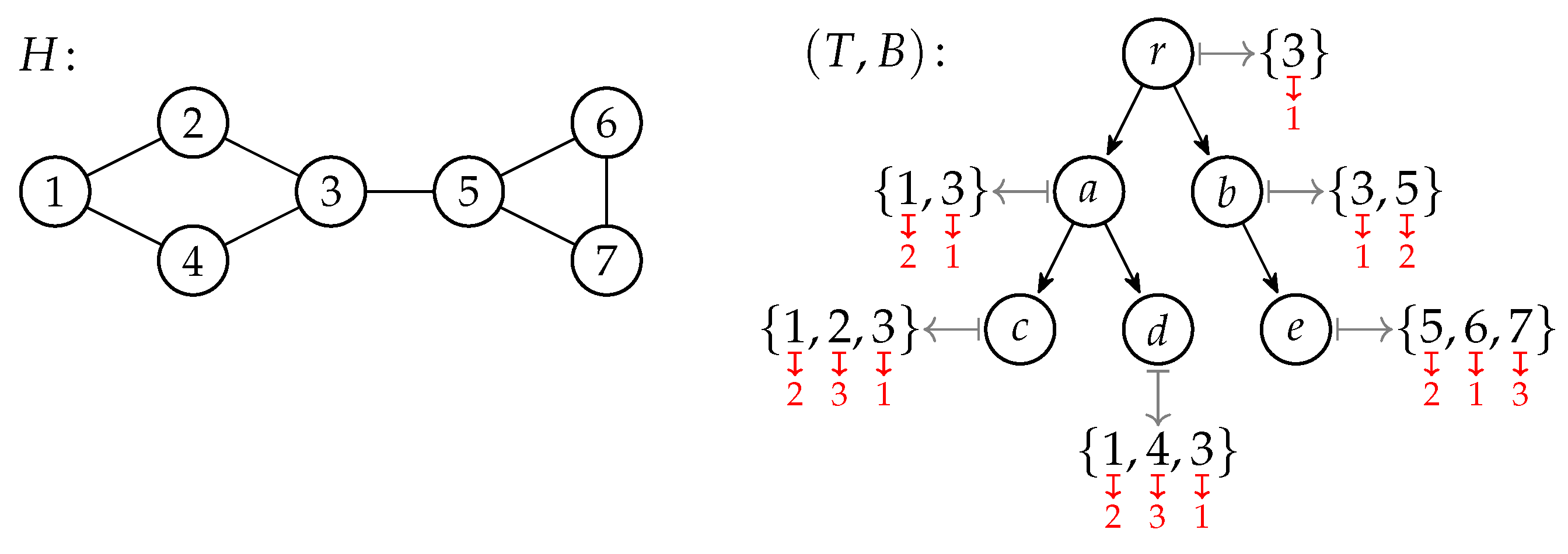
Table 1.
Membership of the problems discussed in this paper in the two classes and and the formulas whose syntactic structures prove this. Except for clique problem, formulas exist where at least the number of strong variables is independent of the parameter—but it is not always the most “natural” formulas that have this desirable property, see the vertex cover problem.
| Problem: Does a graph have a size-k matching? |
| Formulas: , see Equation (1) |
| Descriptive complexity: , |
| Problem: Does a graph contain k vertex-disjoint triangles? |
| Formulas: ( |
| , see Equation (2) |
| Descriptive complexity: , |
| for a fixed graph (instead of triangles) |
| Problem: Does a graph contain k vertex-disjoint induced copies of H? |
| Formulas: ( |
| Descriptive complexity: , |
| Problem: Does a graph contain a path of length k? |
| Formulas: |
| Descriptive complexity: , , see Equation (5) |
| Problem: Does a graph have a size-k vertex cover? |
| Formulas 1: |
| Descriptive complexity: , |
| Formulas 2: Describe the Buss kernelization, see Theorem 5 |
| Descriptive complexity: , |
| Problem: Does a hypergraph with maximum edge size d a size-k hitting set? |
| Formulas: Describe a kernel based on pseudo-sunflowers, see Theorem 6 |
| Descriptive complexity: , |
| Problem: Is a model of a graph with maximum degree ? |
| Formulas: Describe the disjointness of balls in the formula resulting from Gaifman’s Theorem using weak variables, see Theorem 7 |
| Descriptive complexity: , |
| and |
| Problem: Can H, of tree depth or width c, be embedded into a graph G? |
| Formulas: Bind the vertices of H’s image to weak variables and use a formula whose syntactic structure exactly mimics an optimal tree decomposition of H, see Theorem 8 |
| Descriptive complexity: , |
| Problem: Does a graph contain a k-clique? |
| Formulas 1: , see Equation (3) |
| Formulas 2: , see Equation (19) |
| Descriptive complexity: , in both cases |
Publisher’s Note: MDPI stays neutral with regard to jurisdictional claims in published maps and institutional affiliations. |
© 2021 by the authors. Licensee MDPI, Basel, Switzerland. This article is an open access article distributed under the terms and conditions of the Creative Commons Attribution (CC BY) license (http://creativecommons.org/licenses/by/4.0/).
Share and Cite
MDPI and ACS Style
Bannach, M.; Tantau, T. On the Descriptive Complexity of Color Coding. Algorithms 2021, 14, 96. https://0-doi-org.brum.beds.ac.uk/10.3390/a14030096
AMA Style
Bannach M, Tantau T. On the Descriptive Complexity of Color Coding. Algorithms. 2021; 14(3):96. https://0-doi-org.brum.beds.ac.uk/10.3390/a14030096
Chicago/Turabian StyleBannach, Max, and Till Tantau. 2021. "On the Descriptive Complexity of Color Coding" Algorithms 14, no. 3: 96. https://0-doi-org.brum.beds.ac.uk/10.3390/a14030096
Note that from the first issue of 2016, this journal uses article numbers instead of page numbers. See further details here.