
Lexicographic Unranking of Combinations Revisited


CNRS, Laboratoire de Paris 6—lip6—umr 7606, Sorbonne Université, F-75005 Paris, France
*
Author to whom correspondence should be addressed.
Algorithms 2021, 14(3), 97; https://0-doi-org.brum.beds.ac.uk/10.3390/a14030097
Submission received: 30 November 2020
/
Revised: 15 March 2021
/
Accepted: 16 March 2021
/
Published: 19 March 2021
(This article belongs to the Special Issue Selected Algorithmic Papers From CSR 2020)
Abstract
:In the context of combinatorial sampling, the so-called “unranking method” can be seen as a link between a total order over the objects and an effective way to construct an object of given rank. The most classical order used in this context is the lexicographic order, which corresponds to the familiar word ordering in the dictionary. In this article, we propose a comparative study of four algorithms dedicated to the lexicographic unranking of combinations, including three algorithms that were introduced decades ago. We start the paper with the introduction of our new algorithm using a new strategy of computations based on the classical factorial numeral system (or factoradics). Then, we present, in a high level, the three other algorithms. For each case, we analyze its time complexity on average, within a uniform framework, and describe its strengths and weaknesses. For about 20 years, such algorithms have been implemented using big integer arithmetic rather than bounded integer arithmetic which makes the cost of computing some coefficients higher than previously stated. We propose improvements for all implementations, which take this fact into account, and we give a detailed complexity analysis, which is validated by an experimental analysis. Finally, we show that, even if the algorithms are based on different strategies, all are doing very similar computations. Lastly, we extend our approach to the unranking of other classical combinatorial objects such as families counted by multinomial coefficients and k-permutations.
1. Introduction
One of the most fundamental combinatorial objects is called a combination. A combination of k objects among n is a subset of cardinality k of a set containing n objects. In many enumerating problems, it appears either as the main combinatorial structure or as a core building block because of its simplicity and counting characteristics.
In the 1960s while resolving some optimization problems related to scheduling, Lehmer rediscovered an important property linking natural numbers with a mixed radius numeral system based on combinations. This relation gave him the possibility to exhibit some greedy approach for a ranking algorithm that transforms (bijectively) a combination into an integer. This numeral system is now commonly called the “combinatorial number system” or “combinadics”. It is often used for the reverse of Lehmer’s problem: generating the uth combination (for a given order on the set of combinations). For efficiency reasons, this approach can be substituted to exhaustive generation once the latter is no longer possible due to the combinatorial explosion of the number of objects when their size increases. In the context of combinations, the explosion appears quickly (we recall that ). This generation strategy of a single element is classically called an unranking method. It appears as the fundamental problem in combinatorial generation such as in [1] and in optimization [2]. It is also used as a basic building block in scheduling problems [3], as well as, e.g., in software testing [4]. In other contexts, it appears as the core problem for the generation of complex structures: we can for example cite phylogenetics [5] and bioinformatics [6].
Prior to speaking of unranking one must specify a total order over the objects under consideration. The one that is frequently used is the lexicographic order; since it is humanly easy to handle, it has been extensively studied. However, as Ruskey mentioned [7] (p. 59), lexicographic generation is usually not the most efficient, thus particular care must be taken while unranking for this order. Knuth dedicated a section to the lexicographic generation of combinatorial objects, especially combination [8], relating it to the special case of Gray codes. Usually, while describing an unranking method, the dual approach for ranking, i.e., taking a built object and computing its rank, is also studied. The above reference to Knuth presents such algorithms. Other combinatorial objects are also studied in Ruskey’s book about combinatorial generation [7] and in Skiena’s book dedicated to the practical implementation of such algorithms [9]. For another ad hoc approach focused on the efficiency aspects of the ranking problem, one can refer to the work of Ryabko [10].
The classical approach for the construction of combinatorial structures presenting a recursive decomposition schema consists in taking advantage of this decomposition in order to build a bigger object from smaller ones. The method is detailed in the famous book by Nijenhuis and Wilf [11]. There, the authors were mostly interested in exhaustive generation and uniform random sampling, but some ideas about the decomposition schema are also applicable in the unranking context. The method has been applied generically to decomposable objects in the sense of analytic combinatorics, first in the context of recursive generation [12], and then in the context of unranking approaches [13].
Aside from such generic approaches there exist several ad hoc algorithms. The paper by Kokosinski [14] presents a comparative study of several of them. The complexity analysis of these algorithms have been settled to be linear in n on average over all possible combinations when k is ranging from 0 to n.
However, to the best of our knowledge, these complexity analyses are only counting the number of calls to the function that computes a binomial coefficient, assuming that all the necessary coefficients have been pre-computed and stored (this pre-computation step is not included in the complexity analysis). From this fact, two questions arise. First, is this complexity analysis relevant? That is, does it faithfully reflect the actual runtime of the algorithms and can we afford the pre-computation of that many binomial coefficients? Second, among the different existing algorithms, which one performs best in practice?
Using exact computations, it is actually not a problem to deal with combinations over sets of several thousands of objects. In this context, using a table filled with all possible binomial coefficients that might be needed is impractical. Most classical computer algebra systems (CAS) can unrank combinations in a reasonable time though, which suggests that there are better approaches. In Table 1, we present some of our experimental results. We detail everything in Section 4, but as a foretaste here we give some key points. In Section 2, we introduce a new unranking algorithm. The first column gives the typical run time of our C implementation of this algorithm. In the other columns, we give a rough performance comparison of four different CAS. For each one, we compare the average run time in milliseconds to unrank a combination first by using the native algorithm of the CAS (“their algo.”) and second by implementing our new algorithm in the high-level programming language of the CAS. We observe a great diversity of run times in Table 1. Unfortunately, Maple, Mathematica, and MATLAB (to deal with integers with arbitrary precision in MATLAB, we use symbolic computations by calling the function sym) are all closed source so we cannot take a look at their implementation to understand these differences. However, a detailed study of the different algorithms from the literature and some practical considerations presented in Section 4 provide some insights on this question. Sagemath is a special case to us. Since version 9.1, our algorithm has been implemented (in Python 3) and is used as the native algorithm.
Combinatorial Context
Throughout the paper, we represent combinations as follows.
Definition 1.
Let n and k be two integers with . We represent a combination of k elements among n elements denoted by as a finite increasingly sorted sequence containing k distinct elements.
For example, let n and k be, respectively, 5 and 3. The finite sequences and are combinations of k elements among n, but and are not. Other representations are sometimes used, notably by using a two-letter alphabet, but we stick to the one given in Definition 1 in this paper.
There are several possible orders for comparing combinations. In the following, we restrict our attention to orders comparing combinations of the same length, i.e., the same number of elements.
Definition 2.
Let and be two distinct combinations of k elements among n.
- In the lexicographic order, we say that A is smaller than B if and only if both combinations have the same (possibly empty) prefix such that and if in addition .
- In the co-lexicographic order, we say that A is smaller than B if and only if the finite sequence is smaller than for the lexicographic order.
- If A is smaller than B for a given order, then, for the reverse order, B is smaller that A.
Definition 3.
Let be two integers and let A be a combination of k elements among n. For a given order, the rank u of A belongs to and is such that A is the uth smallest combination.
With these definitions in mind, we can enter the core of the paper organized as follows. We first give the presentation and a first complexity analysis of our new algorithm solving the lexicographic combination unranking problem in Section 2. Section 3 is dedicated to the survey of three classical algorithms for the latter problem. The first one is based on the so-called recursive method and the two other algorithms are based on combinadics, which is a specific numeral system. It seems that it is the first time that both are compared and the reason one is better is explained. We also propose a new method for their analysis based on a generating function approach. Obviously, we obtain the same results as in the literature, but we manage also to obtain better asymptotic bounds than in the literature. In Section 4, we then compare their efficiency experimentally (the implementation and the exhaustive material used for repeating the experiments are all available at http://github.com/Kerl13/combination_unranking (accessed on 15 March 2021)) and propose a way to improve the computation of the binomial coefficients used in all four algorithms. Surprisingly, once the improvements have been implemented in all algorithms, we observe deep similarities in their computations, which is reflected by their observed run times. Finally, we extend our approach to solve the problem of unranking structures enumerated by multinomial coefficients and also objects counted by the k-permutations of n (also called arrangements).
2. Unranking through Factoradics: A New Strategy
The classical methods to unrank combinations are relying on the combinatorial number system introduced in 1887, by E. Pascal [15] and later by D. H. Lehmer (detailed in the book [16] (p. 27)). We survey these classical algorithms in Section 3.2. In this section, we first present a new strategy based on another number system called factoradics. To the best of our knowledge, the latter has never been used for the unranking of combinations.
2.1. Link between the Factorial Number System and Permutations
We recall that the factorial number system, or factoradics, is a mixed radix numeral system in which the representation of integers relies on the use of factorial numbers. Its definition belongs to the folklore but already appeared in 1888 in [17].
Definition 4.
Let u be a positive integer and let n be the unique integer satisfying . Then, there exists a unique sequence of integers , with for all ℓ, such that:
The finite sequence is called the factoradic decomposition (or factoradic) of u (note that for all u).
Taking the number u = 2021 as an example, we obtain the following decomposition: 2021 = . Thus, its factoradic is .
Definition 5.
Let n be a positive integer. A permutation of size n is an ordering of the elements of the set .
We represent a permutation of size n as a finite sequence of length n indicating the order of its elements. For example, the sequence is a permutation of size 5.
The factorial number system is particularly suitable to define a one-to-one correspondence between integers and permutations and thus can be used as an unranking method for permutations. The algorithm implemented in the function UnrankingPermutation in Algorithm 1 is a straightforward adaptation of the Fisher–Yates random sampler for permutations [18].
Fact 1.
For all ,UnrankingPermutation returns the uth permutation in lexicographic order among the permutations of n elements.
| Algorithm 1 Unranking a permutation. | ||
| 1: function Extract(F,n,k) | ||
| 1: function UnrankingPermutation(n,u) | 2: P ← [0,1,…,n − 1] | |
| 2: F ← factoradic(u) | 3: L ← [0,…,0] | ▷ k components |
| 3. while do | 4. for i from 0 to do | |
| 4: | 5: | |
| 5: return | 6: | |
| 7: return L | ||
| factoradic: computes the factoradic of u; | ||
| length: computes the number of components in F; | ||
| append: appends the element i at the end of F; | ||
| remove: removes from F the element at index i. | ||
Since the factoradic (with 8 components) of 2021 is , the permutation (of size 8) of rank 2021 is . To obtain this permutation, we read the factoradic from right to left, and extract iteratively from the list the element whose index is the coefficient read in the factoradic. This goes on until the list is empty and we reach the leftmost component of the factoradic. Thus, in our example, we start by extracting the element of index 0, which is 0. Then, the list P becomes and we extract the element of index 2, which is 3. Then, P becomes and we extract the fourth element, which is 6, and so on.
Note that, for the sake of clarity, we present the function Extract using a list for P, but a better data structure must be used to achieve good performance. Good candidates are dynamic balanced trees, as presented in [19], or multisets with elements of weight 1 or 0, as presented in the Appendix of [20], since both provide logarithmic access and removal. Unfortunately, it seems that there is no algorithm based on some swap operation giving an in-place shuffle to unrank permutations in the lexicographic order; put differently: Durstenfeld’s algorithm [21] cannot be easily adapted for the lexicographic order.
2.2. Combinations Unranking through Factoradics
We start with the definition of our algorithm to unrank combinations via the use of factoradics. The basic ideas driving our algorithm are the following:
- We define a bijection between the combinations of k elements among n and a subset of the permutations of n elements.
- We transform the combination rank u into the rank of the appropriate permutation.
- We build (the prefix of) the permutation of rank by using Algorithm 1.
Definition 6.
Let n and k be two integers with . We define as the function which maps the combination to the size-n permutation where the integers are such that and .
For instance, by definition, for and , the permutations associated with the combinations and are, respectively, and . Note that the function returns the smallest size-n permutation for the lexicographic order whose prefix is the given combination.
Proposition 1.
For all integers , the function is a bijection from the set of combinations to the set of size-n permutations whose prefix of length k and suffix of length are both increasingly sorted.
Remark that the permutation (of size 5) is the permutation associated with combinations and by, respectively, and . In fact, there are exactly six combinations associated with the latter permutation, but for different values of k. The proof of Proposition 1 is straightforward.
Fact 2.
For any integer , the number of sequences satisfying is given by .
In fact, we get this result using a classical cardinality argument: a sequence of integers of the form corresponds to a weak composition (consider the differences ) of the integer ℓ into terms. The number of such compositions is given by . Hence, the number of sequences matching the description of Fact 2 is given by .
We now exhibit how to transform a combination rank into its corresponding permutation rank.
Lemma 1.
For any given , the factoradic decompositions of the ranks of the permutations obtained as the image by of some combination of k elements among n are all the finite sequences of the form with .
Proof.
Let u be an integer whose factoradic is as in the lemma. Due to the constraint , the permutation corresponding to u has for prefix of length k the sequence which is increasingly sorted. The rest of the permutation (the suffix of length ) corresponds to the increasing sequence of elements that have not been taken yet. Thus, the result corresponds to a combination via .
Fact 2 completes the proof. □
Thus, to convert the combination rank u into its corresponding permutation rank , it is sufficient to find the uth sequence satisfying Lemma 1 in co-lexicographic order. This is presented in Algorithm 2 where the RankConversion function implements the conversion from u to and the UnrankingCombination function implements the whole unranking procedure.
The key to the rank conversion is also Fact 2. As a consequence, we get that the first such sequences (in co-lexicographic order) have and that the following have .
Once again, we opt for a simple presentation here where the rank conversion and the unranking part of the algorithm are clearly separated. There is much room for improvement here: for instance, note that, at the end of the function RankConversion, a factoradic decomposition is transformed into the integer it represents, but then at the beginning of UnrankingPermutation this integer will be decomposed again in factoradics. In fact, instead of storing m into F on Line 8 we could directly compute the ith component of the combination as by using the remark at the beginning of the proof of Lemma 1. In Section 4.2, we provide a more efficient way to implement this algorithm including this particular optimization and other improvements.
Proposition 2.
The functionUnrankingCombination computes the uth combination of k elements among n in lexicographic order.
Proof.
The algorithm, and thus its proof, relies heavily on Fact 2. The key to prove the correctness of the RankConversion function is the following loop invariant:
- The values of for all have been computed and stored in F.
- The value of (which has not been determined yet, as we enter the loop) is at least m.
- The variable holds the rank of the sequence (note that ) among all sequences satisfying the condition of Fact 2 with and .
With this invariant at hand, the combinatorial argument behind the condition in the algorithm becomes more apparent; that is, the binomial coefficient counts the number of such sequences ending with m. Hence, if , then and we move to the evaluation of the next coefficient (); otherwise, we try the next possible value for m. □
| Algorithm 2 Unranking a combination. | ||
| 1: function RankConversion(n,k,u) | ||
| 2: F ← [0,…,0] ▷ n components in F | ||
| 3: i ← 0 | ||
| 4: m ← 0 | ||
| 5: while i < k do | ||
| 1: function UnrankingCombination(n,k,u) 2: u′ ← RankConversion(n,k,u) 3: p ← UnrankingPermutation(n,u′) 4: return the first k elements of p | 6: b ← binomial(n − 1 − m − i,k − 1 − i) | |
| 7: if b > u then | ||
| 8: F[n − 1 − i] ← m | ||
| 9: i ← i + 1 | ||
| 10: else | ||
| 11: u ← u − b | ||
| 12: m ← m + 1 | ||
| 13: ▷F is the factoradic decomposition | ||
| 14: return composition(F) | ||
| binomial(n,k) computes the value of ; | ||
| composition(F): computes the integer whose factoradic is F. | ||
The usual way to evaluate the efficiency of such an algorithm is to count the number of times the binomial function is called (see, e.g., the book [7] (p. 66) or the papers [22,23]). During the conversion from the rank of the combination to the one of the associated permutation, the coefficients are obtained via trials (in the factoradic notation) for to , remarking that through our bijection the latter sequence is weakly increasing. Thus, the worst cases are obtained when the value is as large as possible, that is . In these cases, the number of calls to binomial is n.
To study the average number of calls to binomial, when u describes the whole range from 0 to , we introduce the following cumulative sequence.
Lemma 2.
Let be the cumulative numbers of calls to binomial while unranking all possible combinations u from 0 to . The sequence satisfies: and for all n and , and otherwise:
In Table 2, we give the first values of , when n is less than 9. The obtained sequence is stored under the reference OEIS A127717 (throughout this paper, a reference OEIS A⋯ points to Sloane’s Online Encyclopedia of Integer Sequences www.oeis.org (accessed on 15 March 2021)). The bijection between both structures is direct, and thus we provide new information about this sequence in the following.
Proof.
The recurrence can be observed by unrolling the first iteration of the while loop. In the first iteration of the loop, a binomial coefficient b is always computed (regardless the value of k and n) which accounts for the term in the recurrence relation. Then, for all the ranks u such that , we choose and increment i, so that the rest of the execution corresponds to unranking a combination of elements among . This is accounted for by . Conversely, for all ranks u such that , the value of m is incremented and the rest of the execution corresponds to unranking a combination of k elements among , which is accounted for by □
We turn to bivariate generating functions to encode the sequence as a power series and express the above recurrence as a simple equation satisfied by this function, which can be solved explicitly. The reader can refer to the two books of Flajolet and Sedgewick [24,25] for a global presentation of such method.
Theorem 3.
Let be the generating functions associated with . Then,
Proof.
The first step of the proof consists in exhibiting the ordinary generating function associated with . To obtain a functional equation satisfied by U, we start from the result presented in Lemma 2. The extreme cases are and for all n and . The recursive equation is .
We remark the constant in the equation. We thus need the bivariate generating function of binomial coefficients. Let us denote it by , which is equal to
To take into account the extreme cases, we must remove the terms corresponding to :
By summing both sides of the recursive relation and by taking care of the extreme cases, we get:
We thus deduce
The second step in the proof consists in extracting the coefficient . We rewrite as:
By extraction, the coefficient in front of is:
The latter result corresponds to the distribution of the costs when k varies from 0 to n. We can then exactly extract the coefficient of :
□
Corollary 1.
To unrank a combination of k elements among n, the function UnrankingCombination needs on average calls to the function binomial. For n being large and k being of the form for , this average number of calls is
The result is direct by using Theorem 3. Since we have the exact value of , the mean value can easily be computed in other cases such as or .
3. Classical Unranking Algorithms
This section is dedicated to the presentation of a survey of the usual approaches to unrank combinations in the lexicographic order. The motivation behind this section is threefold. First, the classical algorithms were developed in the 1970s and 1980s and it is a hard task to get access to the papers we mention. Second, although they have been analyzed according to the number of calls to the binomial coefficient computations, we present here a standardization of the analysis using generating functions such as in the previous section. Finally, as shown in Section 4 and in the conclusion of the paper, a detailed analysis of all the possible approaches is necessary to well understand the behaviors of the computations.
3.1. Unranking through the Recursive Method
We are dealing with a combinatorial structure here, combinations, that is well understood in the combinatorial sense. Thus, when trying to develop an unranking algorithm, the first idea consists in developing one based on the classical recursive generation method presented in [11]. This type of algorithm is based on a recursive decomposition of the structure into smaller parts. Here, this idea is to use the following fact: a combination of k elements among either contains or does not. In the first case, the rest of the combination can be seen as a combination of elements among and in the second case the combination is a combination of k elements among . From a counting point of view, this translates into the well-known identity and, from an unranking point of view, this translates into Algorithm 3.
| Algorithm 3 Recursive Unranking. | |
| 1: function UnrankingRecursive(n,k,u) 2: L ← RecGeneration(n,k,u) 3: L′ ← [0,…,0] ▷ k components 4: for i from 0 to k − 1 do 5: L′[i] ← n − 1 − L[k − 1 − i] 6: return L′ | 1: function RecGeneration(n,k,u) 2: if k = 0 then 3: return [] 4: if n = k then 5: return [0,1,2,…,k − 1] 6: b ← binomial(n − 1,k − 1) 7: if u < b then 8: R ← RecGeneration(n − 1,k − 1,u) 9: append(R,n − 1) 10: return R 11: else 12: return RecGeneration(n−1,k,u−b) |
Remark 1.
An alternative choice would have been to test whether on Line 6. This corresponds to putting first the combinations that do not contain and then those that contain . In this case, the unranking order is different but the performance is similar.
Proposition 3.
The functionRecGeneration(n,k,u) computes the uth combination of k elements among n for the reverse co-lexicographic order.
Corollary 2.
The functionUnrankingRecursive(n,k,u) computes the uth combinations of k elements among n for the lexicographic order.
Proof.
The proposition is proved by induction and the corollary is a direct observation given in [26] (p. 47). □
Here, again, we are interested in the average number of calls to the binomial function, when u describes the whole range of integers from 0 to . Ruskey justified such a measure by supposing the table of all binomial coefficients pre-computed, thus each call is equivalent. In Section 4, we discuss this measure. We introduce the sequence (to simplify the notations, we use several times the notations and for distinct sequences and series) equal to the cumulative number of calls to binomial for the whole range of possible values for u.
Lemma 3.
Let be the cumulative number of calls to binomial for the recursive unranking while unranking all possible u from 0 to . The sequence satisfies: and for all n and , and otherwise
Proof.
If , calling RecGeneration(n,k,u) incurs one call to binomial and a recursive call. The cumulative cost of the first call to binomial is , the cumulative cost of the recursive calls for is and the cumulative costs of the recursive calls for is . □
In the following Table 3, we give the first values of , when n is less than 9.
Theorem 4.
Let be the ordinary generating function associated with , such that . Then,
The proof of Theorem 4 is very similar to the one of Theorem 3.
Proof.
The first step of the proof consists in exhibiting the ordinary generating function associated with . To obtain the equation for U, we start from the result presented in Lemma 3. The extreme cases are and for all n and . The recursive equation is .
Again, the numbers appear in the equation, thus we need the bivariate generating function of binomial coefficients. Let us denote it by . It satisfies:
To follow the extreme cases, we must remove the first column and the diagonal :
By summing the recursive equation and taking care of the extreme cases, we get:
We thus deduce
The second step of the proof consists in extracting the coefficient .
By extraction the coefficient in front of is:
The latter result corresponds to the distribution of the costs when k varies from 0 to n. We can then extract the coefficient of :
which completes the proof. □
This sequence is a shifted version of the sequence stored under the reference OEIS A059797. We thus can complete its properties in the OEIS using our results.
Due to the values of the extreme cases when and and the symmetry in the recurrence, we obviously obtain that , reflecting the symmetry of the binomial coefficients.
Corollary 3.
The functionUnrankingRecursive(n,k,·) needs on averagecalls to the function binomial. For n being large and k being of the formfor, we get:
Note that, for this algorithm too, the average complexity is only below the worst-case complexity by a constant (when ).
Naturally, to be able to handle large values of n and k, a tail-recursive variant of this algorithm, or an iterative version, should be preferred over the straightforward implementation. The recursive approach is a drawback for some programming languages that do not handle recursion efficiently (due to the depth of the stack). Naturally, other strategies have been suggested in the literature.
3.2. Unranking through Combinadics
In 1887, E. Pascal [15] and later D. H. Lehmer (detailed in the book [16] (p. 27)) presented an interesting way to decompose a natural number, in what we call today a mixed radix numeral system. In their case, it is the so-called combinatorial number system, or combinadics. The decomposition relies on binomial coefficients.
Fact 5.
Let be two positive integers. For all integers u, with , there exists a unique sequence such that (we extend the definition of binomial coefficients with when )
The finite sequence is called the combinadic of u.
For example, when and , the number 8 is represented as , thus the combinadic of 8 is . In Table 4, we present for various values of u the combinadic of u and the combination of rank u for and . Here, we observe that the exhibited ranking is co-lexicographic and that the combination of rank u can be deduced from the combinadic of u by reversing it and applying the transformation to each of its components.
In 2004, using this representation, McCaffrey exhibited, in the MSDN article [27], an algorithm to build the uth element (in lexicographic order) of the combinations of k elements among n. However, in fact, this algorithm was already published by Kreher and Stinson [26] (p. 47) and can also be seen as an extension of the work of Lehmer. This algorithm is interesting as it corresponds to the previous implementation used in the mathematics software system Sagemath [28] (the previous unranking algorithm from Sagemath is stored in the Software Heritage Archive swh:1:cnt:c60366bc03936eede6509b23307321faf1035e23;lines=539-605). In the beginning of 2020, we replaced the Sagemath implementation by the algorithm presented in Section 2 (the new unranking algorithm from Sagemath is stored in the Software Heritage Archive swh:1:cnt:b2a68056554dbf90fa55e76820f348d9d55019e3;lines=539-653 (accessed on 15 March 2021)).
The algorithm simply performs the combinadic decomposition of u and then applies the aforementioned transformation. The idea to get the combinadic of an integer is the following: is obtained as the maximum integer such that , and then the remaining part is smaller than so it can be decomposed recursively into a combinadic with components smaller than . McCaffrey’s algorithm is described in Algorithm 4.
| Algorithm 4 Unranking a combination. |
| 1: function UnrankingViaCombinadic() |
| 2. ▹k components |
| 3. |
| 4. |
| 5. for i from 0 to do |
| 6. |
| 7. |
| 8. while do |
| 9. |
| 10. |
| 11. |
| 12. |
| 13. return L |
As noted while explaining Table 4, we work with the reverse of the rank u (see Line 3 in the algorithm) in order to unrank combinations in lexicographic order. The presented algorithm is also close to Er’s algorithm [23] whose representation for combinations is distinct, but the computations are analogous; furthermore, in his paper, Theorem 2 corresponds exactly to the combinadic decomposition.
The function computes the combinations of k elements among n of rank u in lexicographic order, although the core of the algorithm is reverse co-lexicographic. The correctness of the algorithm is stated in [26].
Again, we express the complexity of this algorithm as its number of calls to the binomial function. First note that, the values n and k being given, the worst cases are obtained when v gets as small as possible at the end of the loop, thus for all u whose combinadic satisfies . Hence, the worst case complexity is . Again, we complete this analysis, by computing the average complexity of the algorithm. To reach this goal, we again introduce the sequence computing the cumulative number of calls to binomial when u ranges from 0 to .
Lemma 4.
Let be the cumulative numbers of calls to binomial while unranking all possible u from 0 to . The sequence satisfies: and for all n and , and otherwise
Table 5 presents the sequence given in Lemma 4. The difference with the two sequences studied before lies in the extreme cases. This sequence is a shifted version of the sequence OEIS A264751. Both combinatorial objects can be put in bijection, and thus some conjectures stated there are solved in the following.
Proof.
Note that calls to binomial are necessary to determine , then calls to determine , …, and finally to determine . Hence, the total number of binomial coefficients evaluations necessary to compute the combinadic of u is (and thus only depends on ). Besides, for a given , the number of finite sequences is equal to the number of sequences by the change of variable . Hence, this number is equal to . In addition, there is a first call to binomial at the beginning of the algorithm to reverse the rank, regardless of the value of u. We thus obtain:
Using the latter equation, the recursive equation is directly proved by induction. □
Note that in this case the cumulative numbers are not symmetrical . In fact, the computation of the combinadics is not symmetrical.
Theorem 6.
Let be the generating function associated with . Then,
The proof is the same as for Theorem 3. The values for are a bit different due to the extreme cases .
Corollary 4.
The average number of calls to binomial in Algorithm 4 for n being large and k being of the form for is
In the literature, another algorithm based on combinadics is given in [22]. We provide a pseudo-code equivalent of the original Fortran algorithm in Algorithm 5. Note that the algorithm does not handle the case , which should thus be treated separately. There, in the computation of the combinadic for a given rank, the coefficients are computed from the smallest one, , to the second largest one, , and finally the value for is directly deduced with no need for further trials. In this algorithm, the variable L contains the combinadic of u (not its reverse). We note two differences with Algorithm 4. First, the last coefficient () is directly computed without “trying” the different possible values as for the previous coefficients (see Line 13 ). Second, it uses a combinatorial argument to find the value of the coefficients that is the complementary of the argument used in the previous algorithm: the number of sequences with is equal to , hence the accumulation performed in the r variable. The fact that the same combinatorial argument can be used in two different ways here has to be put in parallel with Remark 1 at the beginning of this section.
The first point mentioned above is an improvement over Algorithm 4, but in fact this second algorithm is penalized by the extra addition that it has to perform and then undo on Line 12 to find each . With this approach, it is mandatory to compute the accumulation of binomial coefficients in r until it becomes greater than u to know when to exit the loop. It appears in our experimentations in the next section that this has a noticeable impact on performance.
| Algorithm 5 Unranking a combination (alternative algorithm). |
| 1: function UnrankingViaCombinadic2() |
| 2: ▹k components |
| 3. |
| 4. for i from 0 to do |
| 5. if then |
| 6: else |
| 7: while true do |
| 8: |
| 9: |
| 10: |
| 11: if then exit the loop |
| 12: |
| 13: |
| 14: return L |
UnrankingViaCombinadic2(n,k,u) is a lexicographic unranking for combinations. This algorithm was presented by Buckles and Lybanon [22], and its correctness is presented in [26]. Finally, note it is approximately the implementation in Matlab [29] whose code was also presented by Ruskey ([7], p. 65). The latter approach also does trials to find the last coefficient of the combination instead of computing it directly on Line 13.
Lemma 5.
Let be the cumulative numbers of calls to binomial while unranking all possible u from 0 to . For all n, the sequence satisfies when or , and otherwise
The result is proved in an analogous way as Lemma 4, summing over instead of . In Table 6, we compute the first values of . We note the first values are smaller than the previous ones, and Theorem 7 gives their asymptotic behavior.
Theorem 7.
Let be the generating functions associated with . Then,
Corollary 5.
The average number of calls to binomial in Algorithm 5 for n being large and k being of the form for is
The improvement for the efficiency of the algorithm is seen only on the second order in comparison to the one of Corollary 4 on average. Let us conclude this part with an interesting remark.
Remark 2.
In our Algorithm 3, while unranking k elements among n, we combinatorially see as first and otherwise at . This is the same approach as in Algorithm 5. However, as explained after Algorithm 3, we could have first been interested in and then in . Then, the algorithm would have been in a reverse co-lexicographic fashion, and it would follow exactly the same approach as Algorithm 4.
4. Improving Efficiency and Realistic Complexity Analysis
Finally, we show that the complexity model used above is no longer adequate. Although the approximation that computing one binomial coefficient has a constant cost seems to have been sufficient in the past (due the limitation of the implementations to 32-bit integers; see the work of McCaffrey [27], who seems to be the first to introduce combination unranking using big integer computations), this is no longer a valid model as big integers are now more widely used. We discuss the impact of big integer arithmetic and some optimizations that significantly improve the performance of all algorithms.
From the two last sections, we know the different algorithms that are mostly used in practice. However, having in mind the results exhibited in Table 1, implementations may vary a lot. Obviously, using a specialized library for big integer arithmetic such as the GMP C library is the best way to carry out fast operations, but the distinct behaviors observed in the table suggests that deeper differences exists between the various implementations than just the choice of the library.
For all algorithms, we prove that the average number of calls to the binomial function is equivalent to n (when k grows linearly). A first question to investigate is about this complexity measure: Is it reasonable? An obvious approach consists in comparing these results with the actual run time of the algorithms.
4.1. First Experiments to Visualize the Time Complexity in a Real Context
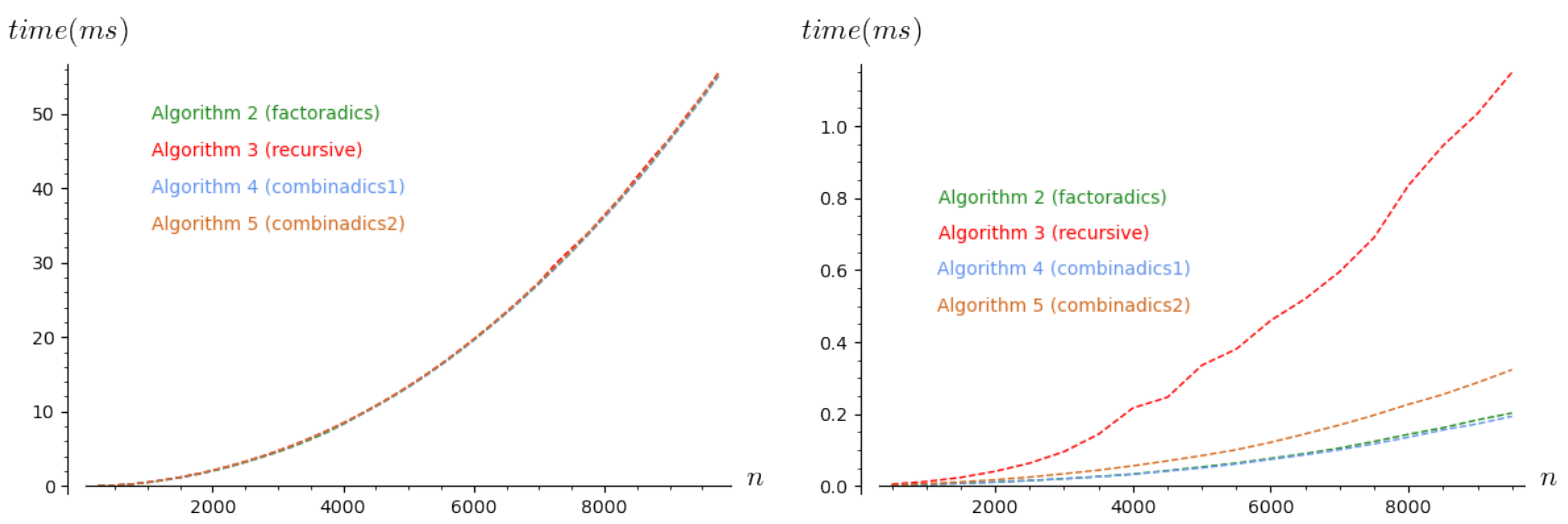
In the two next plots in Figure 1, we present the average time needed for the computations of 500 combinations for each pair where n ranges from 250 to 10,000 with a step size of 250. The choice was made because it corresponds to the worst complexity cases when k varies from 0 to n. To conduct our experiments, we implemented all algorithms in C using the classical GMP library for big integers arithmetic (the implementation and the exhaustive material used for repeating the experiments are available at http://github.com/Kerl13/combination_unranking (accessed on 15 March 2021)). The experiments were run on a standard laptop PC with an I7-8665U CPU, 32Gb RAM running Ubuntu Linux 2020. Moreover, except for Table 1, which required running different computer algebra systems and thus the X server, the experiments were run in the console while the X server and other time-consuming services (wifi, sound, etc.) were off. On the leftmost plot, we present the average time for the unranking of a combination for n ranging from 250 to 10,000 by steps of 250 too. Note that all the curves are merged: all algorithms seem to need almost exactly the same time to unrank a combination. In the rightmost plot, we present a version with memoization (memoization is an optimization technique consisting in storing the results of expensive function calls and returning the cached values when the function is called again with the same arguments; this technique is sometimes called “tabling”) for the algorithms: we first run a pre-computation step storing all binomial coefficients that will be used. The second step consists in unranking the combinations by using the pre-calculated values for the binomial coefficients. In our plot, we present only the time used for the second step. We remark that the recursive Algorithm 3 is not as efficient as the others. Below, we show that this is due to its recursive nature and that this can be easily avoided. As explained above, Algorithm 5 should be less efficient than Algorithm 4, which is indeed apparent in the plots. Our Algorithms 2 and 4 are the most efficient when used in this setup.
While the number of evaluations of binomial coefficients is linear in n, it is clear that it is not the case for the time complexity of the algorithms (see the leftmost plot). However, once the binomial coefficients have been pre-computed, running the four algorithms without computing binomial coefficients is closer to a linear function but they still are not really linear.
While memoizing all binomial coefficients when n is of order of some hundreds is possible, it is no longer the case when n is of the order of several thousands (for the experiments in Figure 1, we only computed the necessary binomial coefficients using a lazy approach). Such use cases did not occur when the methods (e.g., [22,23]) were derived. However, now that big integers are more widely used, it becomes reasonable to unrank combinations of large size and it is thus necessary to take the cost of arithmetic operations into account. The first use of big integers for combination unranking appears to date back to 2004 [27].
4.2. Improving the Implementations of the Algorithms
Before going further with the experiments, we propose an improvement in the computation of the binomial coefficient, which is applicable to all algorithms presented in this paper.
In all of the presented algorithms, a binomial coefficient is computed at each step of the generation. There are various ways to implement those. One possibility is to compute the two products and separately using a divide and conquer strategy as described in [30] (Section 15.3) and then to compute the division.
In the unranking algorithms, instead of doing the “full” evaluation of the binomial coefficient at each step, it is possible to reuse the computations from the previous step and obtain the value of the new coefficient by a constant number of multiplications or divisions by a small integer. This is possible because in all algorithms the parameters of the binomial coefficients vary only by from one step to the next. For instance, in Algorithm 2, just before incrementing i on Line 9, the coefficient for the next iteration can be obtained by multiplying b by and dividing it by . Similarly, in the other branch of the if, just before incrementing m on Line 12, the value of the coefficient for the next iteration can be obtained by multiplying b by and dividing it by . In the end, only the first binomial coefficient is computed from scratch and all others are obtained as described above. This lowers the amortized cost of computing one coefficient to multiplication of a big integer by a small integer. This optimization is applicable to all the algorithms presented in this paper.
In Algorithm 6, we propose an optimized version of our Algorithm 2 based on the above remarks. It also includes some other enhancements. First, instead of computing the permutation rank of the combination and then unranking the combination as a permutation, it is possible to process the coefficients of the factoradic decomposition on the fly to extract the right value from the set . Second, we can note that we are in a special use-case of the Extract function where values are extracted in increasing order. Hence, there is no need to explicitly store the set of remaining values (not yet in the combination) to get access to its mth value: it is where i is the number of already extracted values. Finally, the last component of the combination can be deduced without computing more binomial coefficients (Line 15) in order to leave the loop earlier.
Before going on with the efficiency comparisons, we use the remarks related to the binomial coefficient computation to improve Algorithms 3–5. Furthermore, to make the comparison fair, we used a variant of Algorithm 3 for the recursive approach in which the array storing the result is allocated with the right size at the beginning of the execution, as in the other algorithms. In addition, in order not to penalize it due to its recursive nature, the order of some instructions have been changed so that it is tail-recursive. The optimized version is given in Algorithm 7.
In UnrankTR, the variable i represents the position in L of the next value to be computed and the variable m represents the next candidate to be the value of . The invariant satisfied by b is that UnrankTR is always called with .
| Algorithm 6 Unranking a combination with optimization. |
| 1: function OptimizedUnrankingCombination() |
| 2: ▹k components |
| 3: |
| 4: ; |
| 5: while do ▹ Invariant: |
| 6: |
| 7: if then |
| 8: |
| 9: |
| 10: |
| 11: else |
| 12: |
| 13: |
| 14: |
| 15: if then |
| 16: return L |
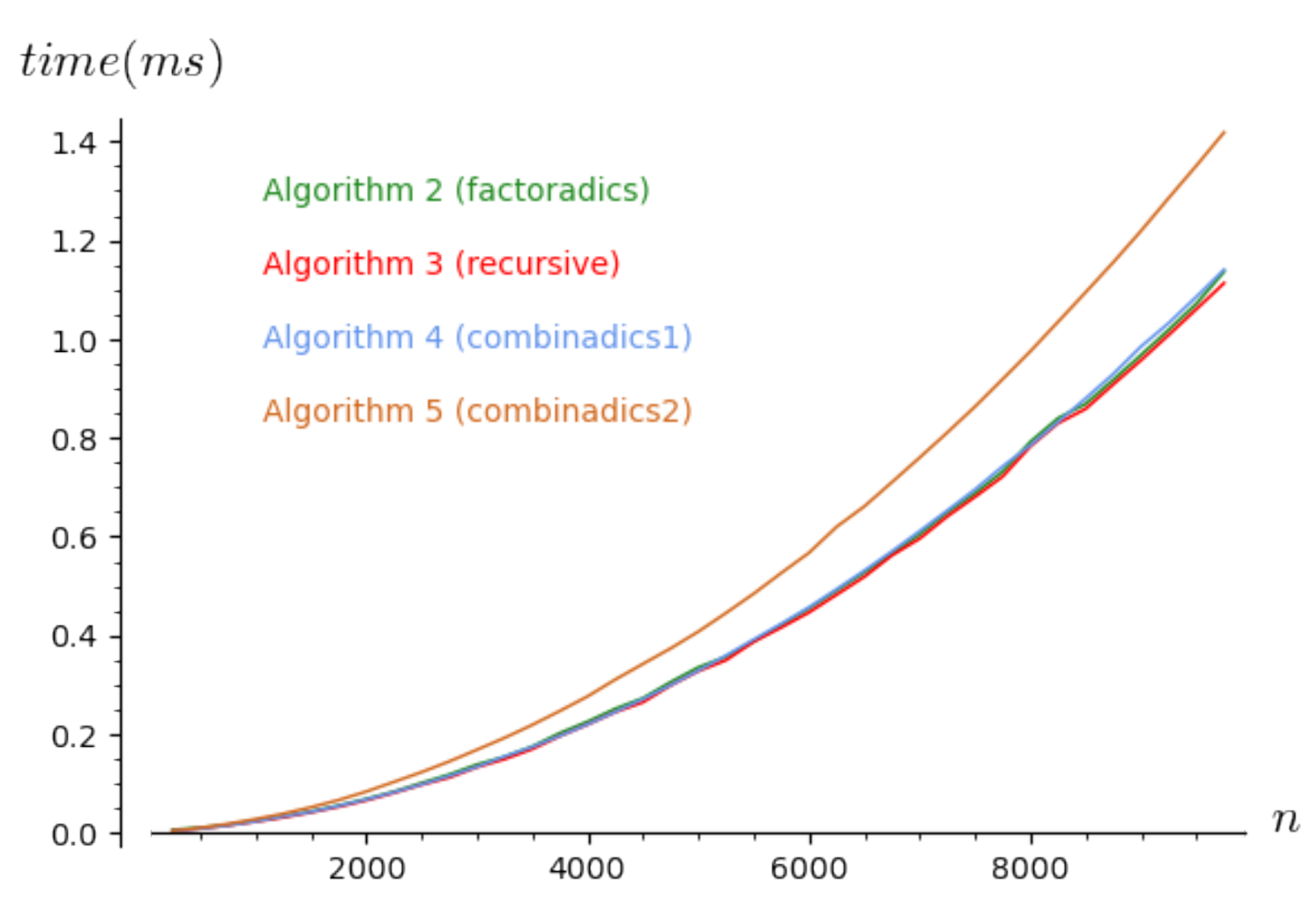
We propose a second time efficiency comparison for some algorithms with their optimizations in Figure 2. Comparing this plot with the leftmost one of Figure 1, we note that, when , the algorithms run approximately 45 times faster. Again, we note that Algorithm 5 is still less efficient than the others, which all seem to be equivalent.
| Algorithm 7 Recursive method with optimizations. | |
| 1: function OptimizedUnranking- Recursive(n,k,u) 2: L ← [0,…,0] ▷ k components 3: b ← binomial(n,k) 4: UnrankTR(L,0,0,n,k,u,b) 5: return L | 1: function UnrankTR(L,i,m,n,k,u,b) 2: if k = 0 then do nothing 3: else if k = n then 4: for j from 0 to k − 1 do 5: L[i + j] ← m + j 6: else 7: b ← b/n 8: if u < b then 9: L[i] ← m 10: b ← (k − 1) · b 11: UnrankTR(L,i + 1,m + 1,n − 1,k − 1,u,b) 12: else 13: u ← u − b 14: b ← (n − k) · b 15: UnrankTR(L,i,m + 1,n − 1,k,u,b) |
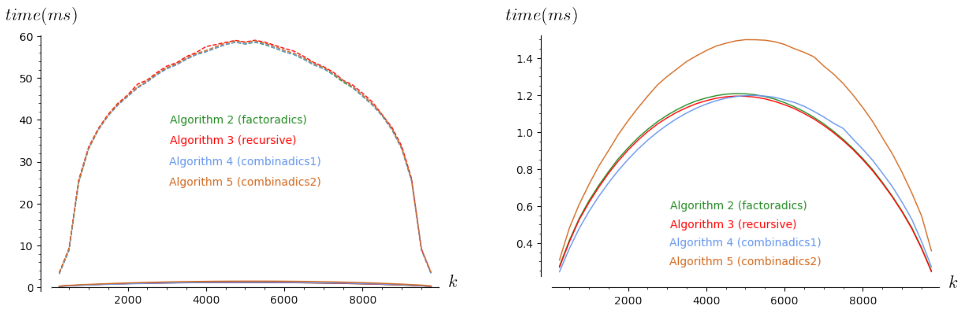
To understand the behavior of the curves of the above plot, we introduce another way to analyze the time complexity in Figure 3. Now, we take and we let k range from 250 to with an iteration step of 250. For each step, we present an average value for 500 tests. Again (in the leftmost plot), the dashed lines correspond to the first version of each algorithm and the solid lines to the optimized versions. In the rightmost plot, we only focus on the optimized versions of the four algorithms. We remark that the worst time complexity is obtained when . In addition, Algorithm 6 and the tail-recursive Algorithms 4 and 7 behave in almost the same way. Whereas Algorithm 4 is a little bit more efficient when , the two other are a bit more efficient for the second half range.
Thus, the curves for Algorithms 4, 6, and 7 (once optimized) are hard to distinguish. There is a surprising explanation for this. In fact, it can be shown that all three algorithms perform the exact same arithmetic operations on big integers except for a few terms at then end of their execution, due to their different base cases. In the case of the recursive and factoradic-based algorithms, the similarity goes further. Algorithm 7, being tail-recursive, it can be automatically translated into the imperative style (the conversion of a tail-recursive algorithm into its imperative version is called “tail-call” optimization and is implemented by most compilers for languages with recursion) and the result of the automatic translation is an algorithm which is almost identical to Algorithm 2. In the case of Algorithm 4 (once optimized), although the computations are the same, they are used to obtain the values of the coefficients in a different order, which makes the parallel less obvious.
As a result, the only fundamental differences between all these algorithms are their base cases. Since they are all based on a different combinatorial point of view, their base cases have been characterized slightly differently, but, as we can see by comparing the results of their complexity analyses (establishing how many calls to binomial are done), this only impacts the second order of their complexity.
Besides, for all algorithms, a significant speed-up can be achieved by re-using the value of the most recently computed binomial coefficient.
4.3. Realistic Complexity Analysis
We now propose a more precise complexity analysis based on a more realistic cost model. Recall that we are dealing with big integers. More precisely for n and k being given, the ranks as well as the binomial coefficients computed during the generation can have up to bits. Using Stirling’s approximation, we get that
Besides, the cost of the multiplication of a big integer with bits with a smaller integer of bits can be bounded by where is the cost of multiplying two x-bits integers. This can be achieved by writing the big integer in base and performing the multiplication using the naive “textbook” algorithm in this base. The first term counts the number of operations done in base n and the second term is the cost of one single multiplication in this base.
A rough upper bound for is , obtained by using the naive multiplication algorithm. Actually, the naive algorithm is often used in practice for small values of x since the asymptotically more efficient algorithms only become better above a given threshold. For our use-case, n is likely to fit in a machine word in practice and thus the naive algorithm must be used. Hence, the upper bound of for the cost of the multiplication of a small integer by a big integer should faithfully reflect the actual runtime of our implementations, although it is theoretically not optimal. A tighter bound of can be obtained by using the Schönhage–Strassen algorithm, although it is not advisable in practice.
In addition to the cost of the multiplications discussed above, a linear number of comparisons and additions are performed. The cost of one such operation is linear in n and thus negligible compared to the cost of the multiplications. Finally, the first binomial coefficient must be computed from scratch which can be done at negligible cost compared to .
By combining the above discussion with the results from the previous sections, we get the average bit-complexity of all algorithms when k grows linearly with n, as presented in Theorem 8.
Theorem 8.
For all the optimized algorithms of the present paper, there exist a constant such that for all n large enough and for , the bit-complexity of the algorithm is bounded by:
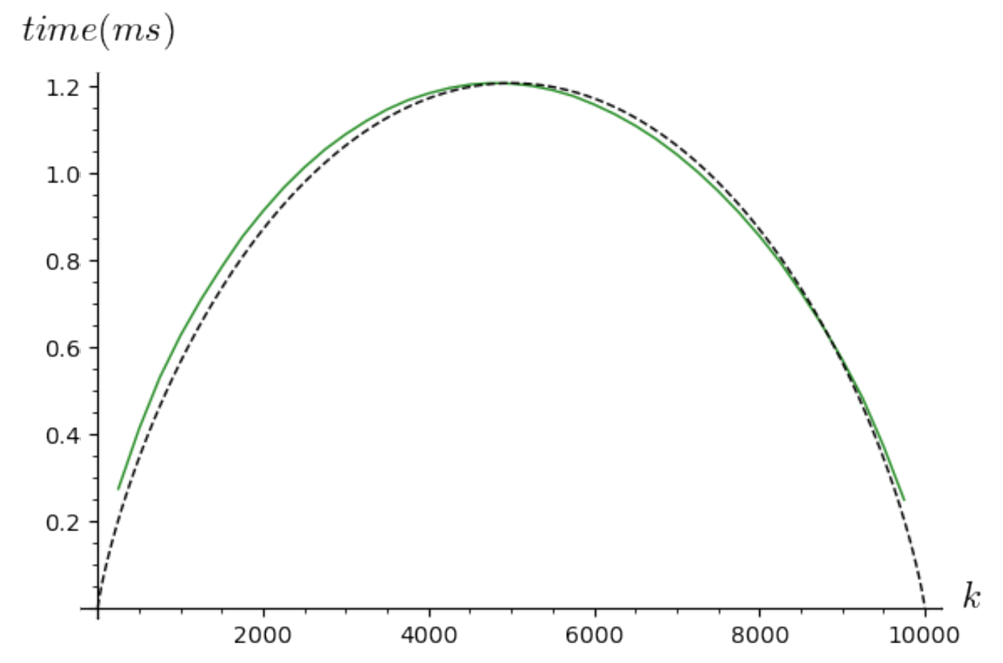
In Figure 4, we display the time complexity of our algorithm (in green) with the graph of the function where the constant C was chosen so that the maximum values of both curves coincide.
This validates experimentally our complexity results. Besides, we checked by profiling the optimized algorithms that most of the run time is spent in the arithmetic operations, which also confirms the validity of our complexity model.
5. Extensions of the Algorithmic Context
5.1. Objects Counted by Multinomial Coefficients
Let n and m be two positive integers and let be a finite sequence of non-negative integers whose sum equals n. The multinomial coefficient counts the number of ways of depositing n distinct objects into m distinct buckets such that there are objects in the ith bucket. It can also be interpreted as combination with repetitions as follows. Consider we have a (large enough) pool of m kinds of different objects and we must pick a finite sequence of n objects from this pool such that of them are of the first kind, of the second kind, and so on.
Note that, when , the multinomial coefficient corresponds to a binomial coefficient. Informally, Proposition 1 (related to combinations) states that combinations are in one-to-one correspondence with permutations containing two increasing runs. We have an analogous interpretation here. The ranks from 0 to are in one-to-one correspondence with size-n permutations composed of m increasing runs. We now exhibit this link more formally.
Proposition 4.
Let n and m be two positive integers and let be a sequence of non-negative integers such that . Each object enumerated by is represented by a finite sequence where for all , is an increasing finite sequence of length . Furthermore, the union over i of all elements of is exactly .
Our unranking algorithm relies on the classical formula expressing the multinomial coefficient as a product of binomial coefficients.
| Algorithm 8 Unranking a combination with repetitions. |
| 1: function UnrankingCombinationWithRepetitions() |
| 2: ▷n components in M |
| 3. |
| 4: |
| 5: for i from downto 1 do |
| 6: |
| 7: |
| 8: |
| 9: |
| 10: for j from 0 to do |
| 11: |
| 12: |
| 13: return |
| division: returns the pair corresponding respectively to the quotient and the remainder of |
| the integer division of s by t. |
Proposition 5.
The function UnrankingCombinationWithRepetitions computes the uth object counted by in lexicographic order.
The core of the algorithm consists in computing the rank of the permutation, written in factoradics, associated with the combination with repetitions we are interested in. It remains then to unrank a permutation.
Proof.
Based on Proposition 4, the core of the algorithm computes the rank of a permutation containing m increasing runs respectively of lengths . Determining the contribution of each run in the factoradic decomposition of the permutation rank is done in the external loop starting in Line 5, from down to . The correctness of our algorithm relies on the following loop invariant:
- The values of for all have been computed and stored in F.
- The values of (which has not been determined yet, as we enter the loop) are equal to the factoradics of the rank in the combinations of elements among possible elements.
- The variable holds the rank of the runs that must be still unranked.
□
Once the factoradic of the run under consideration has been computed (Line 10), it remains to update F according to the last components of .
5.2. Objects Counted by k-Permutations
Let n and k be two positive integer. A k-permutation is given by a combination of k elements among n elements, and an ordering of these k elements. The number of k-permutation over a set of n elements is given by:
Proposition 6.
The function UnrankingKPermutation returns the result of a call to UnrankingCombinationWithRepetitions. Thus, it computes the uth k-permutation among n elements in lexicographic order.
Proof.
The facts that both combinatorial classes have the same cardinality and that the algorithm for unranking combination with repetitions is lexicographic induce the correctness of the function. □
6. Conclusions
In the present article, we first exhibit, in Section 2, a new algorithm based on the classical factoradic numeral system for the lexicographic unranking of combinations. We also give a first step complexity analysis of the algorithm.
Section 3 is dedicated to the survey of three classical algorithms. The first one is the algorithm based on the so-called recursive method. The other two algorithms are based on combinadics, which is a numeral system particularly suited to representing combinations. To the best of our knowledge, it is the first time that both algorithms are compared. During the survey, we extend our complexity analysis based on a generating function approach, as presented in Section 2, in order to obtain a uniform presentation of the analysis of all four algorithms. Obviously, we thus reprove their average complexity results but with more details. Then, in Section 4, we compare their efficiency experimentally and propose a way to improve all these algorithms based on classical formulas of the binomial coefficient.
As a surprising result, we find that all the usual algorithms share a very similar core, doing almost the same computations in order to reconstruct the combination under consideration.
One interesting remark is that understanding in detail the core computations that are necessary to unrank combinations, it is possible to significantly improve all algorithms. This understanding, joined with a detailed and realistic theoretical complexity analysis, leads to a prediction of the run time of the algorithm that closely matches the actual run time of their implementations.
However, due to details that are neglected in practice, we realize in Table 1 that some improvements are still necessary in various computer algebra systems in order to get the most efficient implementations possible for the unranking of combinatorial objects.
Finally, in Section 5, we extend our approach to solve the problem of unranking structures enumerated by multinomial coefficients and objects counted by the k-permutations of n elements (also called arrangements).
Author Contributions
The authors contributed equally to this work. All authors have read and agreed to the published version of the manuscript.
Funding
This research received no external funding.
Data Availability Statement
Publicly available datasets were analyzed in this study. This data can be found here: http://github.com/Kerl13/combination_unranking (accessed on 15 March 2021).
Acknowledgments
The authors thank C. Donnot and Y. Herida for having conducted the preliminary experiments about our algorithm. Furthermore, the authors thank the referees for their careful reading of the paper, their comments and suggested improvements.
Conflicts of Interest
The authors declare no conflict of interest.
References
- Shablya, Y.; Kruchinin, D.; Kruchinin, V. Method for Developing Combinatorial Generation Algorithms Based on AND/OR Trees and Its Application. Mathematics 2020, 8, 962. [Google Scholar] [CrossRef]
- Grebennik, I.; Lytvynenko, O. Developing software for solving some combinatorial generation and optimization problems. In Proceedings of the 7th International Conference on Application of Information and Communication Technology and Statistics in Economy and Education, Sofia, Bulgaria, 3–4 November 2017; pp. 135–143. [Google Scholar]
- Tamada, Y.; Imoto, S.; Miyano, S. Parallel Algorithm for Learning Optimal Bayesian Network Structure. J. Mach. Learn. Res. 2011, 12, 2437–2459. [Google Scholar]
- Myers, A.F. k-out-of-n:G System Reliability With Imperfect Fault Coverage. IEEE Trans. Reliab. 2007, 56, 464–473. [Google Scholar] [CrossRef]
- Bodini, O.; Genitrini, A.; Naima, M. Ranked Schröder Trees. In Proceedings of the Sixteenth Workshop on Analytic Algorithmics and Combinatorics, ANALCO 2019, San Diego, CA, USA, 6 January 2019; pp. 13–26. [Google Scholar] [CrossRef] [Green Version]
- Ali, N.; Shamoon, A.; Yadav, N.; Sharma, T. Peptide Combination Generator: A Tool for Generating Peptide Combinations. ACS Omega 2020, 5, 5781–5783. [Google Scholar] [CrossRef] [PubMed]
- Ruskey, F. Combinatorial Generation; 2003; (unpublished); Available online: https://citeseerx.ist.psu.edu/viewdoc/summary?doi=10.1.1.93.5967 (accessed on 15 March 2021).
- Knuth, D.E. The Art of Computer Programming, Volume 4A, Combinatorial Algorithms; Addison-Wesley Professional: Boston, MA, USA, 2011. [Google Scholar]
- Skiena, S. The Algorithm Design Manual, Third Edition; Texts in Computer Science; Springer: Berlin/Heidelberg, Germany, 2020. [Google Scholar] [CrossRef]
- Ryabko, B.Y. Fast enumeration of combinatorial objects. Discret. Math. Appl. 1998, 8, 163–182. [Google Scholar] [CrossRef] [Green Version]
- Nijenhuis, A.; Wilf, H.S. Combinatorial Algorithms; Computer Science and Applied Mathematics; Academic Press: New York, NY, USA, 1975. [Google Scholar]
- Flajolet, P.; Zimmermann, P.; Van Cutsem, B. A calculus for the random generation of labelled combinatorial structures. Theor. Comput. Sci. 1994, 132, 1–35. [Google Scholar] [CrossRef]
- Martínez, C.; Molinero, X. A generic approach for the unranking of labeled combinatorial classes. Random Struct. Algorithms 2001, 19, 472–497. [Google Scholar] [CrossRef] [Green Version]
- Kokosinski, Z. Algorithms for Unranking Combinations and their Applications. In Proceedings of the Seventh IASTED/ISMM International Conference on Parallel and Distributed Computing and Systems, Washington, DC, USA, 19–21 October 1995; Hamza, M.H., Ed.; IASTED/ACTA Press: Calgary, AB, Canada, 1995; pp. 216–224. [Google Scholar]
- Pascal, E. Sopra una formula numerica. G. Di Mat. 1887, 25, 45–49. [Google Scholar]
- Beckenbach, E.F.; Pólya, G. Applied Combinatorial Mathematics; R.E. Krieger Publishing Company: Malabar, FL, USA, 1981. [Google Scholar]
- Laisant, C.A. Sur la numération factorielle, application aux permutations. Bull. Soc. Math. Fr. 1888, 16, 176–183. [Google Scholar] [CrossRef] [Green Version]
- Fisher, R.A.; Yates, F. Statistical Tables for Biological, Agricultural and Medical Research; Oliver & Boyd: London, UK, 1948. [Google Scholar]
- Bonet, B. Efficient algorithms to rank and unrank permutations in lexicographic order. In AAAI Workshop on Search in AI and Robotics—Technical Report; The AAAI Press: Menlo Park, CA, USA, 2008; pp. 142–151. [Google Scholar]
- Bodini, O.; Genitrini, A.; Peschanski, F. A Quantitative Study of Pure Parallel Processes. Electron. J. Comb. 2016, 23, 39. [Google Scholar] [CrossRef]
- Durstenfeld, R. Algorithm 235: Random Permutation. Commun. ACM 1964, 7, 420. [Google Scholar] [CrossRef]
- Buckles, B.P.; Lybanon, M. Algorithm 515: Generation of a Vector from the Lexicographical Index [G6]. ACM Trans. Math. Softw. 1977, 3, 180–182. [Google Scholar] [CrossRef]
- Er, M.C. Lexicographic ordering, ranking and unranking of combinations. Int. J. Comput. Math. 1985, 17, 277–283. [Google Scholar] [CrossRef]
- Flajolet, P.; Sedgewick, R. Analytic Combinatorics; Cambridge University Press: Cambridge, UK, 2009. [Google Scholar]
- Flajolet, P.; Sedgewick, R. An Introduction to the Analysis of Algorithms, 2nd ed.; Addison Wesley: Boston, MA, USA, 2013. [Google Scholar]
- Kreher, D.L.; Stinson, D.R. Combinatorial Algorithms: Generation, Enumeration, and Search; CRC Press: Boca Raton, FL, USA, 1999. [Google Scholar]
- McCaffrey, J. Generating the mth Lexicographical Element of a Mathematical Combination. MSDN. 2004. Available online: http://docs.microsoft.com/en-us/previous-versions/visualstudio/aa289166(v=vs.70) (accessed on 15 March 2021).
- The Sage Developers. SageMath, the Sage Mathematics Software System (Version 9.2). 2020. Available online: https://www.sagemath.org/ (accessed on 15 March 2021).
- Butler, B. Function kSubsetLexUnrank, MATLAB Central File Exchange. 2015. Available online: http://fr.mathworks.com/matlabcentral/fileexchange/53976-combinatorial-numbering-rank-and-unrank (accessed on 15 March 2021).
- Bostan, A.; Chyzak, F.; Giusti, M.; Lebreton, R.; Lecerf, G.; Salvy, B.; Schost, E. Algorithmes Efficaces en Calcul Formel, 10th ed.; Printed by CreateSpace: Palaiseau, France, 2017; 686p. [Google Scholar]
Figure 1.
Time (in ms) for unranking a combination, with n = 250…10,000 and .

Figure 2.
Time (in ms) for unranking a combination with the optimized algorithms.

Figure 3.
Time (in ms) for unranking a combination, with 10,000 and k = 25…9975.

Figure 4.
Merge of Algorithm 2 and its theoretical complexity.


Table 1.
Average time (in ms) for the unranking of a combination of k elements among n (too long means that the average time is larger than 30,000 ms).
Table 1.
Average time (in ms) for the unranking of a combination of k elements among n (too long means that the average time is larger than 30,000 ms).
| Time in ms | ||||||||||
|---|---|---|---|---|---|---|---|---|---|---|
| Sample | Sagemath | Maple | Mathematica | Matlab | ||||||
| Our Algo. | v. 9.0 | v. 9.2 | v. 2020.0 | v. 12.1.1.0 | v. R2020b | |||||
| Implem. | in C | Their Algo. | New Algo. | Their Algo. | Our Algo. | Their Algo. | Our Algo. | Their Algo. | Our Algo. | |
| 0.05464 | 2.6045 | 2.9672 | 78.2 | 2.12 | 0.44176 | 4.3145 | 3996.6 | 3041.2 | ||
| 0.06052 | 8.8903 | 2.4784 | 614 | 2.96 | 0.34608 | 3.9547 | 3520.6 | 3380.0 | ||
| 0.17496 | 15.8968 | 8.7929 | 1180 | 13.2 | 5.9131 | 11.823 | 11,846 | 9315.2 | ||
| 0.27524 | 96.3589 | 8.0500 | 6130 | 19.2 | 4.9624 | 13.067 | 11,087 | 9879.4 | ||
| 10,000 | 1.2554 | 191.03 | 31.665 | too long | 65.1 | 21.906 | 39.935 | too long | too long | |
| 10,000 | 2.3849 | 2245.6 | 29.027 | too long | 97.9 | 29.916 | 46.452 | too long | too long | |
Table 2.
First values of for and (Algorithm 2).
| k | 0 | 1 | 2 | 3 | 4 | 5 | 6 | 7 | 8 | |
|---|---|---|---|---|---|---|---|---|---|---|
| n | ||||||||||
| 1 | 0 | 1 | ||||||||
| 2 | 0 | 3 | 2 | |||||||
| 3 | 0 | 6 | 8 | 3 | ||||||
| 4 | 0 | 10 | 20 | 15 | 4 | |||||
| 5 | 0 | 15 | 40 | 45 | 24 | 5 | ||||
| 6 | 0 | 21 | 70 | 105 | 84 | 35 | 6 | |||
| 7 | 0 | 28 | 112 | 210 | 224 | 140 | 48 | 7 | ||
| 8 | 0 | 36 | 168 | 378 | 504 | 420 | 216 | 63 | 8 | |
Table 3.
First values of for and (Algorithm 3).
| k | 0 | 1 | 2 | 3 | 4 | 5 | 6 | 7 | 8 | |
|---|---|---|---|---|---|---|---|---|---|---|
| n | ||||||||||
| 1 | 0 | 0 | ||||||||
| 2 | 0 | 2 | 0 | |||||||
| 3 | 0 | 5 | 5 | 0 | ||||||
| 4 | 0 | 9 | 16 | 9 | 0 | |||||
| 5 | 0 | 14 | 35 | 35 | 14 | 0 | ||||
| 6 | 0 | 20 | 64 | 90 | 64 | 20 | 0 | |||
| 7 | 0 | 27 | 105 | 189 | 189 | 105 | 27 | 0 | ||
| 8 | 0 | 35 | 160 | 350 | 448 | 350 | 160 | 35 | 0 | |
Table 4.
Combinadics and their combinations for and .
| Rank, u | Reversed Rank, | Combinadic of | Combination of Rank u |
|---|---|---|---|
| 0 | 14 | (4, 5) | (0, 1) |
| 1 | 13 | (3, 5) | (0, 2) |
| 2 | 12 | (2, 5) | (0, 3) |
| 3 | 11 | (1, 5) | (0, 4) |
| 4 | 10 | (0, 5) | (0, 5) |
| 5 | 9 | (3, 4) | (1, 2) |
| 6 | 8 | (2, 4) | (1, 3) |
| 7 | 7 | (1, 4) | (1, 4) |
| 8 | 6 | (0, 4) | (1, 5) |
| 9 | 5 | (2, 3) | (2, 3) |
| 10 | 4 | (1, 3) | (2, 4) |
| 11 | 3 | (0, 3) | (2, 5) |
| 12 | 2 | (1, 2) | (3, 4) |
| 13 | 1 | (0, 2) | (3, 5) |
| 14 | 0 | (0, 1) | (4, 5) |
Table 5.
First values of for and (Algorithm 4).
| k | 0 | 1 | 2 | 3 | 4 | 5 | 6 | 7 | 8 | |
|---|---|---|---|---|---|---|---|---|---|---|
| n | ||||||||||
| 1 | 1 | 2 | ||||||||
| 2 | 1 | 5 | 3 | |||||||
| 3 | 1 | 9 | 11 | 4 | ||||||
| 4 | 1 | 14 | 26 | 19 | 5 | |||||
| 5 | 1 | 20 | 50 | 55 | 29 | 6 | ||||
| 6 | 1 | 27 | 85 | 125 | 99 | 41 | 7 | |||
| 7 | 1 | 35 | 133 | 245 | 259 | 161 | 55 | 8 | ||
| 8 | 1 | 44 | 196 | 434 | 574 | 476 | 244 | 71 | 9 | |
Table 6.
First values of for and (Algorithm 5).
| k | 0 | 1 | 2 | 3 | 4 | 5 | 6 | 7 | 8 | |
|---|---|---|---|---|---|---|---|---|---|---|
| n | ||||||||||
| 1 | 0 | 0 | ||||||||
| 2 | 0 | 0 | 1 | |||||||
| 3 | 0 | 0 | 4 | 2 | ||||||
| 4 | 0 | 0 | 10 | 10 | 3 | |||||
| 5 | 0 | 0 | 20 | 30 | 18 | 4 | ||||
| 6 | 0 | 0 | 35 | 70 | 63 | 28 | 5 | |||
| 7 | 0 | 0 | 56 | 140 | 168 | 112 | 40 | 6 | ||
| 8 | 0 | 0 | 84 | 252 | 378 | 336 | 180 | 54 | 7 | |
Publisher’s Note: MDPI stays neutral with regard to jurisdictional claims in published maps and institutional affiliations. |
© 2021 by the authors. Licensee MDPI, Basel, Switzerland. This article is an open access article distributed under the terms and conditions of the Creative Commons Attribution (CC BY) license (http://creativecommons.org/licenses/by/4.0/).
Share and Cite
MDPI and ACS Style
Genitrini, A.; Pépin, M. Lexicographic Unranking of Combinations Revisited. Algorithms 2021, 14, 97. https://0-doi-org.brum.beds.ac.uk/10.3390/a14030097
AMA Style
Genitrini A, Pépin M. Lexicographic Unranking of Combinations Revisited. Algorithms. 2021; 14(3):97. https://0-doi-org.brum.beds.ac.uk/10.3390/a14030097
Chicago/Turabian StyleGenitrini, Antoine, and Martin Pépin. 2021. "Lexicographic Unranking of Combinations Revisited" Algorithms 14, no. 3: 97. https://0-doi-org.brum.beds.ac.uk/10.3390/a14030097
Note that from the first issue of 2016, this journal uses article numbers instead of page numbers. See further details here.