
Chaos and Stability in a New Iterative Family for Solving Nonlinear Equations


Institute for Multidisciplinary Mathematics, Universitat Politècnica de València, Camino de Vera s/n, 46022 València, Spain
*
Author to whom correspondence should be addressed.
Algorithms 2021, 14(4), 101; https://0-doi-org.brum.beds.ac.uk/10.3390/a14040101
Submission received: 10 March 2021
/
Revised: 22 March 2021
/
Accepted: 23 March 2021
/
Published: 24 March 2021
(This article belongs to the Special Issue 2021 Selected Papers from Algorithms Editorial Board Members)
Abstract
:In this paper, we present a new parametric family of three-step iterative for solving nonlinear equations. First, we design a fourth-order triparametric family that, by holding only one of its parameters, we get to accelerate its convergence and finally obtain a sixth-order uniparametric family. With this last family, we study its convergence, its complex dynamics (stability), and its numerical behavior. The parameter spaces and dynamical planes are presented showing the complexity of the family. From the parameter spaces, we have been able to determine different members of the family that have bad convergence properties, as attracting periodic orbits and attracting strange fixed points appear in their dynamical planes. Moreover, this same study has allowed us to detect family members with especially stable behavior and suitable for solving practical problems. Several numerical tests are performed to illustrate the efficiency and stability of the presented family.
1. Introduction
Many problems in Computational Sciences and other disciplines can be stated in the form of a nonlinear equation or nonlinear systems using mathematical modeling. In particular, a large number of problems in Applied Mathematics and Engineering are solved by finding the solutions of these equations.
In the literature, there are many methods and families of iterative schemes that have been designed by using different procedures to approximate the simple roots of a nonlinear equation , where is a real function defined in an open interval I. We can find in [1,2,3] several surveys and overviews of the iterative schemes published in the last years. Each method has a different behavior. This behavior is characterized with the efficiency criteria and the complex dynamics tools.
In this paper, we introduce a new family of multistep iterative schemes to solve nonlinear equations, which contains as an element of this family, a particular method presented in [4]. This family is built from the Ostrowski’s scheme, adding a Newton step with a “frozen” derivative and using a divided difference operator. Therefore, the family has a three-step iterative expression. Furthermore, it has three arbitrary parameters named , , and , which can take real or complex values, and an order of convergence of at least four. The order of convergence will be discussed in Section 2.
From the error equation we observe by fixing two parameters in function of the third one, an uniparametric family of sixth-order iterative methods is obtained. We analyze the dynamical behavior of this family in terms of values of the parameter, in order to detect its elements with good stability properties and others with chaotic behavior. The concept of chaos has been widely discussed (see, for example, in [5]) and it is commonly understood as the presence of complex orbit structure and extreme sensitivity of orbits to small perturbations. Moreover, the presence of unstable periodic orbits of all periods is also included in the concept of chaotic system. For this study, we use tools of discrete complex dynamics that we introduce in Section 3.
In Section 4, we present the performance of the presented schemes on several test functions. These numerical tests allow us to confirm the results obtained in the dynamical section and to compare our schemes with other known ones. The manuscript finishes with some conclusions and the references used in it.
The parametric family object of study in this manuscript has the following iterative expression:
where ; ; ; and , , and are arbitrary parameters.
The divided difference operator defined by Ortega and Rheinboldt in [6], satisfies
2. Convergence of the New Family
In this section, we perform the convergence analysis of the new triparametric iterative family. Furthermore, we propose a strategy to reduce the triparametric scheme to an uniparametric scheme in order to accelerate the convergence.
Theorem 1.
Let be a sufficiently differentiable function on an open interval I and a simple root of the nonlinear equation . Suppose that is continuous and sufficiently differentiable in an environment of the simple root ξ, and is an initial estimate close enough to ξ. Then, the sequence obtained by using the expression (1) converges to ξ with an order of convergence of four, being its error equation
where , and
Proof
Let be a simple root of (that is, and ) and . Using Taylor expansion of and around , we have
and
where ,
Dividing (3) by (4), we get
Replacing (5) in the first step of family (1), we have
Using Taylor expansion again, similar to (3), to develop around , we get
With (3), (6), and (7), we calculate the divided difference operator defined in (2), obtaining
Then, substituting (3), (4), (6), and (8) in the second step of family (1), we have
Using Taylor series once again, similar to (3), to expand around , we get
Replacing (4) and (8) in and of family (1), we have
Finally, substituting (4), (9)–(12) in the third step of family (1), we get
being the error equation
and the proof is finished. □
From Theorem 1, it follows that the new triparametric family of iterative methods has an order of convergence of four for any real or complex values of the parameters , , and . However, convergence can be speed-up if only one parameter is held and the family is reduced to an uniparametric iterative scheme. The latter can be seen in Theorem 2.
Theorem 2.
Let be a sufficiently differentiable function on an open interval I and a simple root of the nonlinear equation . Suppose that is continuous and sufficiently differentiable in an environment of the simple root ξ, and is an initial estimate close enough to ξ. Then, the sequence obtained by using the expression (1) converges to ξ with an order of convergence of six, provided that and , being its error equation
where , and
Proof
Let be a simple root of (that is, and ) and . Using Taylor expansion of and around , we have
and
where ,
Dividing (15) by (16), we get
Replacing (17) in the first step of family (1), we have
Using Taylor expansion again, similar to (15), to expand around , we get
With (15), (18), and (19), we calculate the divided difference operator defined in (2), obtaining
Then, substituting (15), (16), (18), and (20) in the second step of family (1), we have
Using Taylor series once again, similar to (15), to expand around , we get
Replacing (16) and (20) in and of family (1), we have
Finally, substituting (16) and (21)–(24) in the third step of family (1), we get
being the error equation
To cancel the factors accompanying and in (26), it must be satisfied that , and . It is easy to show that this system of equations has infinite solutions for
where is a free parameter. Therefore, replacing (27) in (26), we obtain
and the proof is finished. □
From Theorem 2, it follows that, if we only hold parameter in (1), the new triparametric family of iterative methods is reduced to an uniparametric family with an order of convergence of six for any real or complex values of the parameters , and , as long as (27) is satisfied. Therefore, the iterative expression of the new uniparametric family, dependent only on parameter and which we will call CMT() family, is defined as
where , , and
Because of the results obtained with the convergence analysis carried out, from now on we will only work with CMT() family of iterative methods and, to select the best members of this family, we will use the complex dynamics tools discussed in Section 3.
3. Complex Dynamics Behavior
This topic refers to the study of the behavior of a rational function associated with an iterative family or method. From the numerical point of view, the dynamical properties of the referred rational function give us important information about its stability and reliability. The parameter spaces of a family of methods, built from the critical points, allow us to understand the performance of the different members of the family, helping us in the election of a particular one. The dynamical planes show the behavior of these particular methods in terms of the basins of attraction of their fixed points, periodic points, etc. A basin of attraction provides us to visually interpret how a method works based on several initial estimates.
In this section, we present the study of the complex dynamics of CMT () family given in (29). To do this, we construct a rational operator associated with the family, on a generic low-degree nonlinear polynomial, and we analyze the stability and convergence of the corresponding fixed and critical points. Then, we construct the parameter spaces of the free critical points and generate dynamical planes of some methods of the family for good and bad values of , in terms of stability.
3.1. Rational Operator
The rational operator can be built on any nonlinear function; however, we construct this operator on quadratic polynomials, as the criterion of stability or instability of a method applied to these polynomials can be generalized for other nonlinear functions.
Proposition 1.
Let be a generic quadratic polynomial with roots . Therefore, the rational operator associated with CMT(α) family given in (29) and applied on , is
with an arbitrary parameter. Furthermore, if , is simplified as shown
Proof
Let be a generic quadratic polynomial with roots . We apply the iterative scheme given in (29) on and obtain a rational function which depends on the roots and a parameter . Then, if we use Möbius transformation (see in [7,8,9]) in with
that satisfies and , we get
which only depends on an arbitrary parameter . Furthermore, if we factor numerator and denominator of (35), it is easy to show that for some roots coincide and simplify , as it is observed in Equations (31)–(34), and the proof is finished. □
From Proposition 1, for four values of the rational operator is simpler, so there will be fewer fixed and critical points that can improve the stability of the associated methods. This will be seen in Section 3.2 and Section 3.3.
3.2. Analysis and Stability of Fixed Points
We calculate the fixed points of the rational operator given in (30) and analyze their stability.
Proposition 2.
The fixed points of are the roots of the equation . That is, , and the following strange fixed points:
- (if ), and
- that correspond to the 10 roots of polynomial , where .
The total number of different fixed points varies with the value of α:
- If and , then has 13 fixed points.
- If , then is not a fixed point and has 12 fixed points.
- If , then has 11 fixed points.
- If , then and has 11 fixed points.
The pairs of conjugated strange fixed points, satisfying for , are and , and , and , and , and and .
From Proposition 2, we establish there is a minimum of 11 and a maximum of 13 fixed points. Of these, 0 and ∞ correspond to the roots of the original quadratic polynomial , and the strange fixed point (if ) corresponds to the divergence of the original method, before Möbius transformation.
Proposition 3.
The stability of the strange fixed point , , verifies:
- (i)
- If , then is an attractor.
- (ii)
- If , then is a repulsor.
- (iii)
- If , then is parabolic.
is never a superattractor because . The superattracting fixed points that satisfy are , and the following strange fixed points:
- , for ,
- , for , and
- , for .
The repulsive fixed points, which always satisfy , are the strange fixed points and .
It is clear that 0 and ∞ are always superattracting fixed points, but the stability of the rest of fixed points depends on the values of parameter . From Proposition 3, there are 6 strange fixed points that can become superattractors for certain values of . This means that there would be a basin of attraction of the strange fixed point and it could cause the method not to converge to the solution.
Figure 1 shows the stability surface of the strange fixed point . In this figure, the zones of attraction (yellow surface) and repulsion (gray surface) are observed, being the first one much greater than the second one. Note that for values of inside disk, is a repulsor; and, for off-disk values of , is an attractor. Therefore, it is in our interest to always work inside the disk because the strange fixed point comes from the divergence of the original method and, therefore, it is better for the performance of the iterative method that the divergence is repulsive.
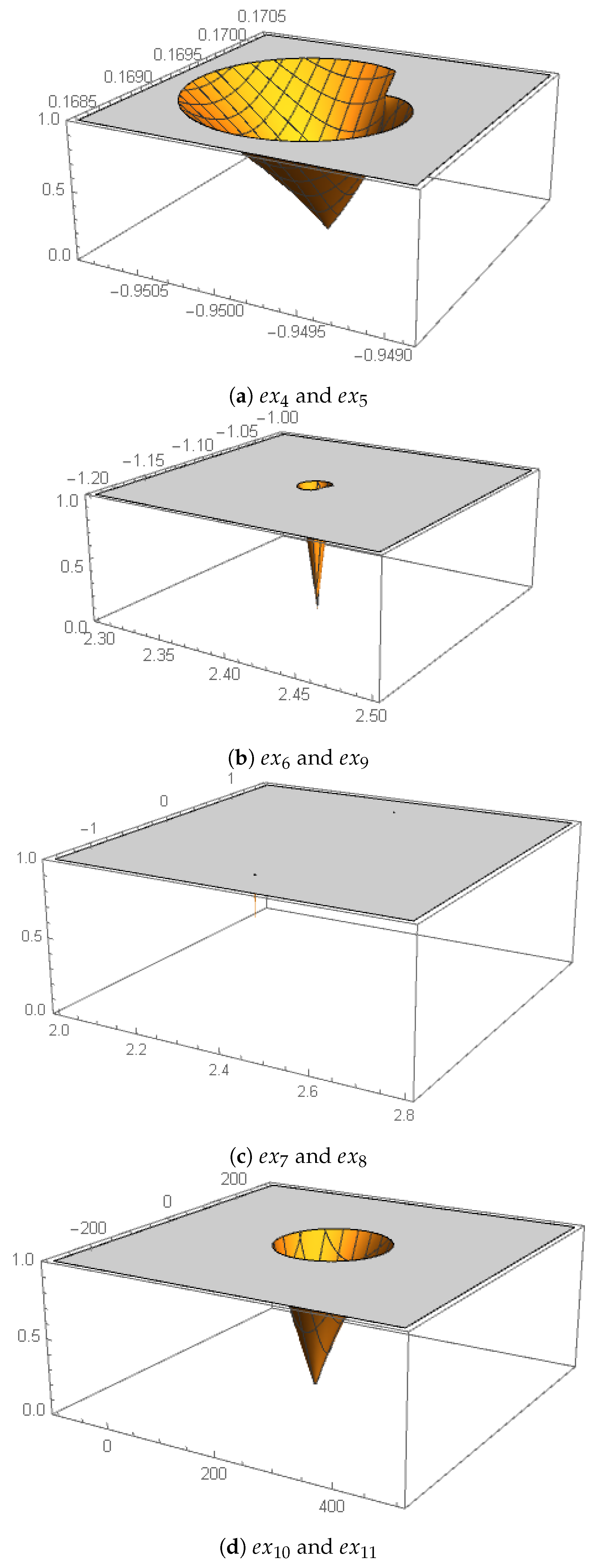
From Proposition 2, the study of the stability of strange fixed points is reduced by a half. This is because each pair of conjugated strange fixed points exhibits the same stability characteristics. Furthermore, due to Proposition 3, and are always repulsors regardless of the value of . Thus, Figure 2 shows the stability surfaces of the remaining 8 strange fixed points, which can be attracting or repulsive depending on the value of , for analysis.
3.3. Analysis of Critical Points
We calculate the critical points of the rational operator given in (30).
Proposition 4.
The critical points of are the roots of the equation . That is, , and the following free critical points:
- ,
- ,
- , and
- that correspond to the 6 roots of polynomial , where .
The total number of different critical points varies with the value of α:
- If and , then has 11 critical points.
- If , then is simplified or reduced and has 9 critical points.
- If , then is simplified and has 7 critical points.
The pairs of conjugated free critical points, satisfying for , are and , and , and , and and .
From Proposition 4, we establish there is a minimum of 7 and a maximum of 11 critical points. Of these, 0 and ∞ correspond to the roots of the original quadratic polynomial . The free critical points , , and are pre-images of the strange fixed point . Therefore, the stability of , , and will correspond to the stability of (see Section 3.2). Moreover, the dynamical study of the free critical points is reduced by a half because each pair of conjugated free critical points presents the same stability characteristics. This will be seen in Section 3.4.
3.4. Parameter Spaces
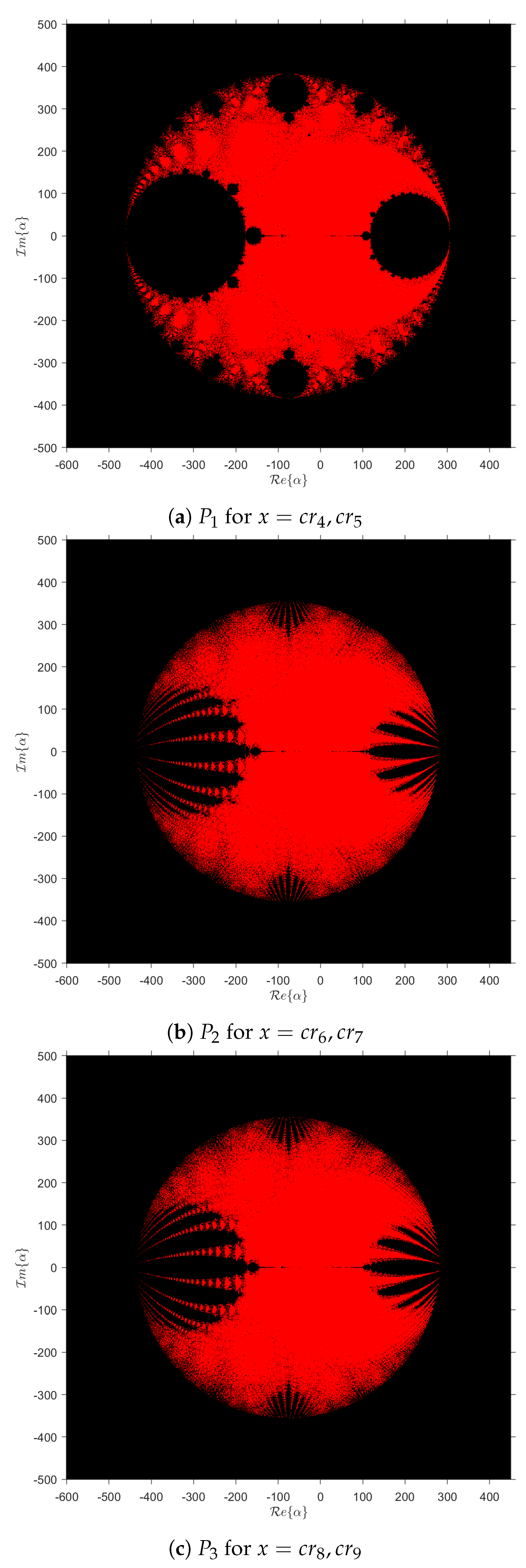
The dynamical behavior of operator depends on the values of parameter . The parameter space is defined as a mesh in the complex plane where each point of this mesh corresponds to a different value of . Its graphical representation shows the convergence analysis of a method of CMT () family associated with this using one of the free critical points given in Proposition 4 as initial estimate. The resulting graphic is made in Matlab R2020a programming package with a resolution of 1000 × 1000 pixels. If a method converges to any of the roots starting from in a maximum of 80 iterations with a tolerance of , the pixel is colored red; in other cases, the pixel is colored black.
Each value of that belongs to the same connected component of the parameter space results in subsets of schemas with similar dynamical behavior. Therefore, it is interesting to find regions of the parameter space as stable as possible (red regions), because these values of will give us the best members of the family in terms of numerical stability.
CMT() family has a maximum of 9 free critical points. Of these, , , and have the same parameter space which corresponds to the stability surface of (see Figure 1), because they are pre-images of this point. The remaining free critical points, to , are conjugated in pairs (see Proposition 4), which gives rise to 3 different parameter spaces. These parameter spaces, named (for ), (for ), and (for ), are shown in Figure 3.
From Figure 3b,c, we observe that the parameter spaces and have similar characteristics; then, we can select any of them for analysis.
On the one hand, if we choose values of inside the stability regions (red regions) of the parameter spaces, for example, , the methods associated with these parameters will show good dynamical behavior in terms of numerical stability. Furthermore, note that these particular values of simplify the iterative scheme of CMT() family given in (29) by canceling a term in its third step. This is especially useful to improve the computational efficiency of the associated method because the processing times required to reach the solution are reduced (see Section 4).
On the other hand, if we choose values of outside the stability regions (black regions) of the parameter spaces, for example , the methods associated with these parameters will show poor dynamical behavior in terms of numerical stability.
The methods associated with the values of treated above are discussed in Section 3.5.
3.5. Dynamical Planes
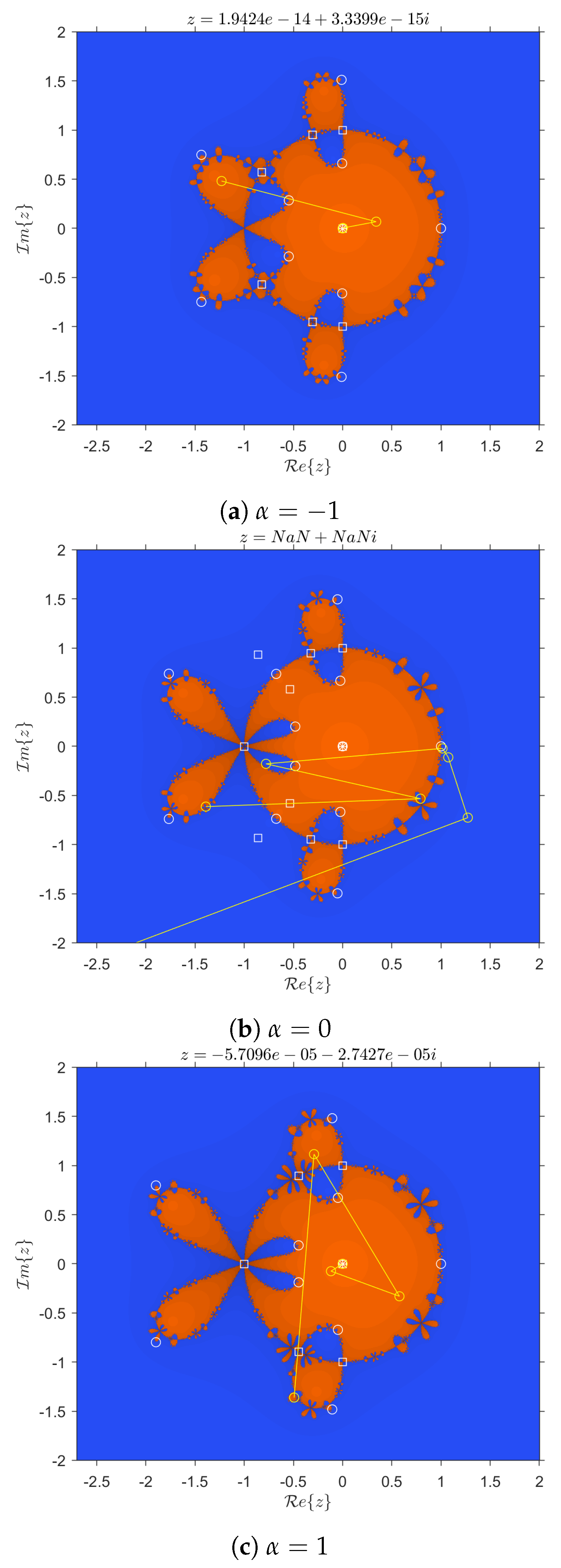
We begin this section by presenting how we generate a dynamical plane that will allow us to see the stability of a method for a specific value of . This is defined as a mesh in the complex plane where each point of this mesh corresponds to a different value of the initial estimate . Its graphical representation shows the convergence of the method to any of the roots starting from with a maximum of 50 iterations and a tolerance of . Fixed points are illustrated with a white circle “○”, critical points with a white square “□” and attractors with a white asterisk “∗”. Moreover, the basins of attraction are depicted in different colors. The resulting graphic is made in Matlab R2020a with a resolution of 1000 × 1000 pixels.
Here, we study the stability of some CMT() family methods through the use of dynamical planes. We will consider the methods proposed in Section 3.4 for values of inside and outside the stability regions of the parameter spaces.
On the one hand, examples of methods inside the stability region are given for . Their dynamical planes with some convergence orbits in yellow are shown in Figure 4. Note that all three methods present only two basins of attraction associated with the roots: the basin of 0 colored in orange and the basin of ∞ colored in blue. Furthermore, there are no black areas of non-convergence to the solution. Consequently, these methods show good dynamical behavior: they are very stable. Of these methods, the best member of CMT() family is for , as it has fewer strange fixed points and free critical points.
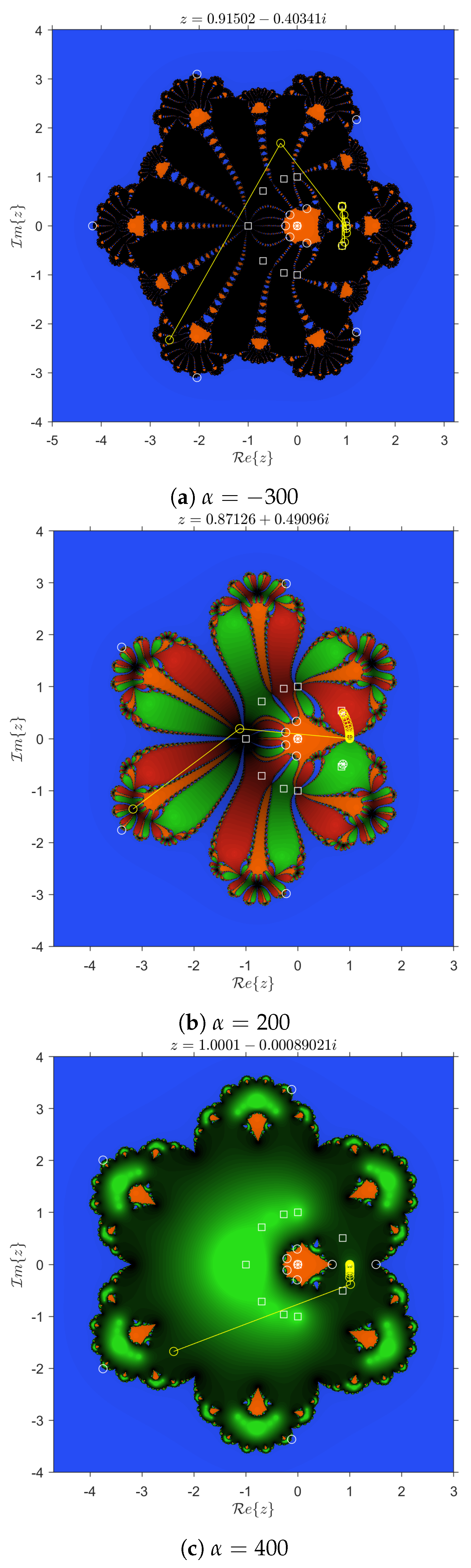
On the other hand, examples of methods outside the stability region are given for . Their dynamical planes with some convergence orbits in yellow are shown in Figure 5. Note that all three methods present more than two basins of attraction, that is, there are other basins of attraction that do not correspond to the roots. The basins of 0 and ∞ are colored in orange and blue, respectively, and the other basins are colored in black, red, and green. Figure 5a shows the convergence to an attracting periodic orbit of period 2. Figure 5b,c shows the convergence to an attracting strange fixed point. Furthermore, let us remark that in the three figures the basin of 0 is very small, due to the presence of the other basins of attraction, which reduces the chances of convergence to the solution. Likewise, there are black areas of slow convergence of the methods. Consequently, these methods have poor dynamical behavior: they are unstable.
4. Numerical Results
Here, we perform several numerical tests in order to check the theoretical convergence and stability results of CMT() family obtained in previous sections. To do this, we use some stable and unstable methods of (29). These methods are applied on five nonlinear test functions, whose expressions and corresponding roots are
Thus, we performed two experiments. In a first experiment, we carried out a efficiency analysis of CMT() family through a comparative study between one of its stable methods and five different methods given in the literature: Newton of order 2, Ostrowski of order 4, and three other methods of order 6 proposed by Alzahrani et al. in [10] (ABA), Chun and Ham in [11] (CH), and Amat et al. in [12] (AHR). In a second experiment, we carried out a stability analysis of CMT () family using six of its methods obtained with three good and three bad values of parameter , in terms of stability.
In the development of the numerical tests we start the iterations with different initial estimates: close (), far (), and very far () to the root , respectively. This allows us to measure, to some extent, how demanding the methods are relative to the initial estimation for finding a solution.
The calculations are developed in Matlab R2020a programming package using variable precision arithmetics with 200 digits of mantissa. For each method, we analyze the number of iterations (iter) required to converge to the solution, so that the stopping criteria or are satisfied. Note that represents the error estimation between two consecutive iterations and is the residual error of the nonlinear test function. This stopping criterium does not need the exact solution, on the contrary of absolute error, and differs from recent ones as CESTAC (see in [13]) in the absence of additional calculations or functional evaluations, as is needed for the following iteration and its absolute values is an efficient control element of the proximity to the exact root, where f is zero. Indeed, although a precision of one hundred exact digits is not usually necessary in the applications, we employ this value in the stopping criterium as it is useful to check the robustness and effectiveness of the numerical methods.
To check the theoretical order of convergence (p), we calculate the approximate computational order of convergence (ACOC) given by Cordero and Torregrosa in [14]. In the numerical results presented below, if the ACOC vector inputs do not stabilize their values throughout the iterative process, it is marked as “-”; and, if any of the methods used does not reach convergence in a maximum of 50 iterations, it is marked as “nc”.
To illustrate the computational efficiency of each used method, the processing time (tcpu) in seconds required by the iterative scheme to converge to the solution is measured. This value is determined as the arithmetic mean of 10 runs of the method.
4.1. First Experiment: Efficiency Analysis of CMT () Family
In this experiment, we carried out a comparative study between a stable method of CMT () family and the methods of Newton, Ostrowski, ABA, CH and AHR, in order to contrast their numerical performances in nonlinear equations. We consider as a stable member of CMT () family the method associated with , that is, CMT(1).
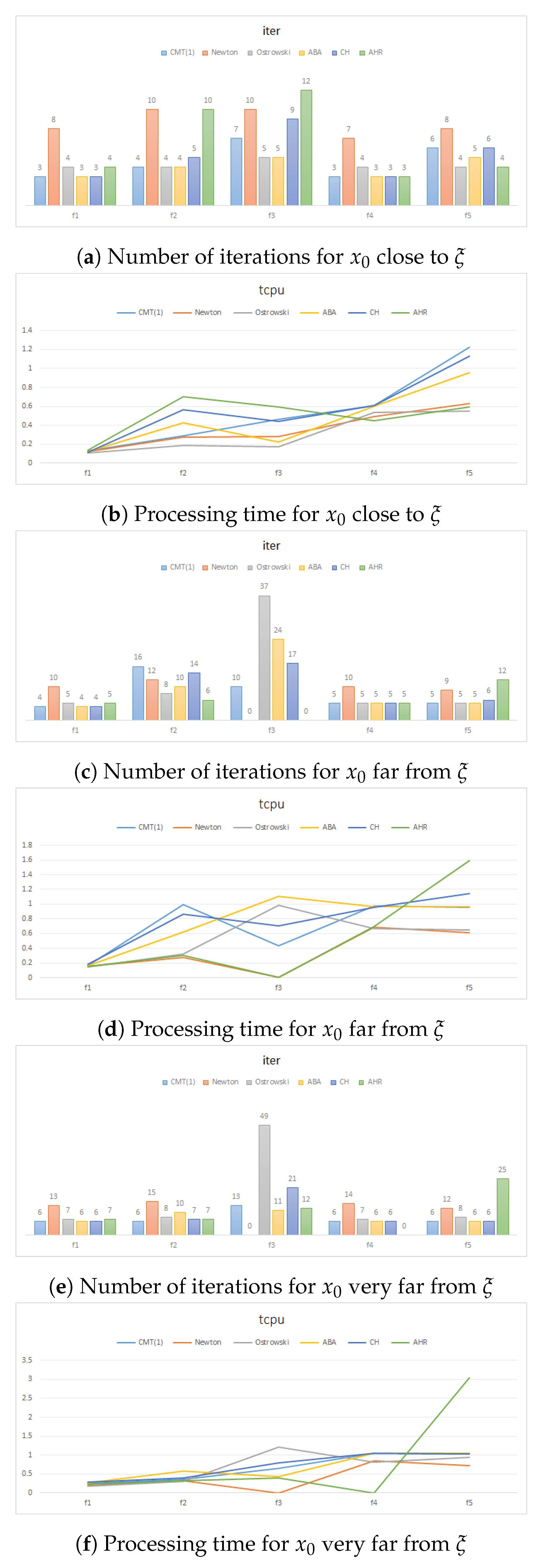
Thereby, in Table 1, Table 2 and Table 3 we show the numerical results of the six known methods, considering close, far, and very far initial estimates. Furthermore, in Figure 6 we show graphics that summarize these results for the number of iterations (iter) and the processing time (tcpu).
Therefore, from the results of the first experiment we conclude that CMT() family has an excellent numerical performance considering a stable member () as a representative. This conclusion has been made based on the following aspects from Table 1, Table 2 and Table 3: CMT (1) method has the lowest error and lowest number of iterations (iter). However, the mean of the execution time (tcpu) varies according to the nonlinear test function used and the inherent complexity that the iterative scheme of the method presents on the nonlinear function. In several cases, the tcpu of the CMT (1) method is significantly lower than the 6th order ABA, CH and AHR methods. The theoretical convergence order is also verified by the ACOC, which is close to 6.
4.2. Second Experiment: Stability Analysis of CMT() Family
In this experiment, we carried out a stability analysis of CMT () family considering some values of inside the stability regions of the parameter spaces () and outside of them ().
Thus, in Table 4, Table 5, Table 6, Table 7, Table 8 and Table 9 we show the numerical performance of iterative methods associated with these values of for close, far, and very far initial estimations. The results for were already presented in the first experiment; however, these are presented again due to the different conditions in which each experiment was performed.
On the one hand, from Table 4, Table 5 and Table 6 we observe that the methods associated with always converge to the solution, although the number of iterations (iter) needed differs for any initial estimate and nonlinear test function. Thus, in estimations close to the root, the methods converge to with a minimum iter of 3 and a maximum of 7. When the initial guess is far from the root, they converge to with a minimum iter of 4 and a maximum of 22. When the starting estimations are very far from the root, the iterative schemes converge to with a minimum iter of 6 and a maximum of 37.
On the other hand, from the results shown in Table 7, Table 8 and Table 9, we see that the methods associated with do not always converge to the solution, confirming the conclusions obtained in the dynamical analysis. The convergence highly depends on the initial estimation and the nonlinear test function used. Thus, for estimations close to the root, these methods do not converge to the solution in up to 2 test functions. Moreover, for estimations far and very far from the root, they do not converge to the solution even for any function.
Consequently, we conclude that the methods for are stable, have the lowest processing times (tcpu), and always converge to the solution for any initial estimate and nonlinear test function used. The methods for are unstable, chaotic, have the highest tcpu, and tend not to converge to the solution according to the initial estimate and the nonlinear test function used. With this, the theoretical results obtained in previous sections about the dynamical behavior of CMT() family are verified.
5. Conclusions
In this paper, a new family of iterative methods was designed to solve nonlinear equations from Ostrowski scheme, adding a Newton step with a “frozen” derivative and using a divided difference operator. This family, named CMT (), has a three-step iterative expression and three arbitrary parameters which can take any real or complex value.
In the convergence analysis of the new family, we obtained an order of convergence of four just like the order of the Ostrowski method. However, we managed to speed-up the convergence to six by setting the parameters and as a function of , resulting in an uniparametric CMT () family.
In the dynamical study, we constructed parameters spaces of the free critical points of the rational operator associated with the uniparametric family. These parameter spaces allowed us to understand the performance of the different members of the family, helping us to choose stable (for ) and unstable (for ) methods. Furthermore, we generated dynamical planes to show the behavior of these particular methods.
From numerical results, the order of convergence is verified by the ACOC, which is close to 6. The CMT () family proved to have an excellent numerical performance considering stable members as representatives. In general, this family has low errors and number of iterations to converge to the solution. However, the processing time (tcpu) varies depending on the nonlinear test functions used and the inherent complexity that the iterative schemes of the methods present when they are applied to said functions. In several cases, the tcpu of stable methods is significantly lower than other sixth-order methods developed so far. Furthermore, the methods for proved to be stable, have the lowest tcpu, and always converge to the solution for any initial estimate and nonlinear test function used. The methods for proved to be unstable, chaotic, have the highest tcpu, and tend not to converge to the solution according to the initial estimate and the nonlinear test function used. This verifies the theoretical results obtained in convergence analysis and dynamical study of CMT() family.
Author Contributions
Conceptualization, A.C. and J.R.T.; methodology, A.C. and M.M.-M.; software, M.M.-M.; validation, M.M.-M.; formal analysis, J.R.T.; investigation, A.C.; writing—original draft preparation, M.M.-M.; writing—review and editing, A.C.; supervision, J.R.T. All authors have read and agreed to the published version of the manuscript.
Funding
This research was partially supported by Ministerio de Ciencia, Innovación y Universidades PGC2018-095896-B-C22.
Institutional Review Board Statement
Not applicable.
Informed Consent Statement
Not applicable.
Data Availability Statement
Not applicable.
Acknowledgments
The authors would like to thank the anonymous reviewers for their comments and suggestions, as they have improved the final version of this manuscript.
Conflicts of Interest
The authors declare no conflict of interest.
References
- Neta, B. Numerical Methods for the Solution of Equations; Net-A-Sof: Monterey, CA, USA, 1983. [Google Scholar]
- Petković, M.; Neta, B.; Petković, L.; Džunić, J. Multipoint Methods for Solving Nonlinear Equations, 1st ed.; Academic Press: Boston, MA, USA, 2013. [Google Scholar]
- Amat, S.; Busquier, S. Advances in Iterative Methods for Nonlinear Equations; Springer: Cham, Switzerland, 2017. [Google Scholar]
- Artidiello, S.; Cordero, A.; Torregrosa, J.; Penkova, M. Design and multidimensional extension of iterative methods for solving nonlinear problems. Appl. Math. Comput. 2017, 293, 194–203. [Google Scholar] [CrossRef]
- Hunt, B.R.; Ott, E. Defining chaos. Chaos Interdiscip. J. Nonlinear Sci. 2015, 25. [Google Scholar] [CrossRef] [PubMed]
- Ortega, J.M.; Rheinboldt, W.C. Iterative Solution of Nonlinear Equations in Several Variables; Academic Press: New York, NY, USA, 1970. [Google Scholar]
- Scott, M.; Neta, B.; Chun, C. Basin attractors for various methods. Appl. Math. Comput. 2011, 218, 2584–2599. [Google Scholar] [CrossRef]
- Amat, S.; Busquier, S.; Plaza, S. Review of some iterative root—Finding methods from a dynamical point of view. SCIENTIA Ser. A Math. Sci. 2004, 10, 3–35. [Google Scholar]
- Blanchard, P. Complex analytic dynamics on the Riemann sphere. Bull. Am. Math. Soc. 1984, 11, 85–141. [Google Scholar] [CrossRef] [Green Version]
- Alzahrani, A.; Behl, R.; Alshomrani, A. Some higher-order iteration functions for solving nonlinear models. Appl. Math. Comput. 2018, 334, 80–93. [Google Scholar] [CrossRef]
- Chun, C.; Ham, Y. Some sixth-order variants of Ostrowski root-finding methods. Appl. Math. Comput. 2007, 193, 389–394. [Google Scholar] [CrossRef]
- Amat, S.; Hernández, M.; Romero, N. Semilocal convergence of a sixth order iterative method for quadratic equations. Appl. Numer. Math. 2012, 62, 833–841. [Google Scholar] [CrossRef]
- Noeiaghdam, S.; Sidorov, D.; Zamyshlyaeva, A.; Tynda, A.; Dreglea, A. A valid dynamical control on the reverse osmosis system using the CESTAC method. Mathematics 2021, 9, 48. [Google Scholar] [CrossRef]
- Cordero, A.; Torregrosa, J.R. Variants of Newton’s Method using fifth-order quadrature formulas. Appl. Math. Comput. 2007, 190, 686–698. [Google Scholar] [CrossRef]
Figure 1.
Stability surface of (in gray color, the complex area where the fixed point is repulsive, being attracting in the rest).
Figure 1.
Stability surface of (in gray color, the complex area where the fixed point is repulsive, being attracting in the rest).

Figure 2.
Stability surfaces of 8 strange fixed points (in gray color, the complex area where each fixed point is repulsive, being attracting in the rest).
Figure 2.
Stability surfaces of 8 strange fixed points (in gray color, the complex area where each fixed point is repulsive, being attracting in the rest).

Figure 3.
Parameter spaces of free critical points (in red color, the complex area where the corresponding critical point converges to 0 or ∞, that is, the stability region).
Figure 3.
Parameter spaces of free critical points (in red color, the complex area where the corresponding critical point converges to 0 or ∞, that is, the stability region).

Figure 4.
Dynamical planes for methods inside the stability region (basin of attraction of 0 in orange color; in blue color, the basin of ∞).
Figure 4.
Dynamical planes for methods inside the stability region (basin of attraction of 0 in orange color; in blue color, the basin of ∞).

Figure 5.
Dynamical planes for methods outside the stability region (basin of attraction of 0 in orange color; in blue color, the basin of ∞; in green or red color, the basin of attracting strange fixed points).
Figure 5.
Dynamical planes for methods outside the stability region (basin of attraction of 0 in orange color; in blue color, the basin of ∞; in green or red color, the basin of attracting strange fixed points).

Figure 6.
Numerical results of the first experiment.


Table 1.
Numerical performance of iterative methods in nonlinear equations for close to .
| Function | Method | iter | ACOC | tcpu | ||
|---|---|---|---|---|---|---|
| CMT(1) | 3 | 5.5148 | 0.1257 | |||
| −1.6 | Newton | 8 | 2 | 0.1225 | ||
| Ostrowski | 4 | 3.9988 | 0.1036 | |||
| ABA | 3 | 5.5472 | 0.1201 | |||
| CH | 3 | 5.5336 | 0.1173 | |||
| AHR | 0 | 4 | 5.9989 | 0.1381 | ||
| CMT(1) | 4 | 6.0717 | 0.2913 | |||
| −0.4 | Newton | 10 | 2 | 0.2747 | ||
| Ostrowski | 4 | 3.9993 | 0.1899 | |||
| ABA | 0 | 4 | 6.0055 | 0.4278 | ||
| CH | 5 | 5.9951 | 0.5636 | |||
| AHR | 0 | 10 | 5.9991 | 0.7038 | ||
| CMT(1) | 0 | 7 | 5.9957 | 0.4654 | ||
| 0.4 | Newton | 10 | 2 | 0.2818 | ||
| Ostrowski | 5 | 3.9999 | 0.1682 | |||
| ABA | 5 | 5.8933 | 0.224 | |||
| CH | 9 | 5.8498 | 0.4374 | |||
| AHR | 0 | 12 | 5.9521 | 0.5912 | ||
| CMT(1) | 1.2572 × 10⁻³² | 3 | 5.717 | 0.6075 | ||
| 1.3 | Newton | 7 | 2 | 0.4947 | ||
| Ostrowski | 4 | 4 | 0.535 | |||
| ABA | 3 | 5.9419 | 0.598 | |||
| CH | 3 | 5.6961 | 0.6046 | |||
| AHR | 3 | 5.6812 | 0.4497 | |||
| CMT(1) | 6 | 5.9132 | 1.2222 | |||
| −1.9 | Newton | 8 | 2 | 0.6295 | ||
| Ostrowski | 4 | 4.0146 | 0.5521 | |||
| ABA | 5 | 6.0107 | 0.9561 | |||
| CH | 6 | 6.2212 | 1.1314 | |||
| AHR | 4 | 5.7855 | 0.5939 |
Table 2.
Numerical performance of iterative methods in nonlinear equations for far from .
| Function | Method | iter | ACOC | tcpu | ||
|---|---|---|---|---|---|---|
| CMT(1) | 4 | 5.7093 | 0.163 | |||
| −6 | Newton | 10 | 2 | 0.1527 | ||
| Ostrowski | 5 | 3.9989 | 0.1487 | |||
| ABA | 4 | 5.775 | 0.1607 | |||
| CH | 4 | 5.7326 | 0.1811 | |||
| AHR | 0 | 5 | 5.9988 | 0.1578 | ||
| CMT(1) | 0 | 16 | 5.9975 | 0.9939 | ||
| −6 | Newton | 12 | 2 | 0.2714 | ||
| Ostrowski | 8 | 4 | 0.3234 | |||
| ABA | 10 | - | 0.6234 | |||
| CH | 0 | 14 | 5.9955 | 0.8618 | ||
| AHR | 0 | 6 | 5.9971 | 0.3006 | ||
| CMT(1) | 10 | 5.8416 | 0.4353 | |||
| −14 | Newton | nc | nc | nc | nc | nc |
| Ostrowski | 0 | 37 | 4 | 0.9868 | ||
| ABA | 24 | 6.2542 | 1.1023 | |||
| CH | 0 | 17 | 5.9997 | 0.7088 | ||
| AHR | nc | nc | nc | nc | nc | |
| CMT(1) | 5 | 5.9995 | 0.978 | |||
| −23 | Newton | 10 | 2 | 0.683 | ||
| Ostrowski | 5 | 3.9956 | 0.6646 | |||
| ABA | 5 | 5.9961 | 0.9691 | |||
| CH | 5 | 5.9996 | 0.9597 | |||
| AHR | 5 | 5.9898 | 0.6951 | |||
| CMT(1) | 5 | 6.1766 | 0.9564 | |||
| −9 | Newton | 9 | 2 | 0.615 | ||
| Ostrowski | 5 | 3.9821 | 0.6514 | |||
| ABA | 5 | 5.5153 | 0.9702 | |||
| CH | 6 | 6.2558 | 1.1451 | |||
| AHR | 12 | 5.8222 | 1.592 |
Table 3.
Numerical performance of iterative methods in nonlinear equations for very far from .
| Function | Method | iter | ACOC | tcpu | ||
|---|---|---|---|---|---|---|
| CMT(1) | 0 | 6 | 5.9981 | 0.2413 | ||
| −60 | Newton | 13 | 2 | 0.2003 | ||
| Ostrowski | 0 | 7 | 4 | 0.1793 | ||
| ABA | 0 | 6 | 5.9978 | 0.273 | ||
| CH | 0 | 6 | 5.9984 | 0.2776 | ||
| AHR | 7 | 5.992 | 0.2246 | |||
| CMT(1) | 6 | 6.0379 | 0.3503 | |||
| −60 | Newton | 15 | 2 | 0.3125 | ||
| Ostrowski | 0 | 8 | 4 | 0.2956 | ||
| ABA | 0 | 10 | 6.0024 | 0.5679 | ||
| CH | 0 | 7 | 5.994 | 0.399 | ||
| AHR | 0 | 7 | 5.9974 | 0.318 | ||
| CMT(1) | 0 | 13 | 5.9983 | 0.6398 | ||
| −140 | Newton | nc | nc | nc | nc | nc |
| Ostrowski | 49 | 3.999 | 1.216 | |||
| ABA | 0 | 11 | 5.9907 | 0.4246 | ||
| CH | 21 | 5.8989 | 0.8005 | |||
| AHR | 12 | 5.9928 | 0.3997 | |||
| CMT(1) | 6 | 5.9954 | 1.0547 | |||
| −230 | Newton | 14 | 2 | 0.8454 | ||
| Ostrowski | 7 | 3.9985 | 0.8196 | |||
| ABA | 6 | 6.2382 | 1.0537 | |||
| CH | 6 | 6.0079 | 1.0555 | |||
| AHR | nc | nc | nc | nc | nc | |
| CMT(1) | 6 | 6.2665 | 1.0249 | |||
| −90 | Newton | 12 | 2 | 0.7181 | ||
| Ostrowski | 8 | 3.9999 | 0.9291 | |||
| ABA | 6 | 6.8491 | 1.0378 | |||
| CH | 6 | 5.7567 | 1.0301 | |||
| AHR | 25 | 5.902 | 3.0345 |
Table 4.
Numerical performance of CMT (−1) method in nonlinear equations.
| Function | iter | ACOC | tcpu | |||
|---|---|---|---|---|---|---|
| Close to | ||||||
| −1.6 | 3 | 5.5559 | 0.1216 | |||
| −0.4 | 0 | 4 | 6.0038 | 0.2775 | ||
| 0.4 | 0 | 5 | 5.9873 | 0.2321 | ||
| 1.3 | 3 | 5.6791 | 0.6628 | |||
| −1.9 | 6 | 6.0586 | 1.2462 | |||
| Far from | ||||||
| −6 | 4 | 5.7594 | 0.1606 | |||
| −6 | 14 | - | 0.8807 | |||
| −14 | 22 | 5.7241 | 0.9937 | |||
| −23 | 5 | 5.9996 | 1.0545 | |||
| −9 | 7 | 6.0034 | 1.446 | |||
| Very far from | ||||||
| −60 | 0 | 6 | 5.9988 | 0.2385 | ||
| −60 | 9 | 6.0055 | 0.5682 | |||
| −140 | 10 | 5.7297 | 0.4723 | |||
| −230 | 6 | 6.0195 | 1.2992 | |||
| −90 | 6 | 5.9808 | 1.3969 |
Table 5.
Numerical performance of CMT (0) method in nonlinear equations.
| Function | iter | ACOC | tcpu | |||
|---|---|---|---|---|---|---|
| Close to | ||||||
| −1.6 | 3 | 5.5334 | 0.1219 | |||
| −0.4 | 4 | 6.0263 | 0.2689 | |||
| 0.4 | 6 | 5.9174 | 0.2482 | |||
| 1.3 | 3 | 5.6961 | 0.6771 | |||
| −1.9 | 6 | 6.5022 | 1.2896 | |||
| Far from | ||||||
| −6 | 4 | 5.7334 | 0.1602 | |||
| −6 | 9 | - | 0.6206 | |||
| −14 | 11 | 5.8407 | 0.491 | |||
| −23 | 5 | 5.9996 | 1.0585 | |||
| −9 | 6 | 5.9265 | 1.2619 | |||
| Very far from | ||||||
| −60 | 0 | 6 | 5.9985 | 0.2395 | ||
| −60 | 0 | 7 | 5.9966 | 0.4971 | ||
| −140 | 0 | 37 | 5.9959 | 1.6934 | ||
| −230 | 6 | 6.0088 | 1.2644 | |||
| −90 | 6 | 5.5602 | 1.2865 |
Table 6.
Numerical performance of CMT (1) method in nonlinear equations.
| Function | iter | ACOC | tcpu | |||
|---|---|---|---|---|---|---|
| Close to | ||||||
| −1.6 | 3 | 5.5148 | 0.124 | |||
| −0.4 | 4 | 6.0717 | 0.2474 | |||
| 0.4 | 0 | 7 | 5.9957 | 0.3128 | ||
| 1.3 | 3 | 5.717 | 0.7052 | |||
| −1.9 | 6 | 5.9132 | 1.3006 | |||
| Far from | ||||||
| −6 | 4 | 5.7093 | 0.1619 | |||
| −6 | 0 | 16 | 5.9975 | 1.0008 | ||
| −14 | 10 | 5.8416 | 0.446 | |||
| −23 | 5 | 5.9995 | 1.0401 | |||
| −9 | 5 | 6.1766 | 1.0393 | |||
| Very far from | ||||||
| −60 | 0 | 6 | 5.9981 | 0.2654 | ||
| −60 | 6 | 6.0379 | 0.3777 | |||
| −140 | 0 | 13 | 5.9983 | 0.5816 | ||
| −230 | 6 | 5.9954 | 1.2349 | |||
| −90 | 6 | 6.2665 | 1.2801 |
Table 7.
Numerical performance of CMT (−300) method in nonlinear equations.
| Function | iter | ACOC | tcpu | |||
|---|---|---|---|---|---|---|
| Close to | ||||||
| −1.6 | 4 | 6.0127 | 0.1743 | |||
| −0.4 | 0 | 40 | 6.0006 | 2.5385 | ||
| 0.4 | nc | nc | nc | nc | nc | |
| 1.3 | 3 | 5.3365 | 0.621 | |||
| −1.9 | 5 | 5.7418 | 1.1787 | |||
| Far from | ||||||
| −6 | nc | nc | nc | nc | nc | |
| −6 | nc | nc | nc | nc | nc | |
| −14 | 7 | 6.0709 | 0.328 | |||
| −23 | nc | nc | nc | nc | nc | |
| −9 | 8 | 5.9788 | 1.5886 | |||
| Very far from | ||||||
| −60 | 9 | 6.0453 | 0.3717 | |||
| −60 | nc | nc | nc | nc | nc | |
| −140 | 0 | 21 | 6.0044 | 0.9822 | ||
| −230 | 39 | 5.1386 | 7.4938 | |||
| −90 | 22 | 6.0131 | 4.4952 |
Table 8.
Numerical performance of CMT (200) method in nonlinear equations.
| Function | iter | ACOC | tcpu | |||
|---|---|---|---|---|---|---|
| Close to | ||||||
| −1.6 | 0 | 4 | 5.9921 | 0.1499 | ||
| −0.4 | nc | nc | nc | nc | nc | |
| 0.4 | nc | nc | nc | nc | nc | |
| 1.3 | 3 | 5.3325 | 0.6325 | |||
| −1.9 | 4 | 6.0496 | 0.8213 | |||
| Far from | ||||||
| −6 | 7 | 5.9673 | 0.2711 | |||
| −6 | nc | nc | nc | nc | nc | |
| −14 | nc | nc | nc | nc | nc | |
| −23 | 7 | 5.339 | 1.4742 | |||
| −9 | 11 | 5.964 | 2.0915 | |||
| Very far from | ||||||
| −60 | 14 | 5.7565 | 0.5598 | |||
| −60 | nc | nc | nc | nc | nc | |
| −140 | nc | nc | nc | nc | nc | |
| −230 | 15 | 5.9586 | 3.1228 | |||
| −90 | 15 | 6.1663 | 3.2771 |
Table 9.
Numerical performance of CMT (400) method in nonlinear equations.
| Function | iter | ACOC | tcpu | |||
|---|---|---|---|---|---|---|
| Close to | ||||||
| −1.6 | 0 | 4 | 5.9805 | 0.1439 | ||
| −0.4 | nc | nc | nc | nc | nc | |
| 0.4 | nc | nc | nc | nc | nc | |
| 1.3 | 3 | 5.2494 | 0.6218 | |||
| −1.9 | 4 | 5.754 | 0.8023 | |||
| Far from | ||||||
| −6 | nc | nc | nc | nc | nc | |
| −6 | nc | nc | nc | nc | nc | |
| −14 | nc | nc | nc | nc | nc | |
| −23 | nc | nc | nc | nc | nc | |
| −9 | nc | nc | nc | nc | nc | |
| Very far from | ||||||
| −60 | nc | nc | nc | nc | nc | |
| −60 | nc | nc | nc | nc | nc | |
| −140 | nc | nc | nc | nc | nc | |
| −230 | nc | nc | nc | nc | nc | |
| −90 | nc | nc | nc | nc | nc |
Publisher’s Note: MDPI stays neutral with regard to jurisdictional claims in published maps and institutional affiliations. |
© 2021 by the authors. Licensee MDPI, Basel, Switzerland. This article is an open access article distributed under the terms and conditions of the Creative Commons Attribution (CC BY) license (http://creativecommons.org/licenses/by/4.0/).
Share and Cite
MDPI and ACS Style
Cordero, A.; Moscoso-Martínez, M.; Torregrosa, J.R. Chaos and Stability in a New Iterative Family for Solving Nonlinear Equations. Algorithms 2021, 14, 101. https://0-doi-org.brum.beds.ac.uk/10.3390/a14040101
AMA Style
Cordero A, Moscoso-Martínez M, Torregrosa JR. Chaos and Stability in a New Iterative Family for Solving Nonlinear Equations. Algorithms. 2021; 14(4):101. https://0-doi-org.brum.beds.ac.uk/10.3390/a14040101
Chicago/Turabian StyleCordero, Alicia, Marlon Moscoso-Martínez, and Juan R. Torregrosa. 2021. "Chaos and Stability in a New Iterative Family for Solving Nonlinear Equations" Algorithms 14, no. 4: 101. https://0-doi-org.brum.beds.ac.uk/10.3390/a14040101
Note that from the first issue of 2016, this journal uses article numbers instead of page numbers. See further details here.