
A Quasi-Hole Detection Algorithm for Recognizing k-Distance-Hereditary Graphs, with k < 2


Department of Information Engineering, Computer Science and Mathematics, University of L’Aquila, I-67100 L’Aquila, Italy
Algorithms 2021, 14(4), 105; https://0-doi-org.brum.beds.ac.uk/10.3390/a14040105
Submission received: 10 February 2021
/
Revised: 18 March 2021
/
Accepted: 23 March 2021
/
Published: 25 March 2021
(This article belongs to the Special Issue Graph Algorithms and Applications)
Abstract
:Cicerone and Di Stefano defined and studied the class of k-distance-hereditary graphs, i.e., graphs where the distance in each connected induced subgraph is at most k times the distance in the whole graph. The defined graphs represent a generalization of the well known distance-hereditary graphs, which actually correspond to 1-distance-hereditary graphs. In this paper we make a step forward in the study of these new graphs by providing characterizations for the class of all the k-distance-hereditary graphs such that . The new characterizations are given in terms of both forbidden subgraphs and cycle-chord properties. Such results also lead to devise a polynomial-time recognition algorithm for this kind of graph that, according to the provided characterizations, simply detects the presence of quasi-holes in any given graph.
1. Introduction
Distance-hereditary graphs have been introduced by Howorka [1], and are defined as those graphs in which every connected induced subgraph is isometric; that is, the distance between any two vertices in the subgraph is equal to the one in the whole graph. Therefore, any connected induced subgraph of any distance-hereditary graph G “inherits” its distance function from G. Formally:
Definition 1
(from [1]). A graph G is a distance-hereditary graph if, for each connected induced subgraph of G, the following holds: , for each .
This kind of graph have been rediscovered many times (e.g., see [2]). Since their introduction, dozens of papers have been devoted to them, and different kinds of characterizations have been found: metric, forbidden subgraphs, cycle/chord conditions, level/neighborhood conditions, generative, and more (e.g., see [3]). Among such results, the generative properties resulted as the most fruitful for algorithmic applications, since they allowed researchers to efficiently solve many combinatorial problems in the class of distance-hereditary graphs (e.g., see [4,5,6,7,8,9]).
From an applicative point of view, distance-hereditary graphs are mainly attractive due to their basic metric property. For instance, these graphs can model unreliable communication networks [10,11] in which vertex failures may occur: at a given time, if sender and receiver are still connected, any message can be still delivered without increasing the length of the path used to reach the receiver.
Since in communication networks this property could be considered too restrictive, in [12] the class of k-distance-hereditary graphs has been introduced. These graphs can model unreliable networks in which messages can eventually reach the destination traversing a path whose length is at most k times the length of a shortest path computed in absence of vertex failures. The minimum k a network guarantees regardless the failed vertices is called stretch number. Formally:
Definition 2
(from [12]). Given a real number , a graph G is ak-distance-hereditary graph if, for each connected induced subgraph of G, the following holds: , for each .
The class of all the k-distance-hereditary graphs is denoted by . Concerning this class of graphs, the following relationships hold:
- coincides with the class of distance-hereditary graphs;
- , for each .
Additional results about the class hierarchy can be found in [13,14]. It is worth to notice that this hierarchy is fully general; that is, for each arbitrary graph G there exists a number k such that . It follows that the stretch number of G, denoted as , is the smallest number t such that G belongs to . In [12], it has been shown that the stretch number of any connected graph G can be computed as follows:
- the stretch number of any pair of distinct vertices is defined as , where is the length of any longest induced path between u and v, and is the distance between the same pair of vertices;
- .
It follows that for any non-trivial graph G with vertices, by simply maximizing and minimizing , we get . From the above relationship about , we get that the stretch number is always a rational number. Interestingly, it has been shown that there are some rational numbers that cannot be stretch numbers. Formally, a positive rational number t is called admissible stretch number if there exists a graph G such that . The following result characterizes which numbers are admissible stretch numbers.
Theorem 1
(from [14]). A rational number t is an admissible stretch number if and only if , for some integer , or .
Apart from the interesting general results found for the classes , the original motivation was studying how (if possible) to extend the known algorithmic results from the base class, namely , to for some constant . According to Theorem 1, in this work we are interested in studying the class containing each graph G such that . Since this class contains graphs with stretch number strictly less than two, throughout this paper it will be denoted by .
Results. In this work, we provide three results for the class , namely two different characterizations and a recognition algorithm (notice that the characterizations have already been presented in [13] but with omitted proofs). The first characterization is based on listing all the minimal forbidden subgraphs for each graph in the class. It is interesting to observe the similarity with the corresponding result for the class :
- (adapted from [2]) if and only if the following graphs are not induced subgraphs of G:
- -
- holes , for each ;
- -
- cycles with ;
- -
- cycles with .
- (this paper) if and only if the following graphs are not induced subgraphs of G:
- -
- holes , for each ;
- -
- cycles with ;
- -
- cycles with ;
- -
- cycles with .
Here we used the notion of “chord distance” to express the position of possible chords within any cycle C (see Section 2 for a formal definition). Notice that in [14] a similar result has been provided for the generic class , .
The second result is a characterization based on a cycle-chord property. As in the previous case, notice the similarity with the corresponding result for the class :
- (from [12]) if and only if for each cycle , , of G;
- (this paper) if and only if for each cycle , , of G.
The last result is a recognition algorithm for graphs belonging to that works in time and space. Basically, this algorithm exploits the result based on the cycle-chord property and, as a consequence, simply detects quasi-holes in any graph. A quasi-hole is any cycle with at least five vertices and chord-distance at most one (i.e., all the possible chords of the cycle must be incident to the same vertex). This algorithm is obtained by adapting the algorithm provided in [15] for detecting holes (i.e., any cycle with at least five vertices and no chords).
Outline. The paper is organized as follows. In Section 2, we introduce notation and basic concepts used throughout the paper. Section 3 and Section 4 are devoted to providing the characterization based on minimal forbidden subgraphs and cycle-chord conditions for graphs in , respectively. In Section 5, we provide the algorithm for detecting quasi-holes and hence to solve the recognition problem for the class . Finally, Section 6 provides some concluding remarks.
2. Notation and Basic Concepts
We consider finite, simple, loop-less, undirected, and unweighted graphs with vertex set V and edge set E. A subgraph of G is a graph having all its vertices and edges in G. Given , the induced subgraph of G is the maximal subgraph of G with vertex set S. Given , denotes the set of neighbors of u in G, and .
A sequence of pairwise distinct vertices is a path in G if for ; vertex , for each , is an internal vertex of that path. A chord of a path is any edge joining two non-consecutive vertices in the path, and a path is an induced path if it has no chords. We denote by any induced path with vertices (e.g., an induced path on three vertices is denoted as whereas an induced path on four vertices is denoted as ). Two vertices x and y are connected in G if there exists a path in G. A graph is connected if every pair of vertices is connected.
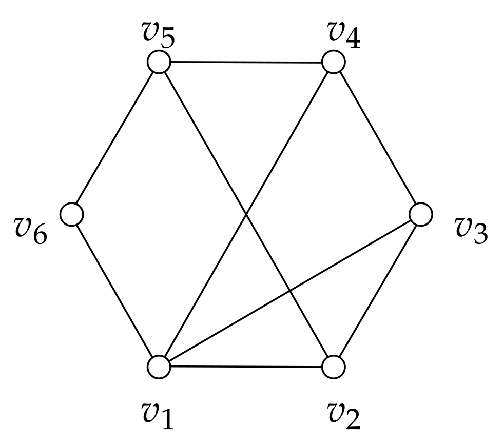
A cycle in G is a path where also . Two vertices and are consecutive in the cycle if or . A chord of a cycle is an edge joining two non-consecutive vertices in the cycle. We denote by any cycle with vertices, whereas denotes a hole, i.e., a cycle , , without chords. The chord distance of a cycle is denoted by and is defined as the minimum number of consecutive vertices in such that every chord of is incident to some of such vertices (see Figure 1 for an example of chord distance). We assume .
The length of any shortest path between two vertices x and y in a graph G is called distance and is denoted by . Moreover, the length of any longest induced path between them is denoted by . If x and y are distinct vertices, we use the symbols and to denote any shortest and any longest induced path between x and y, respectively. Sometimes, when no ambiguity occurs, we also use and to denote the sets of vertices belonging to the corresponding paths. If , then is a cycle-pair if there exist two induced paths and such that . In other words, if is a cycle-pair, then there exist induced paths and such that the vertices in form a cycle in G; this cycle is denoted by . In Figure 1 is a cycle-pair that induces the cycle ; in particular, is induced by and . We use the symbol to denote the set containing all pairs of connected vertices that induce the stretch number of G, namely . The following lemma states that cycle-pairs are useful to determine the stretch number.
Lemma 1
(from [12]). Let G be a graph such that . The following relationships hold:
- for each pair such that ,
- there exists a cycle-pair that induces the stretch number of G, that is .
This lemma suggests that studying concerns the analysis of cycles in G. In particular, if is a cycle-pair that belongs to , then the cycle is called inducing-stretch cycle for G. In Figure 1, the represented graph G belongs to ; moreover, both and are cycle-pairs in , and is the corresponding inducing-stretch cycle.
3. A Characterization Based on Forbidden Subgraphs
A well known characterization based on minimal forbidden subgraphs has been provided for the class of distance-hereditary graphs.
Theorem 2
This result can be easily reformulated, and simplified, by using the notion of chord distance. In particular, it is possible to characterize in a compact way all the forbidden subgraphs by using just the notion of chord distance as follows:
- G is a distance-hereditary graph if and only if the following graphs are not induced subgraphs of G:
- (i)
- , for each ;
- (ii)
- cycles with ;
- (iii)
- cycles with .
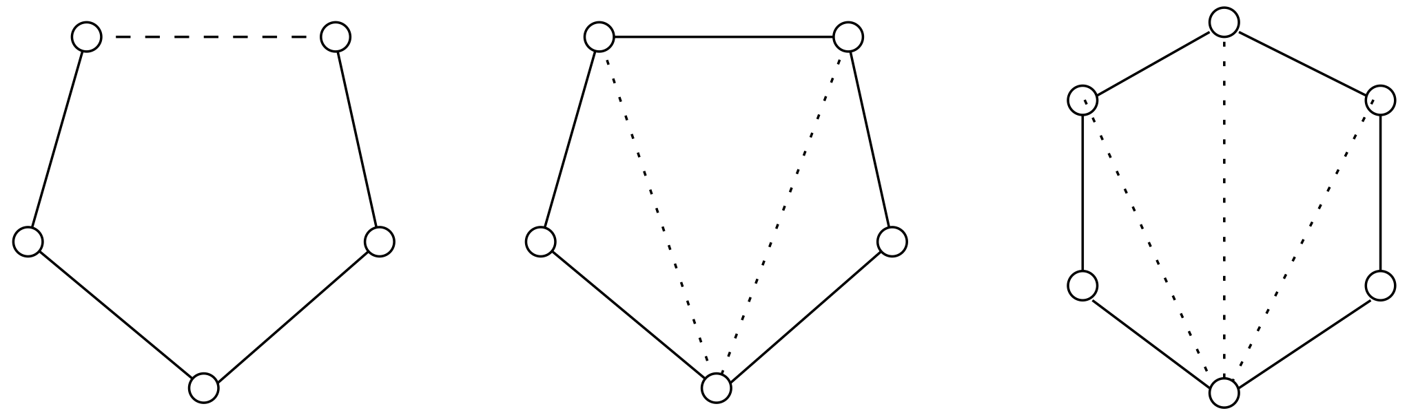
It is worth to notice that in this way we do not consider the minimal subgraphs only (cf. Figure 3).
In the following we provide a characterization similar to that of Theorem 2 for any graph . Before giving such a result, we need to recall the following technical lemma.
Lemma 2.
Let G be a graph and let be an inducing-stretch cycle of G defined by the induced paths and . If then must be incident to chords of the cycle .
Proof.
Since is an inducing-stretch cycle of G, then . If is not incident to any chords of , then the induced paths and imply , a contradiction. □
Let G be any graph. According to Lemma 1, let us consider an inducing-stretch cycle of G. Assume that is formed by the vertices of the induced paths and . Since and are induced paths, each chord of (if any) joins vertices and , with and . When some vertex is incident to chords of , we denote by and the leftmost and rightmost chords of , respectively. Formally, the indices and are defined as follows:
Theorem 3.
Let G be a graph. if and only if the following graphs are not induced subgraphs of G:
- (i)
- , for each ;
- (ii)
- cycles with ;
- (iii)
- cycles with ;
- (iv)
- cycles with .
Proof.
(⇒) Each provided hole and cycle has stretch number greater or equal to 2, and hence it cannot be an induced subgraph of G.
- (⇐)
- We prove that if , then G contains one of the subgraphs in items , , , or , or G contains a proper induced subgraph such that . In the latter case, we can recursively apply to the following proof.
According to Lemma 1, consider an inducing-stretch cycle of G and assume it is formed by the vertices of the induced paths and . Notice that, since and are induced paths, each possible chord of joins vertices and , with and .
Since by hypotheses, then by Item of Lemma 1, and hence . According to the value of q, we analyze two different cases:
- :
- In this case, if is chordless, then it corresponds to a hole as described in Item . If the chord distance of is equal to 1, all chords are incident to . According to p, we have:
- :
- corresponds to the cycle in Item ;
- :
- corresponds to the cycle in Item ;
- :
- corresponds to the cycle in Item ;
- :
- Let be the leftmost chord of . If the cycle corresponds to the cycle in Item . When , consider the subgraph induced by the vertices in the cycle . The induced paths and provide the following lower bound for :
Hence, is a proper subgraph of G with . The statement follows by recursively applying to this proof.
- :
- In this case, according to Lemma 2, must be incident to chords. We now analyze two cases with respect to the value of , being the rightmost chord of :
- :
- Consider the subgraph induced by the vertices in the cycle . In this case, the induced paths and provide the following lower bound for : . Hence, is a proper subgraph of G with . The statement follows by recursively applying to this proof.
- :
- in this case the induced paths and provide the following lower bound for :
Since is equivalent to (which holds by hypothesis), then the subgraph induced by the vertices in both and is a proper subgraph of G with stretch and . Hence, the statement follows by recursively applying to this proof.
This concludes the proof. □
4. A Characterization Based on Cycle-Chord Conditions
For the class of distance-hereditary graphs, Howorka provided the following well known characterization based on cycle-chord conditions.
Theorem 4
(from [1]). Let G be a graph. if and only if each cycle , , of G has two crossing chords.
In [12], this result has been reformulated in terms of chord distance:
Theorem 5
(from [12]). Let G be a graph. if and only if for each cycle , , of G.
In the remainder of this section, we provide a similar characterization for graphs belonging to .
Lemma 3.
Let G be a graph. If then G contains, as induced subgraph, a cycle with chord distance at most 1.
Proof.
According to Lemma 1, consider an inducing-stretch cycle of G. Since , assume that is formed by the vertices of the induced paths and , with .
If then the proof is concluded. In fact, cycle has 6 vertices and every chord of (if any) is incident to .
In the remainder of the proof assume . In this case, according to Lemma 2, is incident to chords of . Let be the rightmost chord incident to . We analyze different cases according to the value of .
- Assume . In this case, the induced paths and provide a stretch number , a contradiction.
- Assume . In this case, the induced paths and provide the following lower bound on :This contradicts .
It follows that either or . In the first case the cycle represents the requested cycle : chords of (if any) are all incident to . In the second case consider the induced paths and . These paths induce the following lower bound on :
Hence, the above paths induce a proper subgraph of G with stretch number 2. Hence, this proof can be recursively applied to . □
Lemma 4.
Let G be a graph. if and only if G contains, as an induced subgraph, a cycle , , with chord distance at most 1.
Proof.
(⇐) Trivial.
- (⇒)
- If , then it is sufficient to use Lemma 3. Now, let us assume that such that p and q are coprime. By Lemma 1, if is an inducing-stretch cycle of G, according to the hypotheses, we may assume that is formed by the vertices of the induced paths and , with .
If , then contains at least 6 vertices and all its chords (if any) are incident to . Then, corresponds to the requested cycle.
In the remainder, assume that . In this case, by Lemma 2, vertex is incident to chords of : let be the rightmost chord incident to it.
If , then the two induced paths and provide the following lower bound for :
Now we show that
It can be easily observed that Equation (1) is equivalent to
Since and by hypothesis, then Equation (2) holds. This implies that , a contradiction.
Then, it follows that . In this case, is an induced cycle with vertices and chord distance at most 1 (In C, all the possible chords are incident to ). This concludes the proof. □
This lemma can be reformulated so that it directly provides a characterization for the graphs under consideration.
Theorem 6.
Let G be a graph. if and only if for each cycle , , of G.
Compare Theorems 5 and 6 to observe the similarity between the cycle-chord characterizations of graphs with stretch number equal to 1 and graphs with stretch number less than 2, respectively.
5. Recognition Algorithm
The distance-hereditary graphs, i.e., graphs in , can be recognized in linear time [16], while the recognition problem for the generic class , k not fixed, is co-NP-complete [12]. For small and fixed values of k, in [14] a partial answer to this basic problem is given. In particular, Lemma 1 states that for , only specific rational numbers may act as stretch numbers. In [14], a characterization for each class , , has been provided, and such a characterization led to a polynomial time algorithm for the recognition problem for the class , with fixed . Unfortunately, the running time of this algorithm is bounded by .
In this section, we propose a polynomial-time algorithm for solving the recognition problem for the class according to the following approach. Lemma 4 provides a characterization for all graphs not belonging to . It is based on detecting whether a given graph G contains or not an induced cycle , , with chord distance at most 1. Now, assume that we have an algorithm returning true if and only if a given graph G contains such a cycle. Then, to recognize whether we can simply use on G and certify the membership if and only if return false. In the remainder of this section we show that such an algorithm can be defined.
5.1. An Existing Hole Detection Algorithm
We remind that denotes a hole, i.e., a chordless cycle with vertices. In [15], Nikolopoulos and Palios provided the following result about the hole detection problem.
Theorem 7
(from [15]). Given any connected graph with and , it is possible to determine whether G contains a hole in time and space.
They also extended their result to larger versions of holes.
Corollary 1
(from [15]). Let be a connected graph with and , and let be a constant. It is possible to determine whether G contains a hole on at least k vertices in time and space if , and in time and space if .
Therefore, according to this corollary, it is possible to check whether G contains a hole , with vertices, in time and space.
5.2. Quasi-Hole Detection Algorithm
We call quasi-hole any cycle such that and . In what follows, we show that the hole-detection algorithms recalled in Theorem 7 and Corollary 1 can be adapted to detect quasi-holes in any connected graph G. This adapted version is called and it is described in pseudo-code as shown in Algorithms 1 and 2. The strategy behind is based on the following result:
Lemma 5.
A connected graph G contains a quasi-hole if and only if there exists a cycle , , in G such that each path , , is a of G.
Proof.
(⇒) If G contains a quasi-hole then the vertices of form a cycle fulfilling the conditions of the statement (where is the only vertex incident to possible chords of the cycle).
- (⇐)
- Suppose that G admits cycles as described in the statement, and let be the shortest among such cycles. We now show that C has at least 5 vertices and :
- Since C fulfills the conditions of the statement, then C contains at least 5 vertices;
- Suppose by contradiction that . Then, there must exist chords with both and different from . To each chord not incident on , we associate a “length” defined as . Now, let , with , be a chord with minimum length. By definition, holds. Since is a , then , and hence results to be a cycle with at least 5 vertices. Moreover, between and , for each , , cannot exist an edge, otherwise it would be a chord with length smaller than .
Since is a cycle with at least 5 vertices and with chord distance zero, then it contradicts the fact that C is the shortest among the cycles fulfilling the conditions of the statement. Hence, .
Since both the properties at points and hold, it follows that C is a quasi-hole. □
| Algorithm 1: A quasi-hole detection algorithm. |
 |
The above lemma is used by the provided algorithm for the detection of quasi-holes in G. To this end, we associate to G a directed graph defined as follows:
- is ain the graph is the vertex set of ;
- is ain the graph is the edge set of .
If is a path of G, then both the vertices and belong to . In a similar way, if is a path of G, then the edges and must be contained in . Hence, visiting is equivalent to proceeding along s of G. It follows that the conditions of Lemma 5 on G can be verified by performing a revised DFS on (cf. [17]). In turn, the following lemma holds:
Lemma 6.
Let G be any connected graph, and let be its associated directed graph. By performing a DFS on , if the DFS-path is , where for each and for some ℓ such that , then are vertices forming a cycle in G that fulfill Lemma 5. Conversely, if G contains a quasi-hole, the DFS on will meet a sequence of vertices in whose corresponding s in G produce a path as the path in the cycle as in Lemma 5.
| Algorithm 2: A recursive procedure used by to perform an adapted DFS. |
 |
By following the same strategy used in [15], to reduce the space complexity required by , the DFS on is simulated by performing a revised DFS directly on G. This revised DFS on G is implemented by Algorithm (cf. Figure 1).
At Line 1, the algorithm computes the adjacency matrix of G from its adjacency-list (we assume that G is provided as input according to this representation). is used to check the adjacency in constant time. At Line 2, each vertex of G is checked against the following possible role: belongs to a quasi-hole C and all the chords of C, if any, are adjacent to . To perform this check, at Line 6 we consider each edge in G: if this edge, along with (cf. Line 7) or (cf. Line 12), form a path with three vertices, then the algorithm tries to extend this path into the requested cycle by recursively calling the Procedure (see Algorithm 2).
works according to Lemma 5: in any step, it attempts to extend a path defined by into s of the form ; then, for each such , the procedure proceeds by extending the formed by into s of the form , and so on. In this situation, the active-path is first extended from to , then to and so on. In case of backtracking, the last vertex is removed of the current active-path. By proceeding in this way, two cases may occur:
- the initial vertex (called in the algorithm) is added again to the active-path (cf. Line 4). If the length of the active-path is 5 or more (cf. Line 5), then the graph contains a cycle fulfilling the conditions of Lemma 5 and hence a quasi-hole is found;
- at the end of the active-path there is a vertex different from but already inserted in the active-path (cf. Lines 12–13). In this case, again the conditions of Lemma 5 apply, but now we are sure that a hole is found.
It is worth to remark that the ongoing active-path P on G and the ongoing DFS-path on contain exactly the same vertices: the elements of P correspond to the vertices of the s associated with the elements of (in P, the repeated vertices of G in adjacent s are present only once).
We now explain the role of the additional data structures and . The former is an auxiliary array of size n used to check if a vertex appears in the “active path” computed so far; given u, is equal to 1 if u appears in the active path, 0 otherwise. Concerning the latter, during the visit on , vertices that correspond to path s of G are recorded so that they are not “visited” again. The entry equals one if and only if the vertices induce as a path of G already encountered during the DFS, otherwise it equals zero. Since has entries and for each edge and for each , then its size is . Notice that registers the entry of at the beginning, thus avoiding another execution on the same path . In this way, is executed exactly once for each path of G.
Notice that the description of assures that starting from a formed by we proceed to a formed by only if is a path of G. The only exception is when coincides with the starting vertex selected at Line 2 by : in such a case may have chords from . For this purpose, the initial vertex is assigned to the variable (cf. Line 4 of the main algorithm) and it is later passed to (cf. Lines 9 and 14 of the main algorithm).
We can now provide the following statement:
Theorem 8.
Given any connected graph with and , it is possible to determine whether G contains a quasi-hole in time and space.
Proof.
According to the above description of , its correctness follows from Lemmas 5 and 6, and from the inherent execution of DFS on . In the remainder of the proof we analyze the complexity of the algorithm about the required time and space.
As G is a connected graph, we get . Concerning the data structures used by the algorithm, we assume that from any edge it is possible to access in constant time both its endpoints; alike, from any entry in the adjacency matrix of G corresponding to and it is possible to access in constant time the edge .
Consider first the time complexity of performing the revised DFS of G. The visit starts at Line 1, and proceeds by recursive calls to . This recursive procedure checks each path of G which is a and tries to extend it into a of the form . Notice that each set of vertices where is a and is adjacent to is uniquely characterized by the ordered pair where and are ordered pairs of adjacent vertices in G. Hence, the time required to perform the whole visit according to the recursive executions of is . We can now determine the time complexity of . Step at Line 1 clearly takes time. The subsequent loop at Line 2 is repeated times, and for each step the algorithm requires time for the initialization at Line 3 and, as described before, time for visiting G according to the recursive calls to .
It follows that the final time complexity is . The algorithm requires space: and for the arrays and , respectively, and for the adjacency matrix and the adjacency-list used to represent G. □
5.3. Detecting Quasi-Hole on at Least k Vertices
As in [15], the strategy described above to define a quasi-hole detection algorithm can be generalized to built algorithms for the detection of quasi-holes on at least k vertices, with . For any input graph G, we consider the following family of directed graphs :
- is an induced path in is the vertex set of ,
- is an induced path in is the edge set of .
By definition, and where is the direct graph associated to G in Section 5.2. Therefore, in the same way that running DFS on allowed us to detect quasi-holes (on at least five vertices), running DFS on allows us to detect (extended) quasi-holes on at least k vertices, for each constant . This is ensured by the following statement, which represents a generalization of Lemma 5:
Lemma 7.
Given a constant , a graph G contains a quasi-hole on at least k vertices if and only if G contains a cycle , with , such that is an induced path of G for each .
Lemmas 6 and 7 induce the following statement:
Corollary 2.
Let G be a connected graph and let be a constant. Assume that a DFS is executed on , the directed graph associated to G. If the active path computed by the DFS is , where for all , and for some p such that , then are vertices forming a cycle in G that fulfill the conditions of Lemma 7. Conversely, if G contains a quasi-hole on at least k vertices, the DFS on will meet a sequence of vertices whose associated s in G form a path as the path in the cycle of Lemma 7.
Additionally, in this situation we do not build since we implicitly run DFS on this associated graph. In particular, we process each unvisited of G as follows: we try to extend the induced path formed by into s of the form ; then, for each such , we proceed by extending the into s, and so on. Since there exist induced paths on vertices and on vertices, and it requires time to detect whether a vertex extends a into a , we have the following corollary:
Corollary 3.
Let be a connected graph with and , and let be a constant. By implicitly running DFS on it is possible to detect whether G contains a quasi-hole on at least k vertices in time when , and in time when .
The space required is when , and when . According to Lemma 4 and Corollary 3, we finally get the following result:
Theorem 9.
Let be a connected graph with and . It is possible to recognize whether in time and space.
6. Conclusions
In this paper, we studied the class . It contains each graph G with stretch number less than two, that is . These graphs form a superclass of the well studied distance-hereditary graphs, which corresponds to graphs with stretch number equal to one.
For the class we provided: (1) a characterization based on listing all the minimal forbidden subgraphs, (2) a characterization based on cycle-chord properties, and (3) a recognition algorithm that works in time and space. This algorithm exploits the result based on the cycle-chord property to detects quasi-holes in a graph; it is a simple adaptation of the algorithm provided in [15] for detecting holes.
The characterizations found seem to suggest that the graphs in and those in may be really similar in structure and hence properties. As a consequence, it would be interesting to determine whether the class can be also characterized according to generative operations (we remind that the generative properties resulted as the most fruitful for devising efficient algorithms for distance-hereditary graphs). This problem has been partially addressed in [18,19].
On the contrary, Theorem 1 could suggest that graphs with stretch number greater or equal to two may have a completely different structure with respect to those in .
Another possible extension of this work could be to investigate in the class other specific combinatorial problems that have been solved in the class of distance-hereditary graphs.
Funding
This research received no external funding.
Institutional Review Board Statement
Not applicable.
Informed Consent Statement
Not applicable.
Data Availability Statement
Not applicable.
Conflicts of Interest
The author declares no conflict of interest.
References
- Howorka, E. Distance-hereditary graphs. Q. J. Math. 1977, 28, 417–420. [Google Scholar] [CrossRef]
- Bandelt, H.J.; Mulder, H.M. Distance-hereditary graphs. J. Comb. Theory Ser. B 1986, 41, 182–208. [Google Scholar] [CrossRef] [Green Version]
- Brandstädt, A.; Le, V.B.; Spinrad, J.P. Graph Classes: A Survey; Society for Industrial and Applied Mathematics: Philadelphia, PA, USA, 1999. [Google Scholar]
- Brandstädt, A.; Dragan, F.F. A linear-time algorithm for connected r-domination and Steiner tree on distance-hereditary graphs. Networks 1998, 31, 177–182. [Google Scholar] [CrossRef]
- Chang, M.S.; Hsieh, S.Y.; Chen, G.H. Dynamic Programming on Distance-Hereditary Graphs. In International Symposium on Algorithms and Computation; Lecture Notes in Computer Science; Springer: Berlin/Heidelberg, Germany, 1997; Volume 1350, pp. 344–353. [Google Scholar]
- Gioan, E.; Paul, C. Dynamic distance hereditary graphs using split decomposition. In International Symposium on Algorithms and Computation; Lecture Notes in Computer Science; Springer: Berlin/Heidelberg, Germany, 2007; Volume 4835, pp. 41–51. [Google Scholar]
- Lin, C.; Ku, K.; Hsu, C. Paired-Domination Problem on Distance-Hereditary Graphs. Algorithmica 2020, 82, 2809–2840. [Google Scholar] [CrossRef]
- Nicolai, F.; Szymczak, T. Homogeneous sets and domination: A linear time algorithm for distance-hereditary graphs. Networks 2001, 37, 117–128. [Google Scholar] [CrossRef]
- Rao, M. Clique-width of graphs defined by one-vertex extensions. Discret. Math. 2008, 308, 6157–6165. [Google Scholar] [CrossRef]
- Cicerone, S.; Di Stefano, G.; Flammini, M. Compact-Port Routing Models and Applications to Distance-Hereditary Graphs. J. Parallel Distrib. Comput. 2001, 61, 1472–1488. [Google Scholar] [CrossRef] [Green Version]
- Esfahanian, A.H.; Oellermann, O.R. Distance-hereditary graphs and multidestination message-routing in multicomputers. J. Comb. Math. Comb. Comput. 1993, 13, 213–222. [Google Scholar]
- Cicerone, S.; Di Stefano, G. Graphs with bounded induced distance. Discret. Appl. Math. 2001, 108, 3–21. [Google Scholar] [CrossRef] [Green Version]
- Cicerone, S. Characterizations of Graphs with Stretch Number less than 2. Electron. Notes Discret. Math. 2011, 37, 375–380. [Google Scholar] [CrossRef]
- Cicerone, S.; Di Stefano, G. Networks with small stretch number. J. Discret. Algorithms 2004, 2, 383–405. [Google Scholar] [CrossRef]
- Nikolopoulos, S.D.; Palios, L. Detecting Holes and Antiholes in Graphs. Algorithmica 2007, 47, 119–138. [Google Scholar] [CrossRef] [Green Version]
- Hammer, P.L.; Maffray, F. Completely separable graphs. Discret. Appl. Math. 1990, 27, 85–99. [Google Scholar] [CrossRef] [Green Version]
- Cormen, T.H.; Leiserson, C.E.; Rivest, R.L.; Stein, C. Introduction to Algorithms, 2nd ed.; The MIT Press and McGraw-Hill Book Company: New York, NY, USA, 2001. [Google Scholar]
- Cicerone, S. Using Split Composition to Extend Distance-Hereditary Graphs in a Generative Way—(Extended Abstract). In International Conference on Theory and Applications of Models of Computation; Lecture Notes in Computer Science; Springer: Berlin/Heidelberg, Germany, 2011; Volume 6648, pp. 286–297. [Google Scholar] [CrossRef]
- Cicerone, S. On Building Networks with Limited Stretch Factor. In Web, Artificial Intelligence and Network Applications, Proceedings of the Workshops of the 34th International Conference on Advanced Information Networking and Applications, AINA, Caserta, Italy, 15–17 Aprli 2020; Advances in Intelligent Systems and Computing; Springer: Berlin/Heidelberg, Germany, 2020; Volume 1150, pp. 926–936. [Google Scholar] [CrossRef]
Figure 1.
The chord distance of this graph is two because: (i) vertices and are consecutive in the cycle, (ii) every chord is incident to one of such vertices, and (iii) there is no other set with less than two vertices with the same properties.
Figure 1.
The chord distance of this graph is two because: (i) vertices and are consecutive in the cycle, (ii) every chord is incident to one of such vertices, and (iii) there is no other set with less than two vertices with the same properties.

Figure 2.
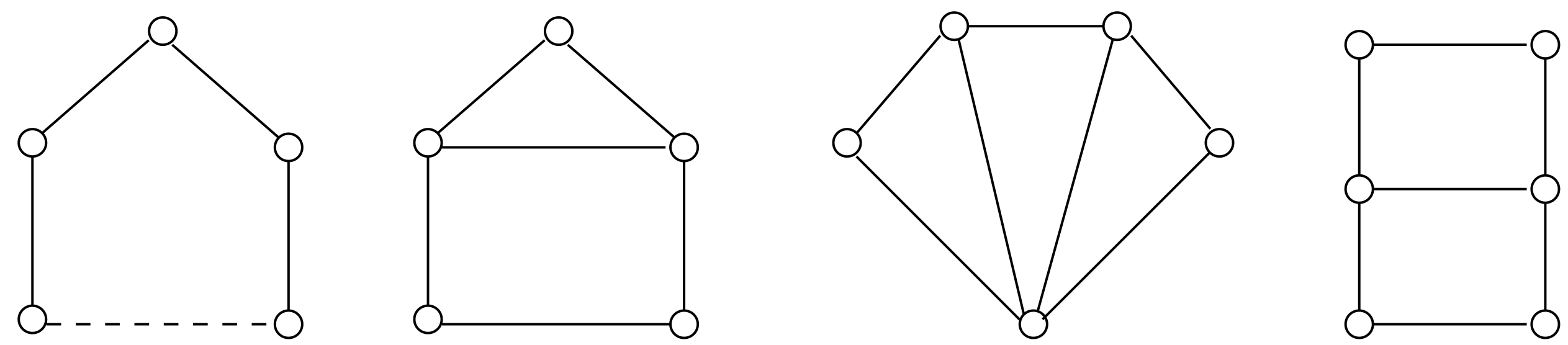
The minimal forbidden subgraphs of distance-hereditary graphs: from left to right, the hole, the house, the fan, and the domino. Dashed lines represent paths of length at least one.
Figure 2.
The minimal forbidden subgraphs of distance-hereditary graphs: from left to right, the hole, the house, the fan, and the domino. Dashed lines represent paths of length at least one.

Figure 3.
The forbidden subgraphs of expressed according to the notion of chord distance. Dashed lines represent paths of length at least one. Dotted lines represent chords that may or may not exist.
Figure 3.
The forbidden subgraphs of expressed according to the notion of chord distance. Dashed lines represent paths of length at least one. Dotted lines represent chords that may or may not exist.

Figure 4.
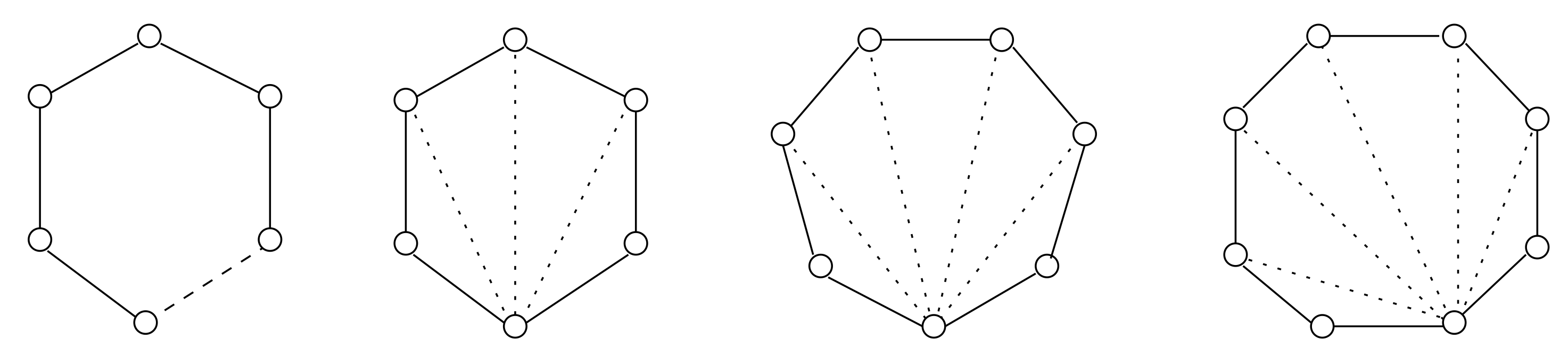
The forbidden subgraphs of graphs having stretch number less than 2. Dashed (dotted, respectively) lines represent paths of length at least one (chords that may or may not exist, respectively).
Figure 4.
The forbidden subgraphs of graphs having stretch number less than 2. Dashed (dotted, respectively) lines represent paths of length at least one (chords that may or may not exist, respectively).

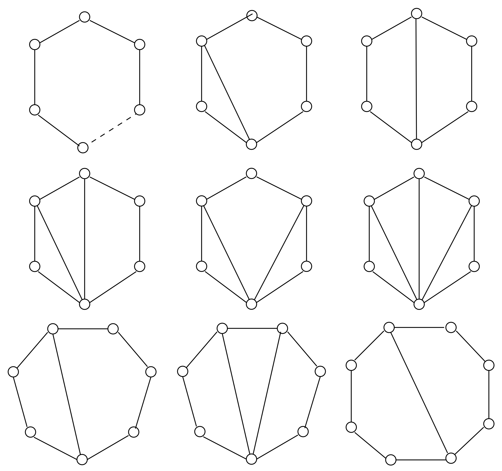
Figure 5.
The minimal forbidden subgraphs of any graph with stretch number less than 2. Dashed lines represent paths of length at least one.
Figure 5.
The minimal forbidden subgraphs of any graph with stretch number less than 2. Dashed lines represent paths of length at least one.

Publisher’s Note: MDPI stays neutral with regard to jurisdictional claims in published maps and institutional affiliations. |
© 2021 by the author. Licensee MDPI, Basel, Switzerland. This article is an open access article distributed under the terms and conditions of the Creative Commons Attribution (CC BY) license (http://creativecommons.org/licenses/by/4.0/).
Share and Cite
MDPI and ACS Style
Cicerone, S. A Quasi-Hole Detection Algorithm for Recognizing k-Distance-Hereditary Graphs, with k < 2. Algorithms 2021, 14, 105. https://0-doi-org.brum.beds.ac.uk/10.3390/a14040105
AMA Style
Cicerone S. A Quasi-Hole Detection Algorithm for Recognizing k-Distance-Hereditary Graphs, with k < 2. Algorithms. 2021; 14(4):105. https://0-doi-org.brum.beds.ac.uk/10.3390/a14040105
Chicago/Turabian StyleCicerone, Serafino. 2021. "A Quasi-Hole Detection Algorithm for Recognizing k-Distance-Hereditary Graphs, with k < 2" Algorithms 14, no. 4: 105. https://0-doi-org.brum.beds.ac.uk/10.3390/a14040105
Note that from the first issue of 2016, this journal uses article numbers instead of page numbers. See further details here.