
Optimization of the Multi-Facility Location Problem Using Widely Available Office Software


1
Department of Logistics, University of Defence, Kounicova 65, 662 10 Brno, Czech Republic
2
Department of Intelligence Support, University of Defence, Kounicova 65, 662 10 Brno, Czech Republic
*
Author to whom correspondence should be addressed.
Algorithms 2021, 14(4), 106; https://0-doi-org.brum.beds.ac.uk/10.3390/a14040106
Submission received: 18 February 2021
/
Revised: 23 March 2021
/
Accepted: 24 March 2021
/
Published: 26 March 2021
(This article belongs to the Special Issue Network Science: Algorithms and Applications)
Abstract
:Multi-facility location problem is a type of task often solved (not only) in logistics. It consists in finding the optimal location of the required number of centers for a given number of points. One of the possible solutions is to use the principle of the genetic algorithm. The Solver add-in, which uses the evolutionary method, is available in the Excel office software. It was used to solve the benchmark in 4 levels of difficulty (from 5 centers for 25 points to 20 centers for 100 points), and one task from practice. The obtained results were compared with the results obtained by the metaheuristic simulated annealing method. It was found that the results obtained by the evolutionary method are sufficiently accurate. Their accuracy depends on the complexity of the task and the performance of the HW used. The advantage of the proposed solution is easy availability and minimal requirements for user knowledge.
1. Introduction
In this work we deal with the problem of finding the coordinates of c centers for b points. A typical example is finding the optimal location for c central warehouses that will serve b branches. In the literature, this problem is called the multi-facility location problem (MFLP) and there are a number of ways to solve this type of task. This problem is often solved in the field of logistics, but there are also other applications.
The article is organized into five sections. In this introduction, our motivation and the objectives of this article are presented. The first section also covers the problem formulation and the literature review. Section 2 presents the details concerning the approach and methods used. Section 3 shows the results of the experiments. Section 4 follows with the discussion about the results achieved. Finally, Section 5 concludes the article.
1.1. Literature Review
Various methods for solving facility or multi-facility location problem are described in the literature.
1.1.1. Facility Location Problems Solved in Excel Environment
Ref. [1] describes an Excel-based Decision Support System for Facility Location Problems. The aim is to select a subset of locations from a set of candidate locations, and to determine which customer locations will be served by which facility, to optimize an objective function that is based on the distances (or the costs) between the facilities and the demands of customer locations they serve.
Use of Solver Add-in in logistics is presented in [2]. The aim of the paper is to present a solution of facility location problem using the Solver add-in in Excel. In the case study discussed in the paper, the company’s central warehouse location was selected based on the classic location theory, which addresses the need to minimize the cost of transport. The mathematical model of the exercise is based on the Euclidean coordinates metrics.
Article [3] concentrates on facility location problem, focusing on the linear programming model and a genetic algorithm in the location problem analysis and analytical method. In the linear programming model, because the given complex table calculation method is too complicated and the workload is very large, the Excel software is proposed to solve the location problem, which can greatly improve the efficiency of enterprise facility location problem. In addition, a genetic algorithm based on MATLAB toolbox is applied to another type of facility location problem, which provides a referential method for location decision under different conditions and different facilities.
1.1.2. In the Area of the Rectangular Distance Multi-Facility Location Problem
A nonlinear approximation method was developed by in [4], where any number of linear and (or) nonlinear constraints defining a convex feasible region can be included.
Ref. [5] presents a new method that, as it states, efficiently handles the rectilinear distance problem MFLP having large clusters, i.e., where several new facilities are located together at one point. This paper states and proves a new necessary and sufficient optimality condition. This condition transforms the problem of computing a descent direction into a constrained linear least-squares problem. The latter problem is solved by a relaxation method that takes advantage of its special structure. The new technique is incorporated into the direct search method.
Ref. [6] develops a dual problem for the constrained multi-facility minimum location problems involving mixed norms. General optimality conditions were obtained providing new algorithms which are decomposition methods based on the concept of partial inverse of a multifunction.
As an alternative to linear programming, coordinate descent was presented in [7] as a simple approach which sometimes finds optimal locations. By deleting the term that shows the relationship between new facilities in objective function, the problem is converted to some single facility location problems to which we can apply median conditions. The first coordinate we choose is the first variable and the second coordinate is the second variable, and so on. It is continued until we obtain the same vector by coordinate descent that we have obtained previously by coordinate descent, at which point we stop.
1.1.3. In the Area of the Euclidean Multi-Facility Location Problem
In [8], the authors proposed a pseudo-gradient technique that classifies the new facilities into distinct categories based on their coincidence with other facilities in order to derive a descent method for solving Euclidean MFLP.
Author in [9] also approached Euclidean MFLP by using a general e-subgradient method in which search directions are generated based on the subdifferential of the objective function over a neighborhood of the current iterate.
In [10] developed an algorithm which, from any initial point, generates a sequence of points that converges to the closed convex set of optimal solutions to the problem Euclidean MFLP.
For the multi-facility location problem with no constraints on the location of the new facilities, authors in [11] derived some sufficient conditions for the coincidence of facilities that are valid in a general symmetric metric.
Xue et al. [12] suggested the use of polynomial-time interior point algorithm to solve the MFLP problem. They presented a procedure in which an approximate optimum to Euclidean MFLP can be recovered by solving a sequence of linear equations, each associated with an iterate of the interior point algorithm used to solve the dual problem.
1.1.4. In the Area of the Rectangular Distance Minimax Location Problem
Morris [13] introduced this problem with linear constraints which (a) limit the new facilities location and (b) enforce upper bounds on the distances between new and existing facilities and between new facilities. He used dual variables that provide information about the complete range of new facility locations which satisfies the MiniMax criterion.
Authors in [14] presented a method involving the numerical integration of ordinary differential equations and was computationally superior to methods using nonlinear programming.
1.1.5. Solutions for Other Models
A specialized simplex-based algorithm was derived in [15] for solving rectangular multiproduct MFLP.
Authors in [16] presented an iterative solution for MFLP on sphere. The procedure involved the approximation of the domain of objective function which in the limit approaches to that of the original objective function. In [17], authors considered Euclidean, squared Euclidean and the great circle distances. They formulated an algorithm and investigated its convergence properties.
1.1.6. Some Heuristic and Metaheuristic Methods
Authors [18] introduced a simple heuristic for solving MFLP with Euclidean distance. This procedure locates each of the new facilities in a temporary location at each step and locates the next new facility according to the facilities located so far. After all n new facilities are located in this manner the process is repeated and the readjustment process is continued until no further movements occur during a complete round of adjustment evaluations.
In [19] solved the MFLP with ant-colony optimization metaheuristic when the distances are rectangular and Euclidean. This algorithm produces optimal solutions for problem instances of up to 20 new facilities.
1.1.7. Solutions Using Genetic Algorithm
In the study “A Novel Nondominated Sorting Simplified Swarm Optimization for Multi-Stage Capacitated Facility Location Problems (CFLP) with Multiple Quantitative and Qualitative Objectives,” [20], a novel solution based on simplified swarm optimization (SSO) and a nondominated sorting technique is proposed to provide Pareto-optimal solutions for enhancing search efficiency and solution quality. To yield feasible solutions, three repairer mechanisms, namely, random repair, cost-based, and utility-based mechanisms, are proposed to enhance the search efficiency and diversity of each population. A fuzzy analytic hierarchy process is used to calculate the weight of qualitative objectives. To evaluate the efficiency and effectiveness of the proposed algorithm, extensive experiments are conducted on benchmark and newly generated instances of the four stages of CFLPs. Then, results are compared with those of the nondominated sorting genetic algorithm-II, multi-objective SSO, and multi-objective particle swarm optimization reported from the literature. The computational results demonstrate that the proposed algorithm is highly competitive and performs well in terms of solution quality and computational time. The Pareto set in the investigated type of facility location problems leads to solutions that may better support decision-making.
In article [21], a multi-objective multi-facility model of green closed-loop supply chain under uncertain environment is presented. In this model, the proposed green closed-loop supply chain considers three classes in the case of the leading chain and three classes in terms of the recursive chain.
In the study “A Hybrid Genetic Algorithm for Multi-emergency Medical Service Center Location-allocation Problem in Disaster Response” [22], the final patient mortality risk value (injury severity) caused by both initial mortality risk value and travel distance (travel time) is considered to determine the location-allocation of temporary emergency medical service centers.
According to the article “Multi-facilities Location and Allocation Problem of Three-Echelon Supply Chain Based on an Improved Genetic Algorithm” [23], a new mathematics model on multi-facilities location and allocation problem (MLAP) of three-echelon supply chain was built, which mainly took some logistics cost such as inventory cost, carrying cost, transportation cost into consideration. Then, an improved Genetic Algorithm was proposed to solve the MLAP. In this algorithm, the real encoding method was used to encode the solution directly, and meanwhile the crossover and mutation operator were improved. Finally, a numerical experiment showed clearly the feasibility of the IGA method and the effectiveness of the model.
In [24] the multi-objective facility layout problem is defined in the literature as an extension of the famous quadratic assignment problem (QAP). Most previous mathematical models tried to combine both the quantitative and the qualitative objectives into a single objective by using weighting factors. This paper introduces a multi-objective mathematical model and solves it using the revised Strength Pareto Evolutionary Algorithm. The purpose of work is to find an efficient set of solutions “Pareto optimal set” which could be introduced to the decision maker to select the best alternative, while considering conflicting and non-commensurate objectives. A computer program is developed to define the mathematical model, code candidate solutions into genetic form, and use Evolutionary Multi-Objective Optimization algorithms to find the efficient set of solutions.
1.1.8. Applications
The MFLP and related problems have a broad range of applications in various domains such as logistics, transportation, planning and scheduling, supply chains and many others. Foltin et al. [25] show future logistics applications in the military; they discuss the planning process and its subsequent implementation to ensure logistical support to deployed units and propose discrete event simulation for professional training.
Another example where the MFLP is used is the Tactical Decision Support System (TDSS). This system was developed to support commanders in their decision-making processes [26]. This system is composed of a number of models of military tactics for optimization of the operation task at hand, see, e.g., [27,28,29,30,31,32].
From the above, it is clear that the authors use complex proprietary methods and software to solve the problem, which are complicated and inaccessible for the ordinary manager.
1.2. Main Aim of this Work
The article discusses the possibility of using the commercial software Excel for solving MFLP and describes the problems associated with it. Plane coordinates and calculation of distances in Euclidean space are used in the calculations. The calculated data must therefore be considered approximate, serving mainly as a basis for further decisions.
In order to verify its applicability, we solve five MFLP benchmark tasks with different levels of difficulty. The benchmark tasks are designed so that it is possible to calculate the optimal solution (with the exception of the last task, which is created based on a real-world problem). We then compare the optimal solution with the result obtained by calculation in the Excel application environment and calculation by the metaheuristic method (Simulated Annealing). The tasks are solved on two computers with different performance parameters in order to verify the influence of the hardware configuration on the accuracy of the calculation. Both methods are also used to solve a practical example based on real data.
Excel software and its Solver add-in are commercial products. This work does not examine the algorithms they use. From the point of view of this research, it is a “black box” for which the inputs, settings of basic parameters and outputs are known.
The proposed procedure uses available commercial software (Excel) for solving Multi-facility location problem, as it is described in Section 1.3. This solution has not yet been described in the scientific literature. The use of the proposed procedure will allow the required calculations to be performed on a personal computer with commonly available office software. No special competencies are required; user-level knowledge is sufficient. The aim of this work is to verify the proposed procedure on test examples and to find the problems that this simplified approach brings.
1.3. Problem Formulation
The aim is to find a solution to the following problem. There are b points where the coordinates of their positions are known. There is a requirement to find the coordinates of the positions of the c centers. Each point will be assigned to exactly one center which is closest to it. Variable c is an integer greater than or equal to 1 and b is an integer greater than or equal to c.
The objective is to find the positions of the centers so that the sum of the distances between all the centers and their assigned points will be minimal.
A practical example is a company with a number of existing branches which needs to set up a number of centers that will provide services to these branches. The locations of the branches are known; the centers will be built as new. The location of these centers and the branches they will serve are not specified.
The mathematical formulation of this problem is as follows. Let be a set of points (); the coordinates of these points are known. Let be a set of centers (; the coordinates of these points are not known as they are the subject of the optimization.
The Euclidean distance between a center and any point in two-dimensional space is calculated according to Formula (1). In general, any space, number of dimensions and distance function can be used.
where is the distance between center and point
; ,
are coordinates of the center
, and
, are coordinates of point
.
The objective function of the MFLP problem is shown in Formula (2). It corresponds to the sum of distances between all points and their assigned centers which are closest to them.
The optimization goal is in Formula (3); the aim is to find the locations of c centers so that the objective function D is minimal. In the case of two-dimensional space, there are 2c continuous optimization variables.
2. Materials and Methods
2.1. Hardware and Software Configurations
Hardware configurations. Calculations were performed on two personal computers with different hardware configurations:
- PC 1-Processor: AMD A10-9620P RADEON R5, 10 COMPUTE CORES 4C + 6G 2.50 GHz. Installed memory 8.00 GB RAM.
- PC 2-Processor: INTEL CORE i7-7700 3.60 GHz. Installed memory 32.00 GB RAM.
Software configuration. System type 64-bit operating system, Windows 10 Enterprise LSTC, MS Excel 2016, 64 bit, part of the Microsoft Office Suite, with the Solver add-in installed, which performs calculations. In the basic version it allows only one method of calculation using genetic algorithms. The Excel environment is used to enter data, calculate intermediate results, and display the result of the entire process.
2.2. Benchmark Instances
To verify the applicability of the proposed solution, both from the accuracy and optimization time points of view, five benchmark instances differing in difficulty are proposed.
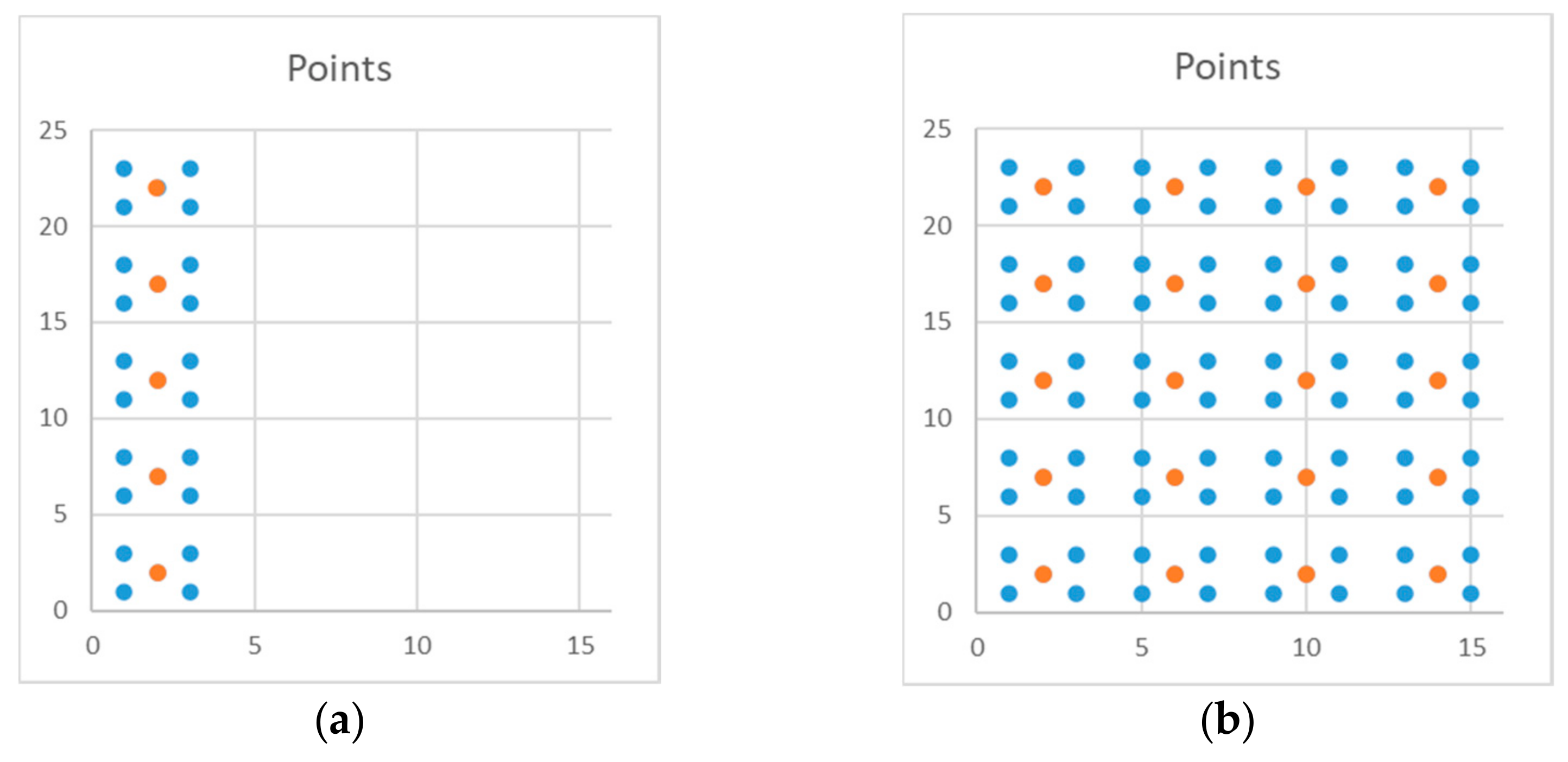
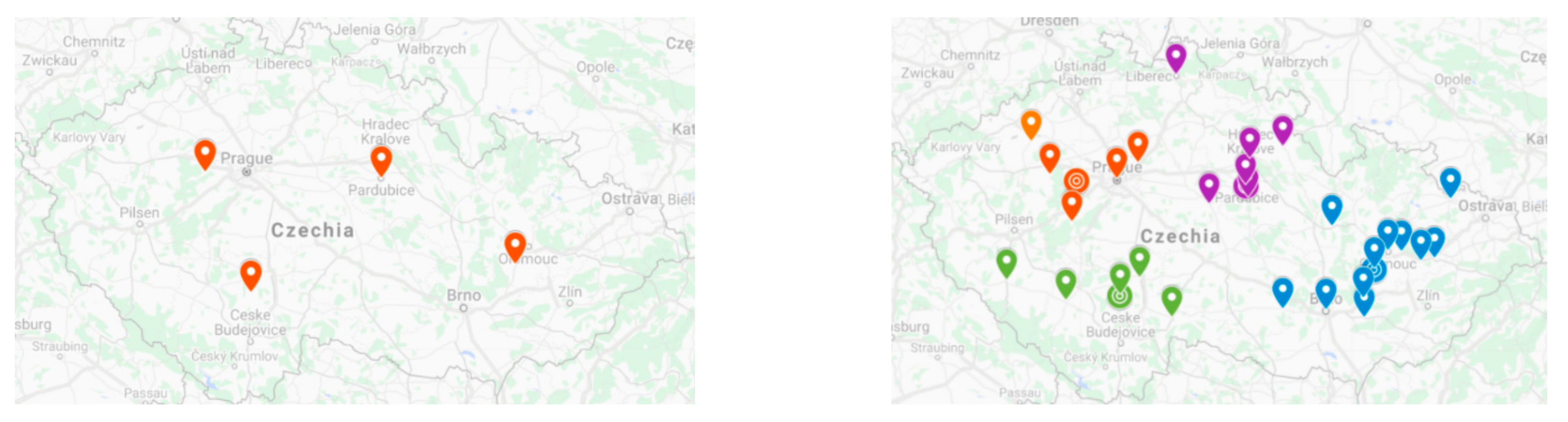
The first four instances (labeled A, B, C, D) are designed in such a way that the optimal solution can be easily determined. The points in these instances are arranged in groups of five, four at the vertices of the square, the fifth at its center. For each group, a center exists. The optimal position of the center for such a group is identical with the position of the fifth point in the center of the square. Instances A and D are shown in Figure 1 for illustration of the principle; blue circles represent points; orange circles represent centers in their optimal position. The fifth blue point in the center is covered by an orange circle.
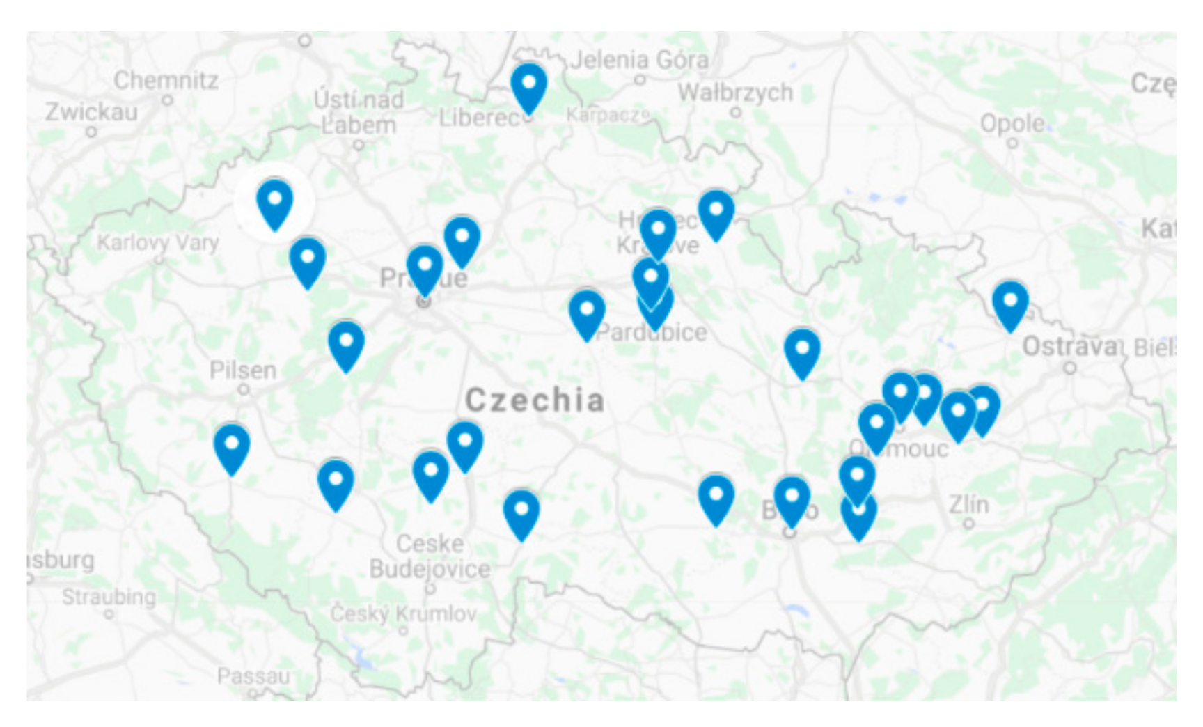
The last instance (labeled E) is created based on a real-world problem using real geographic data. There are 27 points and 4 centers to deploy. The coordinates of points are recorded in Table 1 and their visualization is shown in Figure 2. In contrast to benchmark tasks, for which it is possible to manually calculate the optimal position of the centers thanks to artificially designed points, for this type of task the optimal solution cannot be calculated in advance.
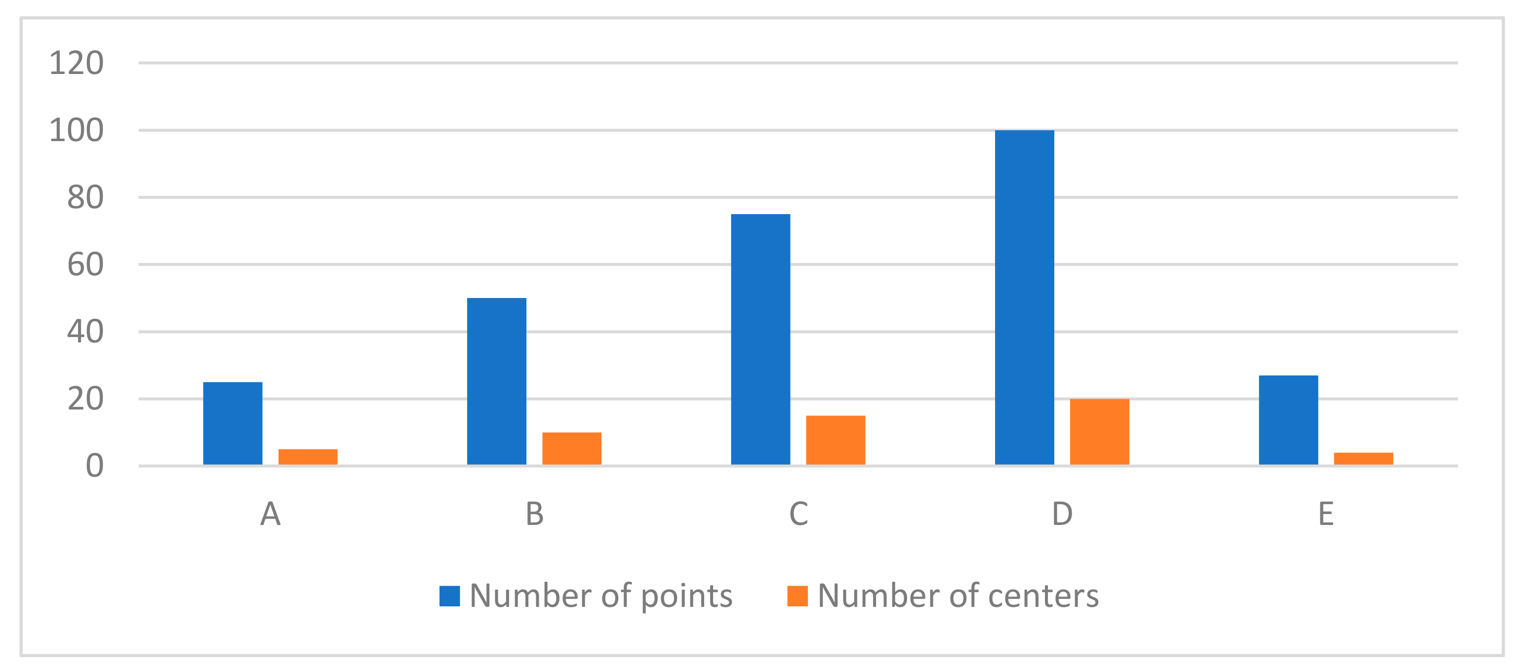
The basic parameters and the optimal solution (if available) of all the benchmark instances are shown in Table 2 and in Figure 3.
For each benchmark task, 100 optimizations were performed both in the Excel-Solver software as well as using the metaheuristic algorithm (see Section 2.4) and thus, 100 different solutions are obtained.
Each task was solved in 4 ways:
- by Excel-Solver evolutionary method on PC1;
- by Excel-Solver evolutionary method on PC2;
- by metaheuristic algorithm on PC1;
- by metaheuristic algorithm on PC2.
For each task, method and hardware configuration, the following parameters and outputs calculated from all individual solutions are recorded:
- minimal solution;
- average solution;
- standard deviation;
- difference between the optimal and the minimal solutions in percent;
- difference between the optimal and the average solutions in percent;
- histogram, classes are from 1 percent to 10 percent deviation;
- graph with coordinates for result for the minimal solution.
2.3. Evolutionary Method
This method is used for computing in Excel software with the Solver add-in. In the available help and information from the manufacturer, the method is noted as evolutionary method, with the explanation that it is used to solve non-smooth problems. Convergence values, mutation frequency, base file size, random number, and maximum time without enhancement can also be set for this method. What the effect is of changes in these parameters on the calculation is not stated; therefore, default values were left for all calculations. Default values of parameters are listed in Table 3.
2.4. Metaheuristic Algorithm
The metaheuristic algorithm used to complement the Excel Solver is based on the Simulated Annealing (SA) principle adapted for the MFLP problem. This choice was based on the previous experiences of the authors as this algorithm proved to be very successful in other position optimization problems (see [23] for more details). The principle is inspired by annealing in metallurgy, where this process is used to reduce the defects of material by way of heating and controlled cooling.
Algorithm 1 presents this method in pseudocode. The inputs of the algorithm are as follows:
- : number of centers to deploy.
- : number of points.
- : set of points.
The outputs are as follows:
- : best solution (i.e., locations of centers) found during optimization.
- : evaluation of the best solution found during optimization (objective function).
Settings of the algorithm:
- : maximum temperature (the initial value used in the first generation).
- : the threshold value of the temperature (used in the termination condition).
- : coefficient controlling the speed of temperature cooling.
- : maximum number of transformations per iteration.
- : maximum number of replacements per iteration.
Other symbols used:
- : current solution.
- : value of the current solution.
- : transformed solution.
- : value of the transformed solution.
- : probability that the transformed solution replaces the original.
- : current number of transformations in an iteration.
- : current number of replacements in an iteration.
| Algorithm 1 SA algorithm for the MFLP. |
| 1: Algorithm_MFLP_SA (,,,,,,,) 2: Generate_Random_Solution() 3: 4: 5: while do // Iterations 6: 7: while and do // Transformations 8: Transform_Solution (,,,) 9: 10: 11: with probability do // Replacements 12: 13: 14: 15: if then do 16: 17: 18: 19: 20: return , |
At the beginning (point 1), the initial deployment of centers is generated using the random number generator with uniform distribution. The value of every variable is generated in range limited by the minimum and maximum value of all the points in the corresponding axes x or y. In point 2, this solution is evaluated using the objective function in Formula (2).
The algorithm works in iterations. During an iteration (points 4 to 18), the value of temperature T is constant. In each iteration, a number of transformations of the current solution into solution is performed (see point 7). This transformed solution replaces the original (points 10 to 13) with some probability given by the Metropolis criterion (4). A better solution is always replaced. However, the key is accepting even worse solutions, thus expanding the search space explored for the global optimum. In such cases, the probability depends on the difference between both solutions and the current temperature; the smaller the difference and the bigger the temperature, the bigger the probability. An iteration is terminated (point 6) when the maximum number of transformations or replacements is performed.
The transformation of a current solution is a simple process. One variable (i.e., x or y coordinate of one of the centers) is randomly selected. Then this variable is changed using the Formula (5). The size of the change depends on the current temperature; the bigger the temperature, the bigger the change. This causes the wide exploration of the state space at the beginning of the optimization and the refinement of the solution towards the end.
where is the variable selected to be changed in solution ; is the changed variable in transformed solution ; is a random number generator with normal distribution with mean and standard deviation ; is the maximum range in which the variable can change given by the minimum and maximum coordinates in the corresponding axis x or y.
The algorithm is terminated (point 4) when the current temperature decreases below the lower threshold . The best solution found during the process is stored (see points 14 to 16) and returned at the end of the algorithm (point 19).
3. Results
In this section, results obtained by the benchmark calculations are analyzed. For a better understanding, the terms and abbreviations used are explained in Table 4 and Table 5. Table 6, Table 7, Table 8 and Table 9 are four tables of the results of the calculations of benchmark instances A, B, C, D obtained by evolutionary and metaheuristic methods on PC1 and PC2. The results are also presented in the form of histograms and graphs (Section 3.1). The best solution for benchmark E is recorded in Section 3.2.
3.1. Histograms and Solutions for Benchmark D
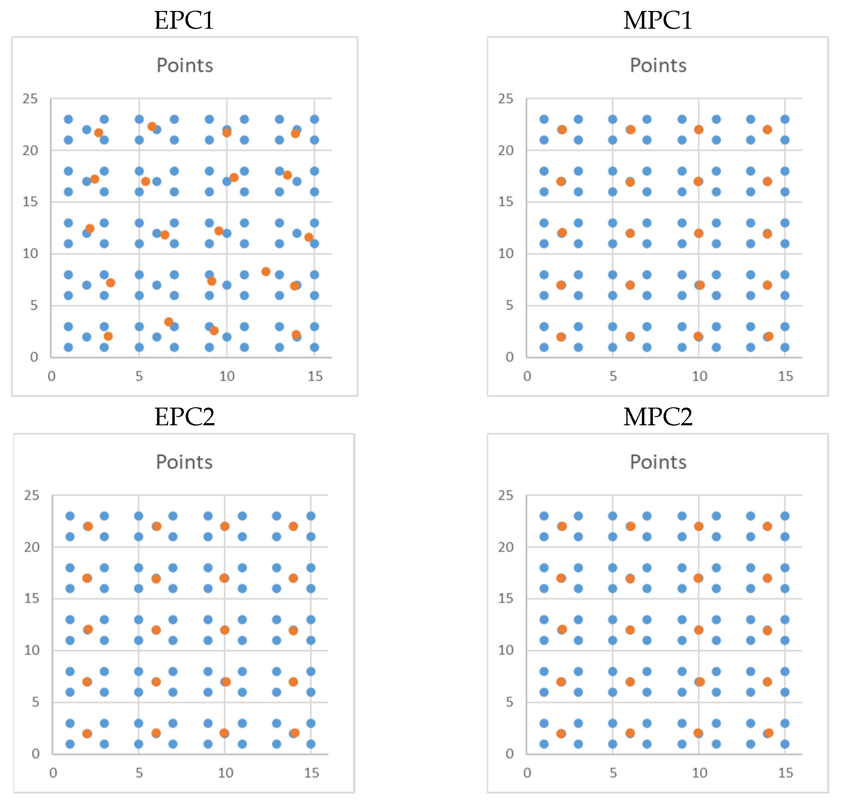
Histograms (Figure 4) and graphs with the best solution (Figure 5) are presented in this section only for benchmark instance D (20 centers for 100 points), because for this most difficult benchmark the illustration of the differences in the methods and hardware used is most obvious.
In each method 100 different results were obtained for this benchmark; they can be statistically evaluated using a histogram. The intervals are designed in the range of 101, 102 … 110 percent of the optimal value. The histogram shows the frequency of occurrence of the obtained values in a given interval. From the graph it is possible to assess how accurate the method is. For the metaheuristic method on PC1 and PC2, the histograms are the same.
3.2. Best Solution for Benchmark E
4. Discussion
This work is focused on verifying the possibility of using Excel to solve MFLP-type tasks. The quality of the result depends on the HW used and the complexity of the task. Because the software works with the generated random number during the calculations, 100 calculations were performed for each of the variants, in order to partially eliminate this fact.
The results obtained using the metaheuristic algorithm are balanced in all benchmarks on both PCs; deviations from the optimal value are in the order of hundredths of percent. Thus, the method is verified and considered suitable for obtaining the reference value of the result in the case of benchmark E.
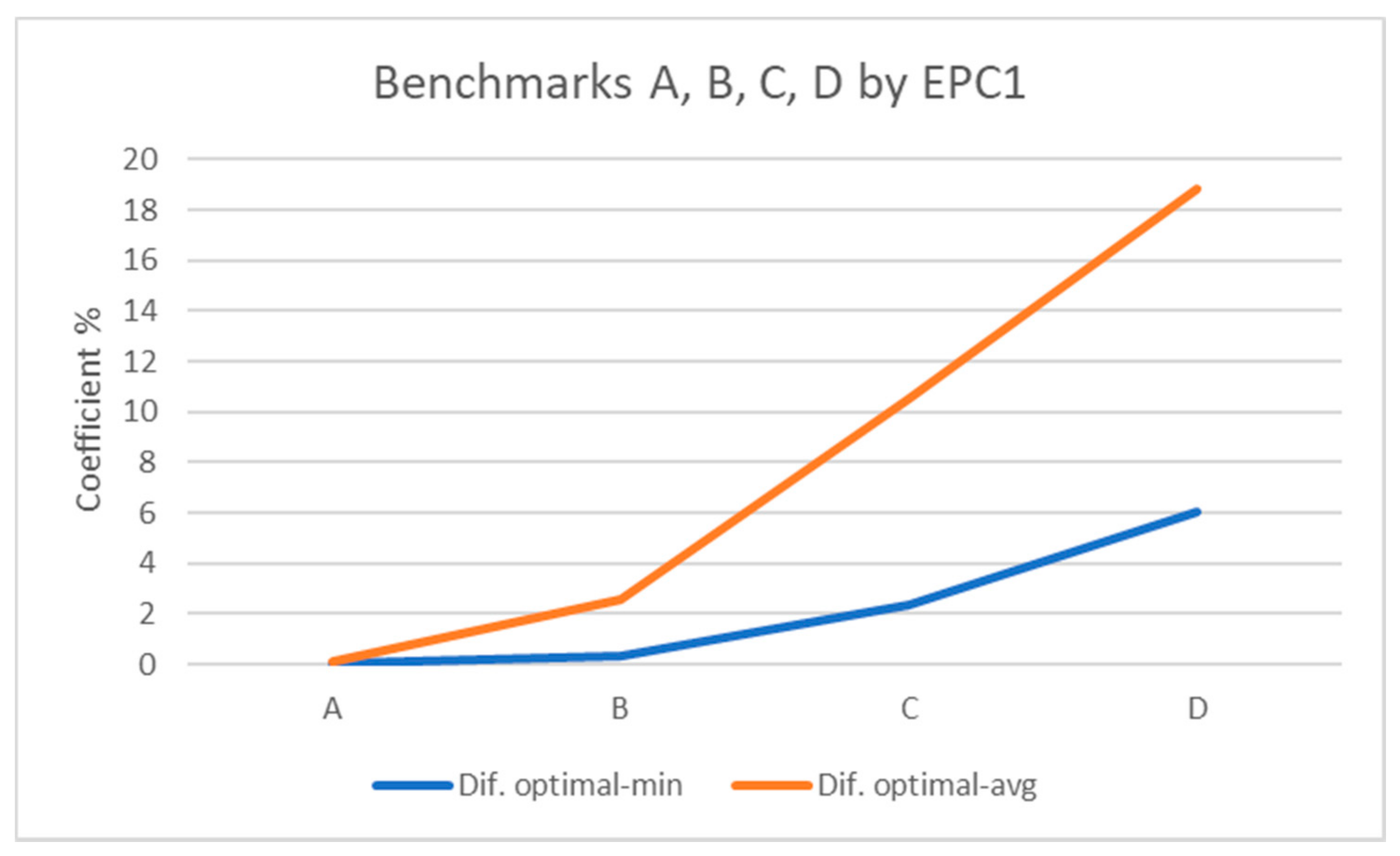
When using the evolutionary method, the influence of the complexity of the benchmark and the HW used is obvious. The EPC1 graph (Figure 7) compares two coefficients (Dif. optimal-min, Dif. optimal-avg—see Table 4), on which it is possible to present an influence of the complexity. Both values increase with the benchmark complexity. From the higher growth of the value of Dif. optimal-avg it can be concluded that for this type of task it is important to conduct more calculations and select the best; the value of Dif. optimal-min increases less. Thus, more calculations may partially eliminate inaccuracy.
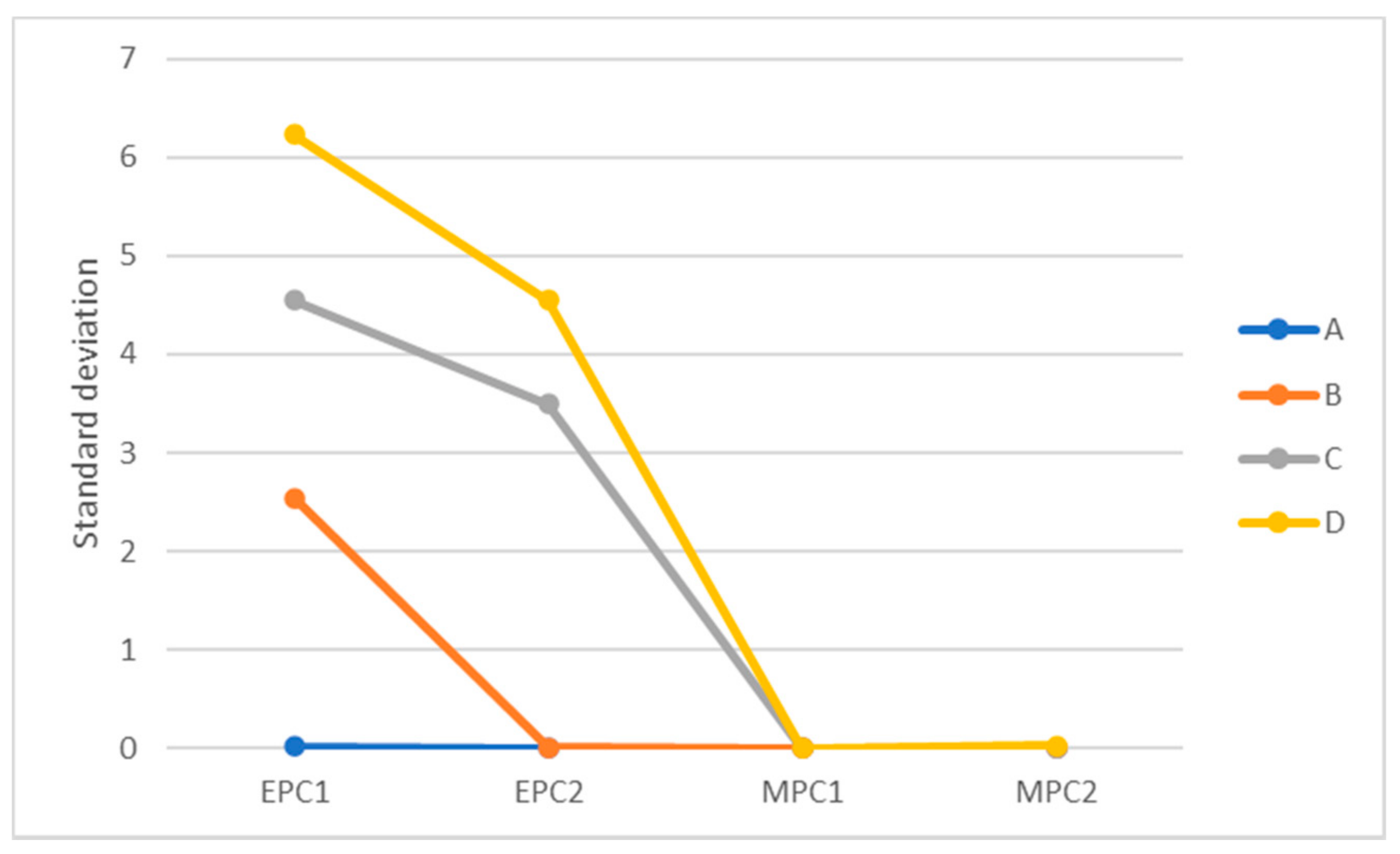
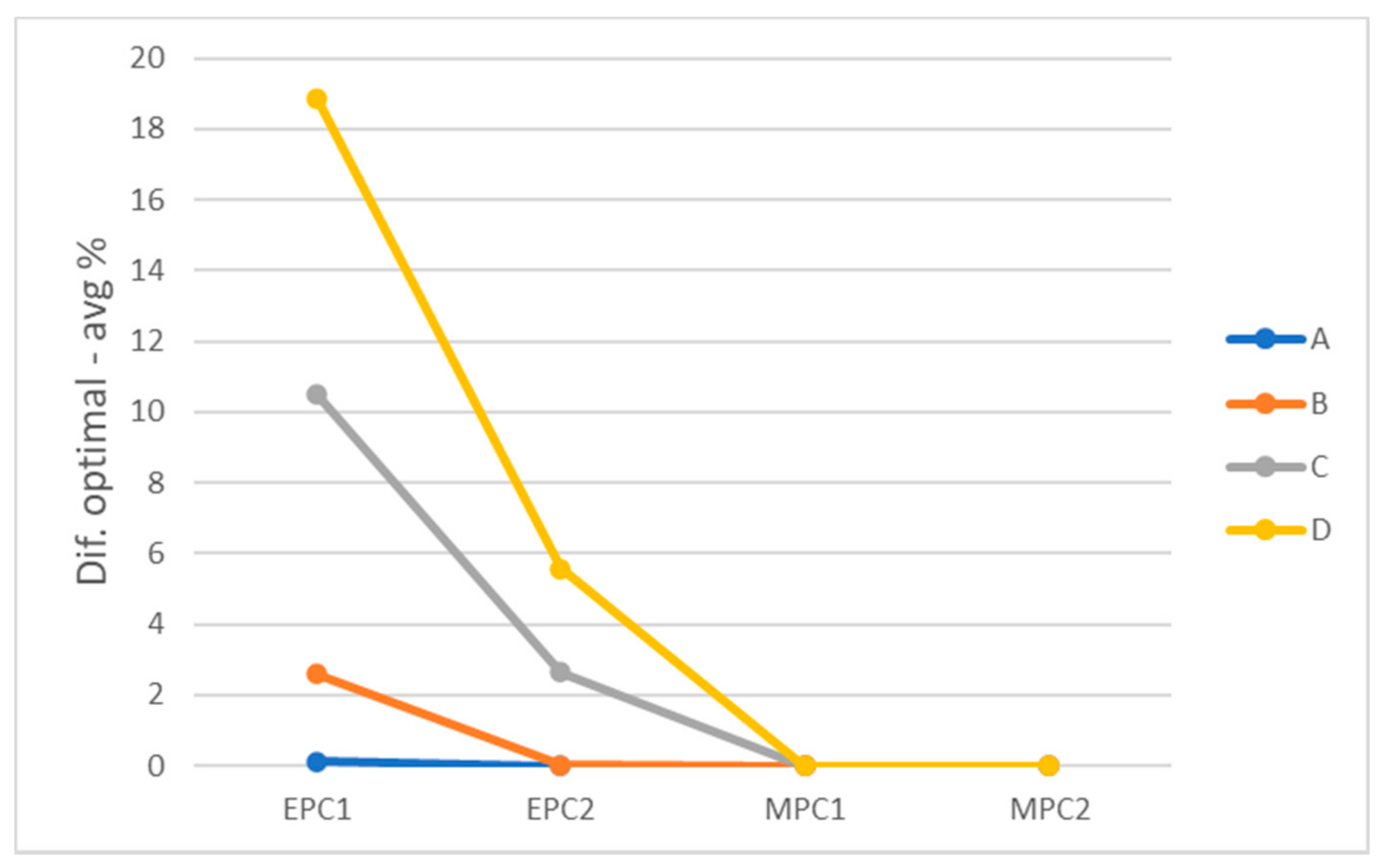
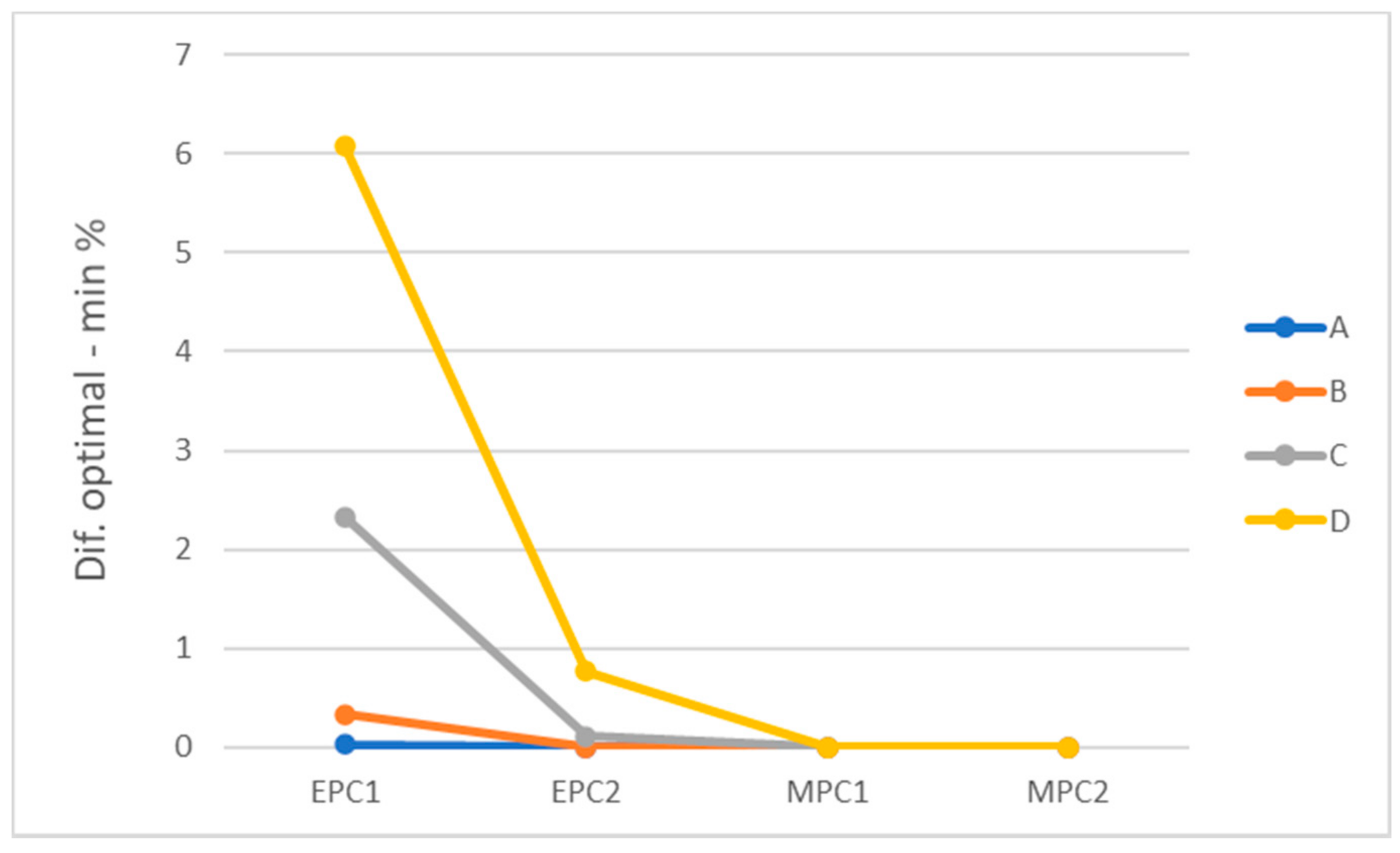
The values Standard deviation, Dif. optimal-avg and Dif. optimal-min can be used for illustration of the influence of HW used and method too. For all values, a smaller value is better. Figure 8 presents decreasing value of Standard deviation, Figure 9 presents decreasing value of Dif. optimal-avg and Figure 10 decreasing value of Dif. optimal-min. The best visibility of influence is mainly for benchmark D.
The advantage of performing a larger number of calculations on more powerful HW when using Solver is also evident from the histograms of benchmark D on Figure 4. The metaheuristic method has the same result on both PCs; for the evolutionary method there is an obvious difference in the quality of the results obtained on PC1 and PC2.
5. Conclusions
The obtained results show that the use of the Excel-Solver software for solving MFLP tasks is possible. The accuracy of the results depends on the complexity of the task and the HW used. Improving the results can be achieved by repeating the calculations and finding the lowest value in the result set. Even for the most demanding task from the used benchmarks, a deviation of the best solution from the optimal one of less than 1 percent can be achieved. In a real environment, it will not be possible to place the device exactly in the calculated locations, so these results can be considered accurate enough. Very good results have been achieved on the example of practice.
The use of the proposed method is especially suitable in situations where finding a solution is required and access to sophisticated methods for solving MFLP-type tasks is not possible. In education, it offers to acquaint students with the simple possibility of solving this type of problem and thus enable a wider use of optimization procedures in their future practice.
Author Contributions
Conceptualization, P.N.; methodology, P.N. and P.S.; software, P.N. and P.S.; validation, P.N.; formal analysis, P.N.; investigation, P.N.; resources, P.N.; data curation, P.N. and P.S.; Writing—Original draft preparation, P.N. and P.S.; visualization, P.N.; supervision, P.S.; project administration, P.N.; funding acquisition, P.N. All authors have read and agreed to the published version of the manuscript.
Funding
This research received no external funding.
Institutional Review Board Statement
Not applicable.
Informed Consent Statement
Not applicable.
Conflicts of Interest
The authors declare no conflict of interest.
References
- Erdoğan, G.; Stylianou, N.; Vasilakis, C. An open source decision support system for facility location analysis. Decis. Support Syst. 2019, 125, 113116. [Google Scholar] [CrossRef]
- Baj-Rogowska, A. “Selecting the Optimum Location for Logistics Facilities Using Solver—Case Study”. SSRN Scholarly Paper, ID 2883827, Social Science Research Network. 3 June 2016. Available online: https://papers.ssrn.com/abstract=2883827 (accessed on 24 March 2021).
- Wang, B.; Fu, X.; Chen, T.; Zhou, G. Modeling Supply Chain Facility Location Problem and Its Solution Using a Genetic Algorithm. J. Softw. 2014, 9, 2335–2341. [Google Scholar] [CrossRef]
- Wesolowsky, G.O.; Love, R.F. A Nonlinear Approximation Method for Solving a Generalized Rectangular Distance Weber Problem. Manag. Sci. 1972, 18, 656–663. [Google Scholar] [CrossRef]
- Dax, A. An Efficient Algorithm for Solving the Rectilinear Multifacility Location Problem. IMA J. Numer. Anal. 1986, 6, 343–355. [Google Scholar] [CrossRef]
- Idrissi, H.; Lefebvre, O.; Michelot, C. Duality for constrained multifacility location problems with mixed norms and applications. Ann. Oper. Res. 1989, 18, 71–92. [Google Scholar] [CrossRef]
- Francis, R.L.; McGinnis, F., Jr.; White, J.A. Facility Layout and Location: An Analytical Approach, 2nd ed.; Prentice Hall: Upper New Jersey River, NJ, USA, 1992. [Google Scholar]
- Calamai, P.; Charalambous, C. Solving multifacility location problems involving euclidean distances. Nav. Res. Logist. Q. 1980, 27, 609–620. [Google Scholar] [CrossRef]
- Chatelon, J.; Hearn, D.; Lowe, T.J. A Subgradient Algorithm for Certain Minimax and Minisum Problems—The Constrained Case. SIAM J. Control Optim. 1982, 20, 455–469. [Google Scholar] [CrossRef]
- Xue, G.-L. A globally convergent algorithm for facility location on a sphere. Comput. Math. Appl. 1994, 27, 37–50. [Google Scholar] [CrossRef] [Green Version]
- Juel, H.; Love, R.F. Sufficient Conditions for Optimal Facility Locations to Coincide. Transp. Sci. 1980, 14, 125–129. [Google Scholar] [CrossRef]
- Xue, G.; Rosen, J.; Pardalos, P. A polynomial time dual algorithm for the Euclidean multifacility location problem. Oper. Res. Lett. 1996, 18, 201–204. [Google Scholar] [CrossRef]
- Morris, J.G. A Linear Programming Approach to the Solution of Constrained Multi-Facility Minimax Location Problems where Distances are Rectangular. J. Oper. Res. Soc. 1973, 24, 419–435. [Google Scholar] [CrossRef]
- Drezner, Z.; Wesolowsky, G.O. A Trajectory Method for the Optimization of the Multi-Facility Location Problem WithlpDistances. Manag. Sci. 1978, 24, 1507–1514. [Google Scholar] [CrossRef]
- Sherali, H.D.; Shetty, C.M. A Primal Simplex Based Solution Procedure for the Rectilinear Distance Multifacility Location Problem. J. Oper. Res. Soc. 1978, 29, 373–381. [Google Scholar] [CrossRef]
- Dhar, U.R.; Rao, J.R. Domain Approximation Method for Solving Multifacility Location Problems on a Sphere. J. Oper. Res. Soc. 1982, 33, 639–645. [Google Scholar] [CrossRef]
- Aykin, T.; Babu, A.J.G. Multifacility location problems on a sphere. Int. J. Math. Math. Sci. 1987, 10, 583–595. [Google Scholar] [CrossRef]
- Vergin, R.C.; Rogers, J.D. An Algorithm and Computational Procedure for Locating Economic Facilities. Manag. Sci. 1967, 13, 240. [Google Scholar] [CrossRef]
- Pour, H.D.; Nosraty, M. Solving the facility and layout and location problem by ant-colony optimization-meta heuristic. Int. J. Prod. Res. 2006, 44, 5187–5196. [Google Scholar] [CrossRef]
- Lai, C.-M.; Chiu, C.-C.; Liu, W.-C.; Yeh, W.-C. A novel nondominated sorting simplified swarm optimization for multi-stage capacitated facility location problems with multiple quantitative and qualitative objectives. Appl. Soft Comput. 2019, 84, 105684. [Google Scholar] [CrossRef]
- Karimi, B.; Niknamfar, A.H.; Gavyar, B.H.; Barzegar, M.; Mohtashami, A. Multi-objective multi-facility green manufacturing closed-loop supply chain under uncertain environment. Assem. Autom. 2019, 39, 58–76. [Google Scholar] [CrossRef]
- Gao, X.; Zhou, Y.; Amir, M.I.H.; Rosyidah, F.A.; Lee, G.M. A Hybrid Genetic Algorithm for Multi-emergency Medical Service Center Location-allocation Problem in Disaster Response. Int. J. Ind. Eng. 2017, 24, 663–679. [Google Scholar]
- Liu, Z.; Li, H.; Gao, P. Multi-facilities Location and Allocation Problem of Three-Echelon Supply Chain Based on an Improved Genetic Algorithm. In Proceedings of the 2016 IEEE 13th International Conference on e-Business Engineering (ICEBE), Macau, China, 4–6 November 2016; Institute of Electrical and Electronics Engineers (IEEE): Piscataway, NJ, USA, 2016; pp. 139–144. [Google Scholar]
- Ismail, M.A.; Gomaa, A.H.; Nassef, A.O. Solving the Multi-Objective Facility Layout Problem Using Evolutionary Multi-Objective Optimization Algorithms. Manuf. Sci. Eng. 2006, 547–555. [Google Scholar] [CrossRef]
- Foltin, P.; Vlkovský, M.; Mazal, J.; Husák, J.; Brunclík, M. Discrete Event Simulation in Future Military Logistics Applications and Aspects. In Privacy Enhancing Technologies; Metzler, J.B., Ed.; Springer: Berlin/Heidelberg, Germany, 2018; Volume 10756, pp. 410–421. [Google Scholar]
- Stodola, P.; Mazal, J. Tactical Decision Support System to Aid Commanders in their Decision-Making. In Proceedings of the Modelling and Simulation for Autonomous Systems, Rome, Italy, 15–16 June 2016; pp. 396–406. [Google Scholar]
- Stodola, P.; Drozd, J.; Šilinger, K.; Hodický, J.; Procházka, D. Collective Perception Using UAVs: Autonomous Aerial Reconnaissance in a Complex Urban Environment. Sensors 2020, 20, 2926. [Google Scholar] [CrossRef]
- Blaha, M.; Šilinger, K. Application support for topographical-geodetic issues for tactical and technical control of artillery fire. Int. J. Circuits Syst. Signal Process. 2018, 12, 48–57. [Google Scholar]
- Hošková-Mayerová, Š.; Talhofer, V.; Otřísal, P.; Rybanský, M. Influence of Weights of Geographical Factors on the Results of Multicriteria Analysis in Solving Spatial Analyses. ISPRS Int. J. Geo-Inf. 2020, 9, 489. [Google Scholar] [CrossRef]
- Mazal, J.; Rybanský, M.; Bruzzone, A.G.; Kutěj, L.; Scurek, R.; Foltin, P.; Zlatník, D. Modelling of the microrelief impact to the cross country movement. Int. Conf. Harb. Marit. Multimodal Logist. Modeling Simul. 2020, 66–70. [Google Scholar] [CrossRef]
- Františ, P.; Hodický, J. Virtual reality in presentation layer of C3I system. In Proceedings of the MODSIM05—International Congress on Modelling and Simulation: Advances and Applications for Management and Decision Making, Proceedings 2005, Melbourne, Australia, 12–15 December 2005; pp. 3045–3050. [Google Scholar]
- Frantis, P.; Hodicky, J. Human machine interface in command and control system. In Proceedings of the 2010 IEEE International Conference on Virtual Environments, Human-Computer Interfaces and Measurement Systems, Taranto, Italy, 6–8 September 2010; Institute of Electrical and Electronics Engineers (IEEE): Piscataway, NJ, USA, 2010; Volume 1, pp. 38–41. [Google Scholar]
Figure 1.
Examples of benchmark instances: (a) instance A; (b) instance D.

Figure 2.
Visualization of benchmark instance E.

Figure 3.
Graphical comparison of benchmark complexity.

Figure 4.
Histograms.

Figure 5.
Best solution found by different methods using different hardware configurations.

Figure 6.
Representation of the best solution on map, left-only centers, right-centers and connected points.
Figure 6.
Representation of the best solution on map, left-only centers, right-centers and connected points.

Figure 7.
Influence of the complexity of the benchmark.

Figure 8.
Standard deviation for different configurations.

Figure 9.
Dif. optimal-avg for different configurations.

Figure 10.
Dif. optimal-min for different configurations.


Table 1.
Coordinates of points for instance E.
| 1,007,667 | 801,321 | 1,034,425 | 791,499 | 1,154,708 | 568,789 |
| 1,119,519 | 735,319 | 1,121,206 | 545,377 | 1,071,254 | 676,371 |
| 1,071,043 | 646,830 | 974,653 | 687,137 | 1,155,563 | 630,925 |
| 1,151,798 | 714,704 | 1,087,661 | 497,018 | 1,128,561 | 792,632 |
| 1,128,044 | 512,236 | 1,131,202 | 523,717 | 1,033,047 | 722,781 |
| 1,123,192 | 537,368 | 1,134,304 | 557,970 | 1,160,625 | 598,196 |
| 1,168,146 | 570,806 | 1,061,233 | 646,733 | 1,042,352 | 640,852 |
| 1,071,757 | 778,926 | 1,106,717 | 834,552 | 1,036,069 | 616,768 |
| 1,130,697 | 751,389 | 1,047,521 | 742,126 | 1,098,638 | 587,366 |
Table 2.
Benchmark instances.
| Benchmark Instance | Number of Points | Number of Centers | Optimal Solution |
|---|---|---|---|
| A | 25 | 5 | 28.284271 |
| B | 50 | 10 | 56.568542 |
| C | 75 | 15 | 84.852814 |
| D | 100 | 20 | 113.137085 |
| E | 27 | 4 | NA |
Table 3.
Parameters used for optimization in the Excel Solver.
| Parameter | Value |
|---|---|
| Max time | Unlimited |
| Iterations | Unlimited |
| Constraint precisions | 0.000001 |
| Convergence | 0.0001 |
| Population size | 100 |
| Random seed | 0 |
| Mutation rate | 0.075 |
| Maximum time without improvement | 30 s |
| Max subproblems | Unlimited |
| Maximum feasible solutions | Unlimited |
| Integer optimality | 1% |
Table 4.
Definitions of terms used.
| Name of Term | Explanation |
|---|---|
| Optimal | Optimal solution for an instance. As the optimal solution for instance E is not known, the minimal distance computed by metaheuristic algorithm is used. |
| Minimal | Minimal value from set of 100 results |
| Average | Average value from set of 100 results |
| Dif. optimal-min | Difference between optimal and minimal value (%) |
| Dif. optimal-avg | Difference between optimal and average value (%) |
| Standard dev. | Standard deviation for set of 100 results |
| Avg. time | Average time of computing one result in set of 100 results |
Table 5.
Definitions of abbreviations used.
| Name of Acronym | Explanation |
|---|---|
| EPC1 | Results of operations with evolutionary method on PC1 |
| EPC2 | Results of operations with evolutionary method on PC2 |
| MPC1 | Results of operations with metaheuristic algorithm on PC1 |
| MPC2 | Results of operations with metaheuristic algorithm on PC2 |
Table 6.
Calculations EPC1.
| Benchmark Instance | A | B | C | D | E |
|---|---|---|---|---|---|
| Optimal | 28.28427125 | 56.56854249 | 84.85281374 | 113.137085 | 990,045.8509 |
| Minimal | 28.29374372 | 56.76059189 | 86.82870516 | 120.0158802 | 990,062.7347 |
| Average | 28.31897317 | 58.04046807 | 93.7668965 | 134.4582737 | 993,877.2199 |
| Dif. optimal-min (%) | 0.0334903 | 0.3394986 | 2.3286104 | 6.0800534 | 0.0017054 |
| Dif. optimal-avg (%) | 0.1226898 | 2.6020214 | 10.5053473 | 18.8454464 | 0.3869891 |
| Standard dev. | 0.018928149 | 2.540417719 | 4.543094057 | 6.225660536 | 11868.19002 |
| Avg. time | 0:00:52 | 0:01:13 | 0:01:13 | 0:01:18 | 0:00:16 |
Table 7.
Calculations MPC1.
| Benchmark Instance | A | B | C | D | E |
|---|---|---|---|---|---|
| Optimal | 28.28427125 | 56.56854249 | 84.85281374 | 113.137085 | 990,045.8509 |
| Minimal | 28.284385 | 56.568868 | 84.853428 | 113.138157 | 990,045.8509 |
| Average | 28.28451488 | 56.56943484 | 84.85454469 | 113.1398439 | 990,046.998 |
| Dif. optimal-min (%) | 0.0004022 | 0.0005754 | 0.0007239 | 0.0009475 | 100 |
| Dif. optimal-avg (%) | 0.0008614 | 0.0015775 | 0.0020399 | 0.0024385 | 0.0001159 |
| Standard dev. | 7.87572 × 10⁻⁵ | 0.001088538 | 0.00246765 | 0.003354359 | 2.501989537 |
| Avg. time | 0:00:01.54384 | 0:00:06.45815 | 0:00:12.75186 | 0:00:20.99911 | 0:00:01.63003 |
Table 8.
Calculations EPC2.
| Benchmark Instance | A | B | C | D | E |
|---|---|---|---|---|---|
| Optimal | 28.28427125 | 56.56854249 | 84.85281374 | 113.137085 | 990,045.8509 |
| Minimal | 28.28427792 | 56.57242216 | 84.95282029 | 114.0087084 | 990,067.9344 |
| Average | 28.28446167 | 56.58777854 | 87.10410699 | 119.455867 | 993,753.3223 |
| Dif. optimal-min (%) | 0.0000236 | 0.0068583 | 0.1178589 | 0.7704135 | 0.0022306 |
| Dif. optimal-avg (%) | 0.0006732 | 0.0340048 | 2.6531745 | 5.585067 | 0.3744747 |
| Standard dev. | 0.000234536 | 0.009084584 | 3.490989067 | 4.547461935 | 11,876.6897 |
| Avg. time | 0:00:46 | 0:00:48 | 0:00:53 | 0:00:56 | 0:00:02 |
Table 9.
Calculations MPC2.
| Benchmark Instance | A | B | C | D | E |
|---|---|---|---|---|---|
| Optimal | 28.28427125 | 56.56854249 | 84.85281374 | 113.137085 | 990,045.8509 |
| Minimal | 28.284349 | 56.568848 | 84.853562 | 113.138194 | 990,045.8509 |
| Average | 28.28450837 | 56.56944912 | 84.85552771 | 113.1440408 | 990,046.9157 |
| Dif. optimal-min (%) | 0.0002749 | 0.0005401 | 0.0008818 | 0.0009802 | 100 |
| Dif. optimal-avg (%) | 0.0008384 | 0.0016027 | 0.0031984 | 0.0061481 | 0.0001076 |
| Standard dev. | 7.99256 × 10⁻⁵ | 0.001443795 | 0.006354751 | 0.027984218 | 2.973050376 |
| Avg. time | 0:00:00.4348 | 0:00:01.3472 | 0:00:02.91475 | 0:00:04.95436 | 0:00:00.81313 |
Table 10.
Best solution found for benchmark E.
| 1,057,779.759 | 647,144.3178 |
| 1,134,043.286 | 556,787.3659 |
| 1,130,696.403 | 751,390.0041 |
| 1,041,239.67 | 769,037.2559 |
Publisher’s Note: MDPI stays neutral with regard to jurisdictional claims in published maps and institutional affiliations. |
© 2021 by the authors. Licensee MDPI, Basel, Switzerland. This article is an open access article distributed under the terms and conditions of the Creative Commons Attribution (CC BY) license (http://creativecommons.org/licenses/by/4.0/).
Share and Cite
MDPI and ACS Style
Němec, P.; Stodola, P. Optimization of the Multi-Facility Location Problem Using Widely Available Office Software. Algorithms 2021, 14, 106. https://0-doi-org.brum.beds.ac.uk/10.3390/a14040106
AMA Style
Němec P, Stodola P. Optimization of the Multi-Facility Location Problem Using Widely Available Office Software. Algorithms. 2021; 14(4):106. https://0-doi-org.brum.beds.ac.uk/10.3390/a14040106
Chicago/Turabian StyleNěmec, Petr, and Petr Stodola. 2021. "Optimization of the Multi-Facility Location Problem Using Widely Available Office Software" Algorithms 14, no. 4: 106. https://0-doi-org.brum.beds.ac.uk/10.3390/a14040106
Note that from the first issue of 2016, this journal uses article numbers instead of page numbers. See further details here.