
Research on Optimization of Multi-Objective Regional Public Transportation Scheduling


School of Traffic & Transportation Engineering, Lanzhou Jiaotong University, Lanzhou 730070, China
*
Author to whom correspondence should be addressed.
Algorithms 2021, 14(4), 108; https://0-doi-org.brum.beds.ac.uk/10.3390/a14040108
Submission received: 25 February 2021
/
Revised: 23 March 2021
/
Accepted: 26 March 2021
/
Published: 28 March 2021
Abstract
:The optimization of bus scheduling is a key method to improve bus service. So, the purpose of this paper is to address the regional public transportation dispatching problem, while taking into account the association between the departure time of buses and the waiting time of passengers. A bi-objective optimization model for regional public transportation scheduling is established to minimize the total waiting cost of passengers and to maximize the comprehensive service rate of buses. Moreover, a NSGA-II algorithm with adaptive adjusted model for crossover and mutation probability is designed to obtain the Pareto solution set of this problem, and the entropy weight-TOPSIS method is utilized to make a decision. Then the algorithms are compared with examples, and the results show that the model is feasible, and the proposed algorithms are achievable in solving the regional public transportation scheduling problem.
1. Introduction
With the continuous expansion of urban space scale and population, public transportation has become a travel choice for more and more people. On ordinary weekdays, the number of public transport trips in Beijing is about 6.1 million people/day, accounting for 30% of the city’s permanent resident population, and on weekends, it is about 4.4 million people/day. Among them, the proportion of the direct bus travel is only 43.1% [1]. However, the lack of regional public transportation coordinated dispatching tends to result in a consequent worsening of both the magnitude and variability of the average waiting time. This in turn impacts heavily impacts the level of service. Owing to the inconvenience of transfer, public transportation in China is not attractive to travelers. Some studies have shown that transfer is one of the main factors that affect the travel rate of public transportation [2]. The travel time with transfer is obviously longer than the travel time without transfer in Beijing. The average time of a trip in the public transportation system is about 1 h, and the transfer time is more than 10 min [1,3]. So, it is necessary to study the coordinated dispatching problem of regional public transportation to reduce the transfer waiting time of passengers and improve the service level of public transportation.
2. Literature Review
Compared with single-line public transportation dispatching, regional public transportation dispatching can make public resources more fully utilized [4,5]. Transfer is the main factor of regional public transportation scheduling, and synchronous optimization of regional public transportation timetable can improve the transfer efficiency. Therefore, some researchers have studied the problem of synchronous transfer of regional public transportation scheduling. Liebchen and Stiller [6] considered the bus timetable affected by running late to achieve the optimization of departure interval and fleet size. Liu and Shen [7] established a bilevel programming model between the timetable generation and vehicle scheduling in the bus scheduling system according to the regional public transport scheduling mode. Ceder, Golany and Tal [8] established a collaborative optimization model to maximize the number of buses arriving at the station synchronously in the region. Ibarra-Rojas and Rios-Solis [9] optimized the departure schedule under the determination of the synchronous transfer time window to maximize the synchronous number. Eranki [10] considered the problem of developing synchronized timetables for bus transit systems with fixed routes to have maximum number of simultaneous arrivals. Wei, Chen, and Sun [11] optimized the departure schedule based on the shortest waiting time of passengers and the maximum number of bus berths. Liu et al. [12] evaluated the degree of synchronous bus arrival by defining the synergetic coefficient. Nesheli and Ceder [13] took the total travel time as the target and adopts the synchronous transfer problem of buses under different strategies. Hu, Zhao and Wang [14] realized synchronous transfer between urban bus lines and rural bus lines by optimizing the vehicle arrival time of transfer routes. Wagale et al. [15] presented a model to optimize the bus scheduling by taking into consideration of both bus stop and route segments of the city. Taking into account congestion on the public transport system and works by considering elastic demand, Ibeas et al. [16] proposed an optimization model for designing the intervals and sizes of buses circulating on public transport networks by minimizing the system’s operating and user costs. Wang et al. [17] built an optimal model to schedule the departure time of each bus service with the objective of minimizing the average waiting time. Boyer, Ibarra-Rojas and Ríos-Solís [18] dealt with the flexible vehicle and crew scheduling problem faced by urban bus transport agencies. Kumar, Prasath and Vanajakshi [19] proposed a demand and travel time responsive model to maximize the benefit of the operator by preparing an optimal schedule. Kang, Chen and Meng [20] developed three explicit integer linear programming models to formulate: the bus driver scheduling, bus and driver scheduling, and bus and driver scheduling with mealtime windows, respectively. Burdett et al. [21], Bevrani et al. [22,23], Ghaderi et al. [24] formulated some multi-objective capacity models to deal with transportation planning problem.
A review of the literature on regional public transport scheduling reveals that the existing research mainly considers the constraints on the waiting time for passengers, system’s operating cost or the degree of transfer synchronous. However, the losses of non-synchronized transfer passengers who choose to use alternative modes of transport because of the waiting and the bus capacity are rarely considered. The total waiting cost of passengers should include the waiting cost of passengers who have not achieved easy transfer and those who have to choose other modes of transportation, and the waiting time cost of non-transfer passengers. In terms of operating cost, departure frequency or full load rate are always considered. Effective operating time is also a major component of operating costs. In view of the above, this paper proposes a multi-objective optimization model of regional public transportation to minimize the total waiting cost of passengers and to maximize the comprehensive service rate of buses. According to the characteristics of this model, an improved NSGA-II algorithm is designed to obtain the Pareto solution set of this problem, and the entropy weight-TOPSIS method is used to make a decision.
The remainder of the paper is organized as follows: Some mathematical notations are defined in Section 3.1, and the bus operation process and passenger waiting time are analyzed in Section 3.2. A bi-objective optimization model for regional public transport scheduling is established in Section 3.3. The NSGA-II algorithm with adaptive adjusted model for crossover and mutation probability as the first step of the two-step algorithm is proposed in Section 4.1, and the entropy weight-TOPSIS method as the second step is implemented in Section 4.2. The proposed algorithm is tested via a numerical example in Section 5. Finally, the conclusions are given in Section 6.
3. The Regional Public Transportation Scheduling Model
Compared with traditional single-line public transportation dispatching, regional public transportation dispatching is more complicated. If only considering the number of easy transfer buses in the process of dispatching, it may lead to ignoring the transfer satisfaction of passengers at other transfer stations. So, the number of passengers who have not realized easy transfer at all the transfer stations should be taken into account so as to improve the service level of public transport.
Some assumptions involved in this paper are as follows:
- (1)
- The buses operating on each line are considered to be full-range buses.
- (2)
- There are no overtaking, stopovers and U-turns.
3.1. Notations
(1) Parameters
is the bus line, is the number of lines;
is the station set, represents station of line , and is the number of stations on line ;
is the set of pairs for transfer stations;
implies the bus x uses line i, where is the bus set;
is the passenger capacity of the bus;
denote the arrival number and alighting rate of passengers on the bus at station , respectively;
is the proportion of passenger transfer from line i to j at transfer-station ;
and indicate the number of passengers getting on and off the bus at station of line ;
is the number of passengers who failed to get on the bus of line at station ;
indicates the number of passengers on the bus of line at station ;
denotes the travel time from station to station , when , represents the time from the parking lot to the departure station;
indicates the dwelling time of bus of line at station ;
and indicate the time window for easy transfer;
indicates the time when the bus of line arrives at station ;
denotes the time when the bus of line leaves station ;
and are the scheduling simulation time window;
and indicate the minimum and maximum departure interval during the simulation;
indicates whether the bus of line j at station can be easily transferred to the bus of station on line i, where are the time window for synchronous transfer;
indicates the proportion of choice other transportation modes for passengers who are failed to get on the bus;
indicates the number of passengers who failed to get on the bus at the bus of line i at station and chose other transportation modes;
indicates whether the two lines can be transferred.
(2) Decision variables
indicates the departure time of bus of line from the parking lot.
3.2. Operation Analysis
(1) Analysis of bus operation process
The dwelling time of each bus can be expressed as , where is the time of buses to enter and leave the station, and indicate the average boarding and alighting time for each passenger, respectively.
The bus arrival time at the departure station can written as , where indicates the running time of line i from the parking lot to the departure station, and the bus departure time can be computed as .
The total running time of a bus can be calculated by .
(2) Passenger number analysis
The number of passengers getting off the bus is determined by the number of passengers on the bus, , and the alighting rate of passengers, , which can be calculated using
There are two aspects to consider in terms of the number of passengers getting on the bus: the remaining capacity of the bus and the number of passengers the who expect to board the bus which includes the number of people arriving randomly, the number of people who need to transfer, and the number of people who fail to get on the previous bus (do not include those who choose other modes of transportation). So, the number of passengers getting on the bus can be formulated as follows:
Then, the number of passengers on the bus at station, , is the number of passengers on the vehicle, , minus the number of passengers getting off the vehicle, , plus the number of passengers getting on the vehicle, which can be obtained:
In addition, the number of passengers who have not achieved easy transfer can be expressed as .
Thus, the number of passengers who fail to get on the bus is the number of passengers who need to get on the bus in the current period minus the number of passengers who actually get on the vehicle, which can be computed as follows:
(3) Analysis of passenger waiting time
The waiting time for transfer passengers is the arrival departure interval of two buses with transfer relationship multiplied by the number of transfer people with easy transfer, which can be calculated as follows:
Furthermore, the waiting time for non-transfer passengers includes the average waiting time of random arriving passengers and the extra waiting time of passengers who fail to get on the bus according to Larsen and Sunde [25], which can be calculated by
The ratio of the inter-station operating time of all buses to the total operating time is 1 minus the proportion of stop time, which can reflect the effective operation cost and can be expressed as:
3.3. The Optimization Model
Based on the above analysis, the first objective of this model is to minimize the total waiting cost of passengers who have not achieved easy transfer and those who have to choose other modes of transportation, and the waiting time cost of non-transfer passengers and transfer passengers. The second objective of this model is to consider the efficiency of public transport operation, including the average full load rate of buses and the ratio of inter-station running time of all buses to the total operation time. Then, the bi-objective optimization model for regional public transport scheduling can be formulated as follows:
s.t.
Formula (8) indicates the total waiting cost of passengers, represent the waiting cost coefficients of passengers who did not realize easy transfer and choose other modes of transportation, and the time value cost of waiting time. Formula (9) indicates the comprehensive service ratio of buses, is the number of elements of the set X. Constraint (10) ensures that the departure time is within the scheduling simulation time window. Constraint (11) is the bus capacity constraint. Constraint (12) indicates the arrival interval limits.
4. Solution Algorithms
As most of the multi-objective problems have to meet several objectives, it is impossible to obtain a unique solution that satisfies all the objectives simultaneously. Usually, Simulated Annealing (SA) [21], Ant Colony Optimization (ACO) [26], Multi-objective Heuristic Algorithms [27], Discrete Evolutionary Multi-objective Optimization (DEMO) [28], Niched Genetic Algorithm [5], Non-dominated Sorting Genetic Algorithm (NSGA) [29,30] are often chosen to solve multi-objective problems. One of the widely used algorithms proposed to solve multi-objective problems is the Non-dominated Sorting Genetic Algorithm-II (NSGA-II).
The scheduling of different bus lines will affect the transfer efficiency. Moreover, there are many schemes for each bus line and the two objectives conflict with each other. Therefore, it is necessary to design an algorithm that can deal with multi-objective public transportation scheduling quickly. In this section, a two-step algorithm is employed in order to solve this problem. The first step is to obtain the Pareto solutions, and the second step is to obtain a satisfactory scheme from the Pareto solution set on the basis of the entropy weight-TOPSIS method.
4.1. The NSGA-II Algorithm
The NSGA-II algorithm is one of the most commonly used multi-objective optimization algorithms, but it has some drawbacks of an uneven convergence of the population and the ease of falling into the local optimal solution [31]. In order to avoid premature convergence of Genetic algorithm, it is necessary to keep the diversity of population. According to the characteristics of this model, an adaptive adjusted model of the crossover and the mutation probability is introduced, and an adaptive crossover operator for judging the similarity of chromosomes and multipoint mutation operator are designed.
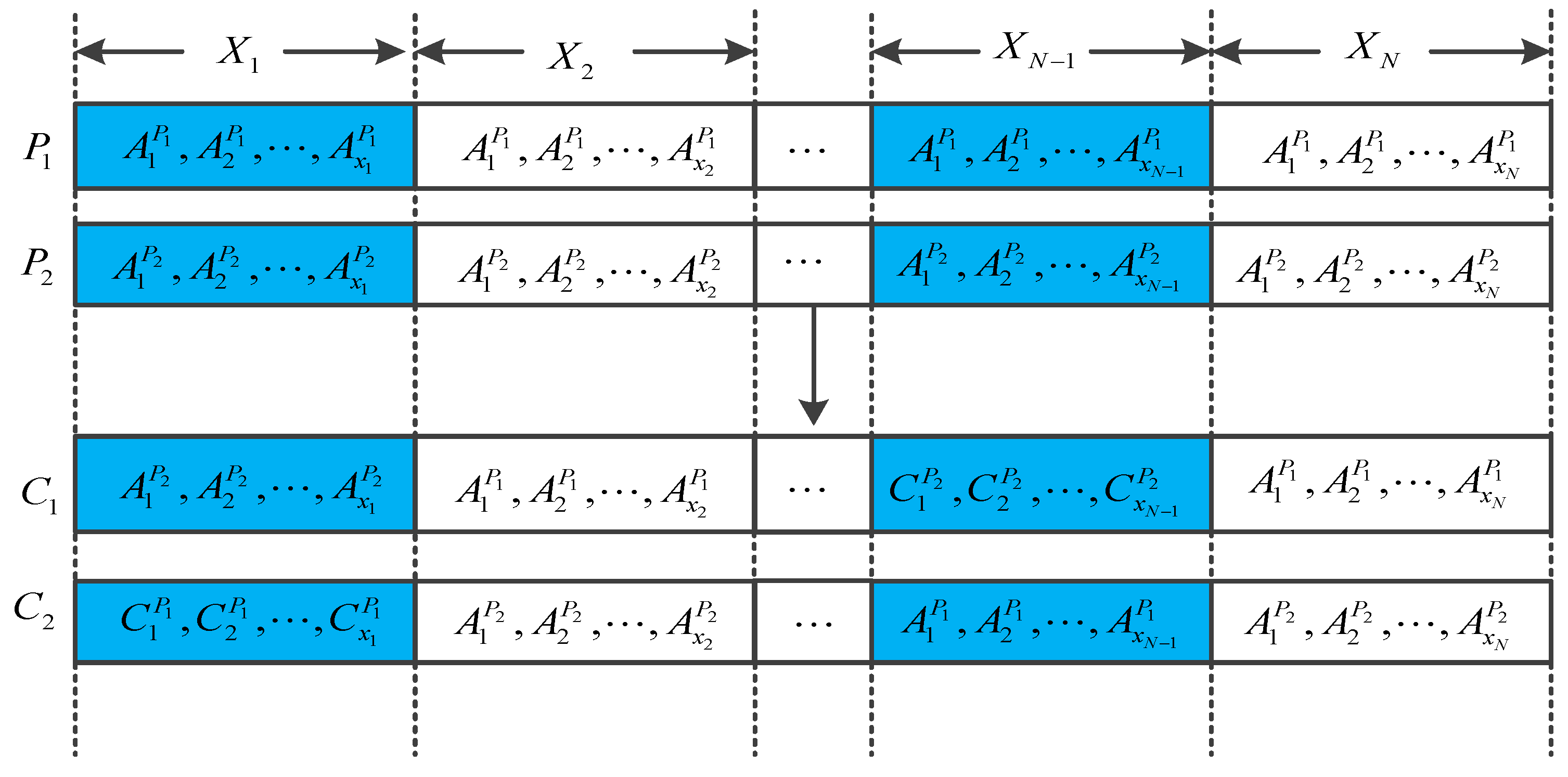
(1) Construction of chromosomes
Chromosome is designed by a positive integer, where gene of the chromosome represents the set of the departure time for each bus of line i. Figure 1 illustrates the specific structure of a randomized chromosome.
The process of generating a chromosome is as follows:
Step 1: Let and (where is a random number obeying 0–1 uniform distribution).
Step 2: , If , let , return to Step 2. Otherwise, go to Step 3.
Step 3: if , , return to Step 2. Otherwise, stop.
(2) Select operator
The selection of the parental population is using binary tournament method calculate the performing non-dominated sorting and crowding calculation of the parental population.
(3) Adaptive adjusted model for crossover and mutation probability
In order to improve the search performance of the algorithm and avoid falling into the local optimal solution, an adjusted model is adopted to adjust the crossover probability and mutation probability.
The crossover probability can be adjusted by the following method.
where , are the crossover probability for different generations, is the adjustment coefficient of crossover and mutation probability in the later stage of evolution. is the current evolutionary generation, are the dividing points of the early stage and the middle stage, and is the total maximum evolution generation.
Furthermore, the mutation probability can be adjusted by the following method according to the running phase.
where represents the total number of bus departures for all lines in a chromosome, is the maximum mutation probability.
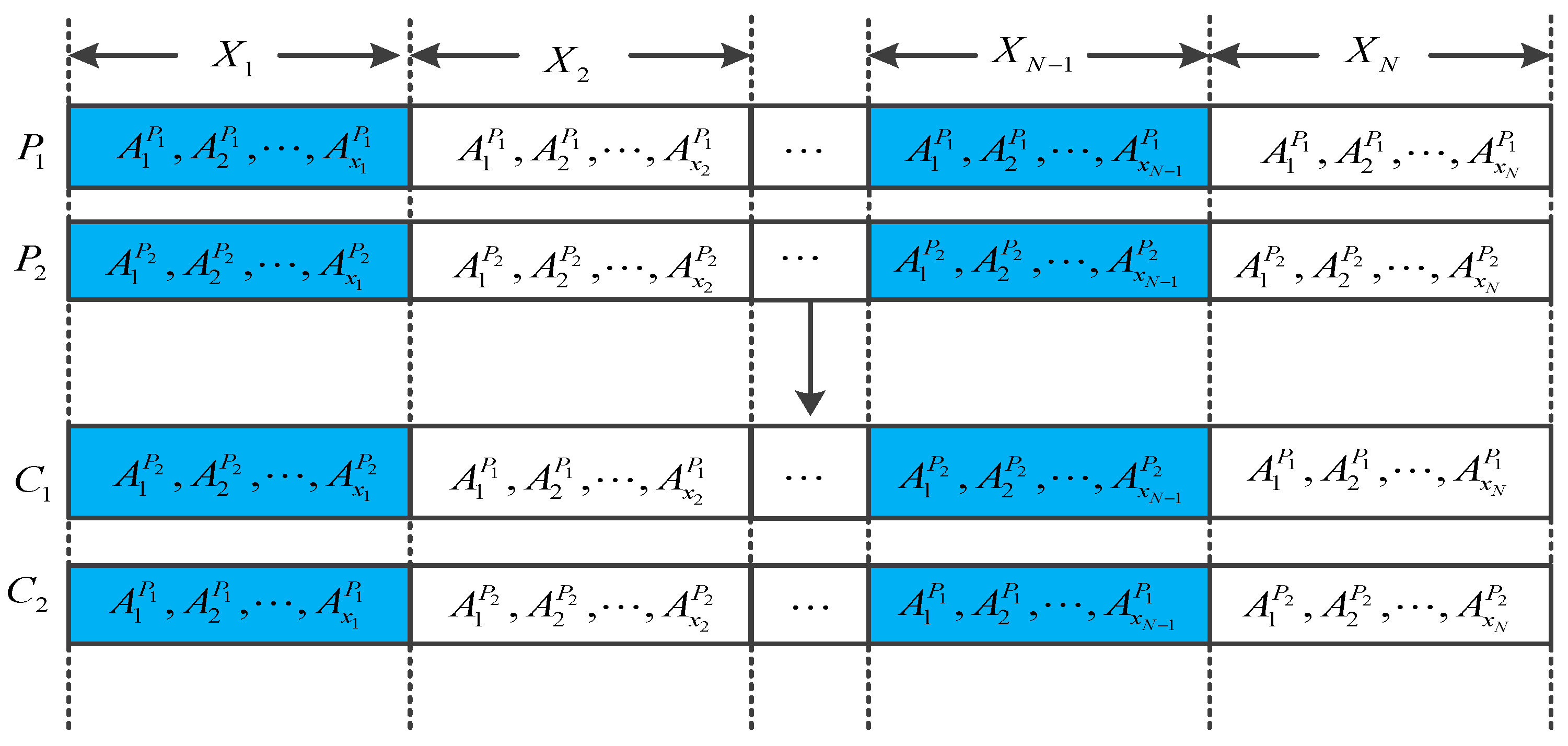
(4) Crossover operator
According to the character of the chromosome structure, the traditional single-point crossover is easy to fall into the local optimal solution. Therefore, an adaptive crossover operator is designed through judging the similarity of chromosomes.
The process of adaptive crossover operator is stated as follows:
Step1: Let .
Step2: If , then go to step 4. Otherwise, compare the number of bus departures of a line for the two selected chromosomes, if the departure times are equal, let the departure times of line be and go to Step3, otherwise, let , return to Step2.
Step3: Count the number of equal departure time of lines of the two chromosomes. If , then regenerate the departure time of line for one chromosome and exchange the genes of line of two chromosomes, and let , go to Step2.
Step4: If , randomly generate two different lines and exchange the corresponding genes of two chromosomes.
In the case of , the crossover process is shown in Figure 2. Assume that the first genes of parents are highly similar to the genes, then randomly select one chromosome from , regenerate the departure time of the high similarity line, and exchange the corresponding genes of (where is the regenerated departure time). The crossover process when is shown in Figure 3.
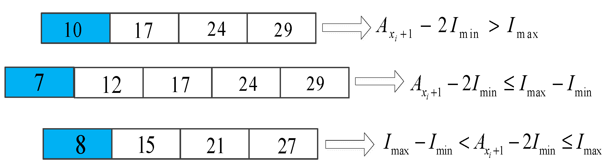
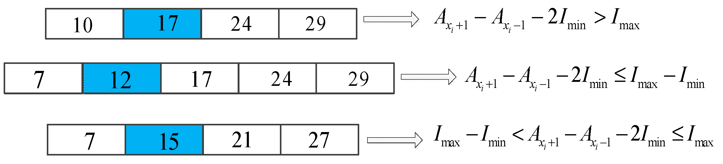
(5) Mutation operator
Randomly select two different lines from a chromosome and calculate the length of each line gene .
Randomly select some places form line gene and regenerate these departure time according to the following conditions (, and denote the departure time of bus and respectively, and indicates a random number from uniform distribution ).
Case 1: When , if , then . Otherwise, if , then , otherwise, .
Case 2: When , .
Case 3: When , if , then . Otherwise, if , then , otherwise .
4.2. Obtain Satisfactory Scheme from Pareto Solution Set
The second step is to obtain a satisfactory scheme from the Pareto solution set. The entropy weight-TOPSIS method is an improvement over the entropy weight method and the TOPSIS method [32]. Moreover, it is a common evaluation method used in multi-objective decision-making problems. Consequently, the entropy weight-TOPSIS method is used to obtain satisfactory schedule from the Pareto set.
Suppose that the number of Pareto solutions is M. Then, a decision matrix is obtained with M Pareto solutions and 2 objectives. The process is stated as follows:
Step 1: Obtaining the standardization matrix and normalized matrix .
Step 2: Calculating the information entropy of each objective j:
Step 3: Computing the weight of objective j:
Step 4: Computing the weighted judgment matrix:
Step 5: Calculating the Euclidean distance and closeness for each solution:
Moreover, the satisfactory schedule can be obtained according to the closeness .
5. Example Analysis
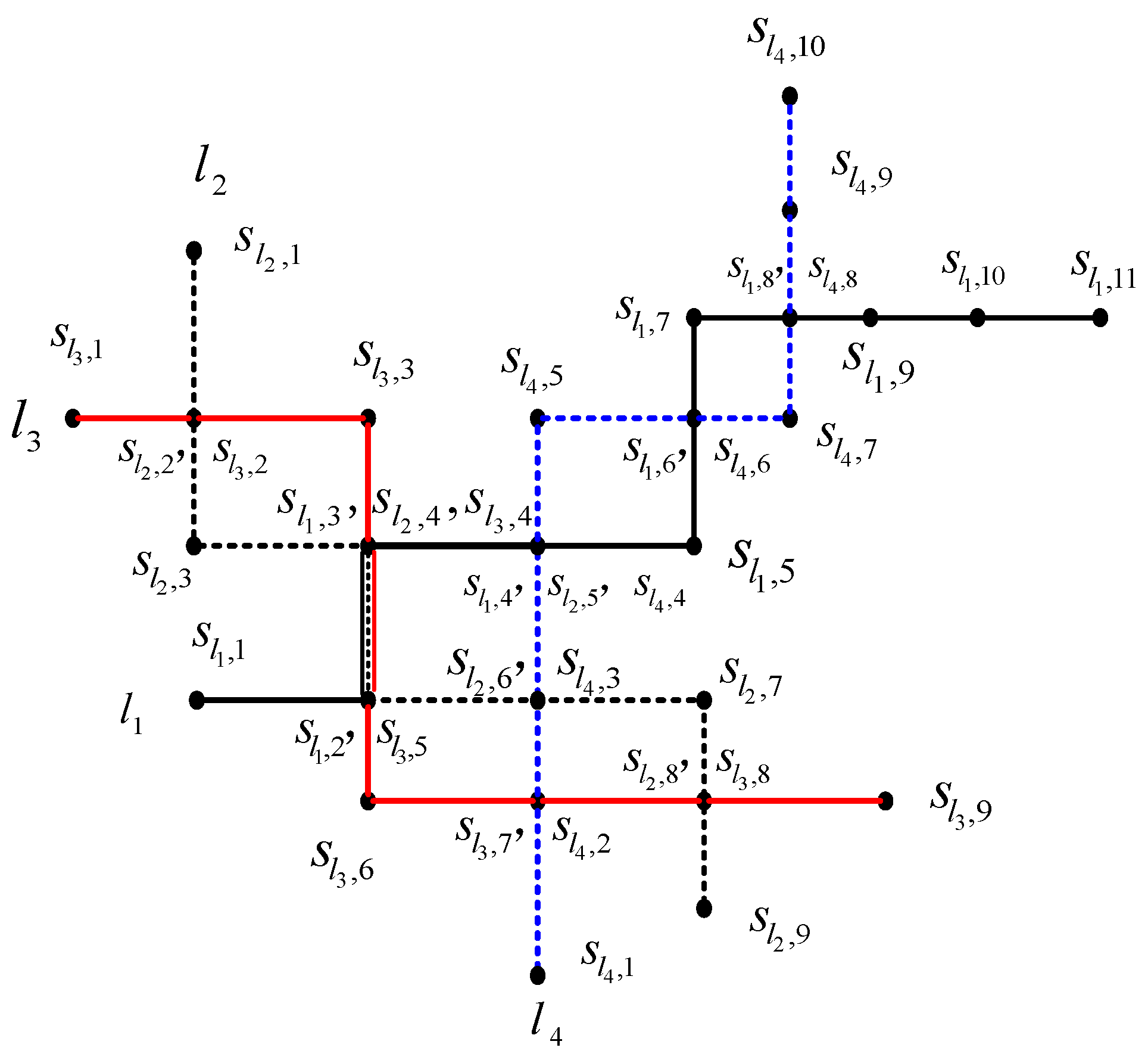
A case study is carried out to test the dispatch approach and algorithm on a regional public transportation network with four bus lines, as shown in Figure 6. The scheduling simulation time window and were set to be 7:00, 7:30, respectively. The minimum and maximum departure interval, and , were set to be 3 min, 10 min, and the time window for easy transfer, and , were 1 min and 5 min, respectively. Let the waiting cost coefficient , . The passenger capacity of the bus .
Based on the investigation of bus transfer stations in line 7, line 15 and line 131 of Lanzhou City, it is found that the more the number of passengers who failed to get on the bus, the higher the proportion of passengers who choose other modes of transportation. The corresponding proportion of choice other transportation modes for those passengers is as follows:
The size of population is 50, the maximum number of iterations is 150, the maximum mutation rate , and , . The main transfer stations and transfer proportions are shown in Table 1, and the average arrival rate, alighting rate of passengers and travel time between stations are listed in Table 2.
The Pareto solutions obtained and the weighted objective value of them are shown in Table 3, and the Euclidean distance between solutions and positive and negative ideal points and the closeness of solutions are listed in Table 4 after using the entropy-weight TOPSIS method. It can be seen from Table 4 that solution 7 is the most satisfactory operation schedule, and its operation schedule is given in Table 5.
By comparing solution 7 with the average value of schedules at a fixed departure interval of 3~10 min (as shown in Table 6), it can be seen that the total cost of loss for passengers is reduced by 31.42%, the comprehensive service ratio of buses is increased by 0.04%, and the number of passengers who not achieved easy transfer decreased by 74.29%.
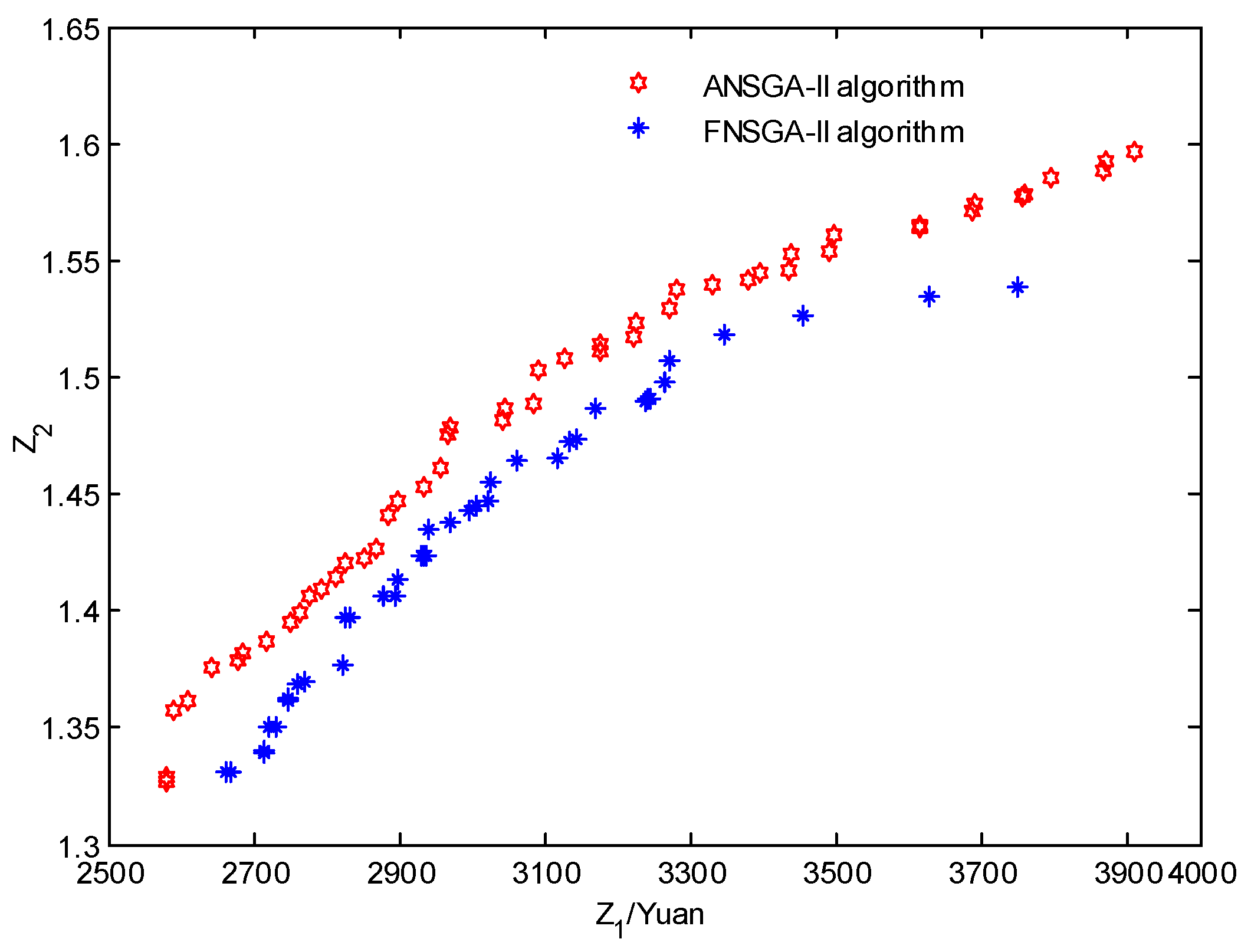
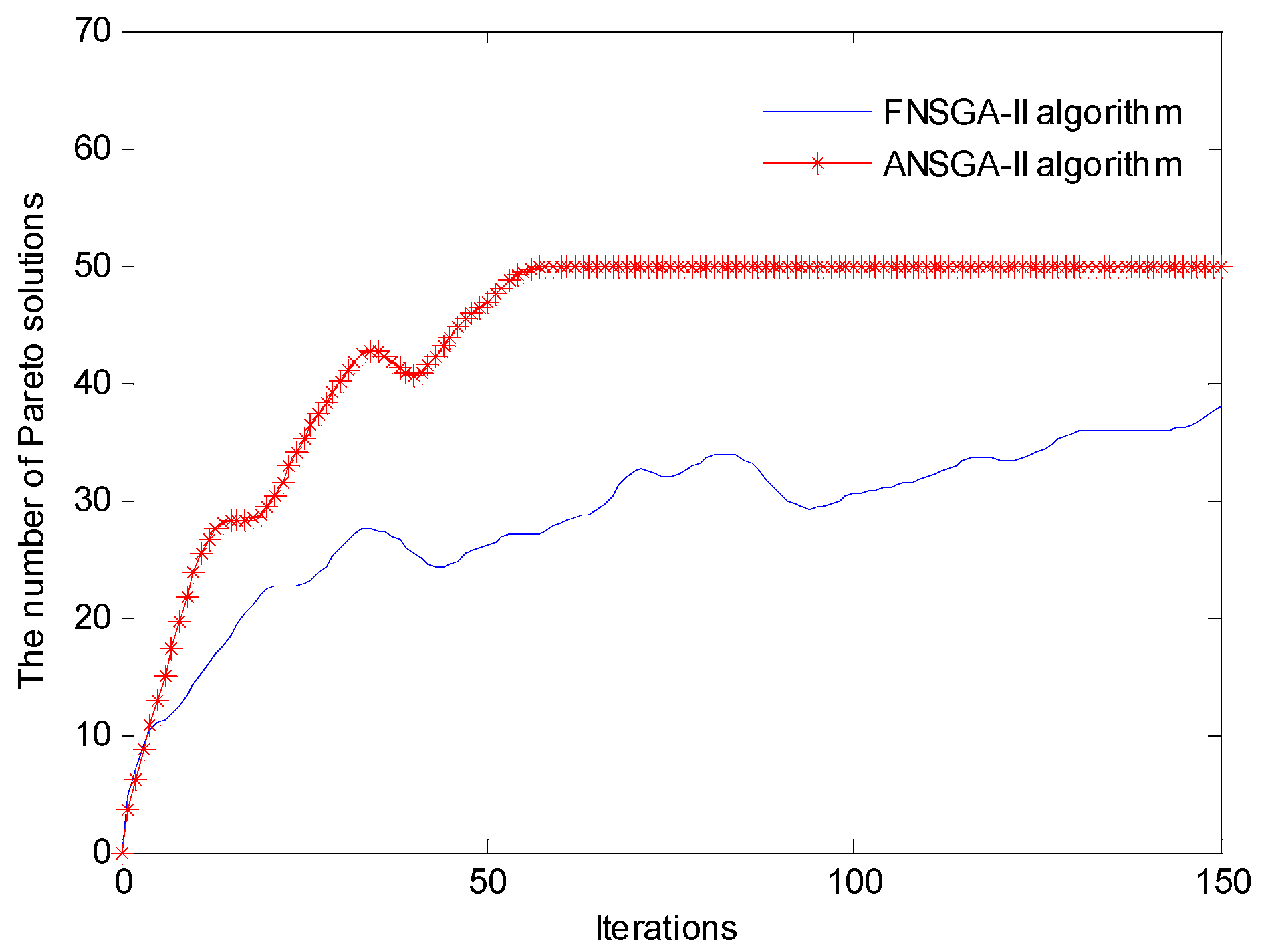
For comparing the performance of NSGA-II with the fixed crossover probability and mutation probability (FNSGA-II) and NSGA-II with adaptive adjusted model for crossover and mutation probability (ANSGA-II), the two algorithms solve the test experiment for 10 times. The Pareto solutions obtained of two algorithms after running 10 times are shown in Figure 7, and the number of nondominated set with different iterations of each algorithm is shown in Figure 8. The results show that the obtained solution set by ANSGA is superior to that obtained by FNSGA-II.
6. Conclusions
A bi-objective optimization model for regional public transport scheduling is established considering the total cost of passengers and the efficiency of public transport operation. Furthermore, a two-step algorithm is designed to solve this problem. In the first step, the NSGA-II algorithm with adaptive adjusted model for crossover and mutation probability is used to obtain the Pareto solutions. In the second step, the entropy weight-TOPSIS method is implemented to find a satisfactory scheme. At last, a regional public transportation network is collected to test the dispatch approach and algorithm. The results show that the scheduling scheme obtained in this paper is obviously better than the schemes with fixed departure interval, and the obtained solution set by ANSGA is superior to that obtained by FNSGA-II.
In this paper, we assumed that the running time between stations is known. In reality, the running time may be uncertain due to delay. Therefore, future research can consider the followings:
- (1)
- Considering the uncertainty of the running time to design the regional public transport scheduling model and algorithm.
- (2)
- Considering other factors, such as multiple types of buses, energy consumption, depots capacities, to the regional bus scheduling problem is studied, to research on the regional public transportation scheduling.
Author Contributions
Conceptualization, X.Y.; methodology, X.Y. and Y.Q.; software, X.Y.; validation, Y.Q.; formal analysis, X.Y.; investigation, Y.Q.; data curation, Y.Q.; writing—original draft preparation, Y.Q.; writing—review and editing, X.Y.; supervision, X.Y.; project administration, X.Y.; funding acquisition, X.Y. Both authors have read and agreed to the published version of the manuscript.
Funding
This research was funded by the National Natural Science Foundation of China, grant numbers 71761024.
Data Availability Statement
Data sharing is not applicable to this article.
Conflicts of Interest
The authors declare no conflict of interest.
References
- Beijing Transport Institute: Analysis on the Characteristics of Beijing Residents’ Public Transport Travel. Available online: https://mp.weixin.qq.com/s/oeK1d8iaqrRN8PS39smfyw (accessed on 5 June 2019).
- Fu, J.G. The Key Technologies research to improve transit trip rate. Urban Dev. Stud. 2014, 21, 79–83. [Google Scholar]
- Guo, Z.; Wilson, N.H.M. Assessing the cost of transfer inconvenience in public transport systems: A case study of the London underground. Transp. Res. Part A Policy Pract. 2011, 45, 91–104. [Google Scholar] [CrossRef]
- Wei, M.; Chen, X.W.; Sun, B. Multi-objective single line transit mixed scheduling model considering express bus Service. J. Transp. Syst. Eng. Inf. Technol. 2015, 15, 169–174. [Google Scholar]
- Yang, X.F.; Liu, L.F. A Multi-objective bus rapid transit energy saving dispatching optimization considering multiple types of vehicles. IEEE Access 2020, 8, 79459–79471. [Google Scholar] [CrossRef]
- Liebchen, C.; Stiller, S. Delay resistant timetabling. Public Transp. 2009, 1, 55–72. [Google Scholar] [CrossRef]
- Liu, Z.G.; Shen, J.S. Regional bus operation bi-level programming model integrating timetabling and vehicle scheduling. Syst. Eng. Theory Pract. 2007, 11, 135–141. [Google Scholar] [CrossRef]
- Ceder, A.; Golany, B.; Tal, O. Creating bus timetables with maximal synchronization. Transp. Res. Part A Policy Pract. 2001, 35, 913–928. [Google Scholar] [CrossRef]
- Ibarra-Rojas, O.J.; Rios-Solis, Y.A. Synchronization of bus timetabling. Transp. Res. Part B Methods 2012, 46, 599–614. [Google Scholar] [CrossRef]
- Eranki, A. A Model to Create Bus Timetables to Attain Maximum Synchronization Considering Waiting Times at Transfer Stops. Master’s Thesis, University of South Florida, Tampa, FL, USA, 2004. [Google Scholar]
- Wei, M.; Chen, X.W.; Sun, B. A model and an algorithm of schedule coordination for multi-mode regional bus transit. J. Highw. Transp. Res. Dev. 2015, 32, 136–142. [Google Scholar]
- Liu, Z.G.; Shen, J.S.; Wang, H.X.; Yang, W. Regional public transportation timetabling model with synchronization. J. Transp. Syst. Eng. Inf. Technol. 2007, 7, 109–113. [Google Scholar]
- Nesheli, M.M.; Ceder, A. Optimal combinations of selected tactics for public-transport transfer synchronization. Transp. Res. Part C Emerg. Technol. 2014, 48, 491–504. [Google Scholar] [CrossRef]
- Hu, B.Y.; Zhao, H.; Wang, D.X. Synchronous transfer model of urban public transport and rural passenger transport. J. Highw. Transp. Res. Dev. 2019, 13, 144–150. [Google Scholar]
- Wagale, M.; Singh, A.P.; Sarkar, A.K.; Arkatkar, S. Real-time optimal bus scheduling for a city using a DTR model. Procedia Soc. Behav. Sci. 2013, 104, 845–854. [Google Scholar] [CrossRef] [Green Version]
- Ibeas, A.; Alonso, B.; Dell’Olio, L.; Moura, J.L. Bus size and headways optimization model considering elastic demand. J. Transp. Eng. 2014, 140, 370–380. [Google Scholar] [CrossRef]
- Wang, Y.; Zhang, D.X.; Hu, L.; Yang, Y.; Lee, L.H. A data-driven and optimal bus scheduling model with time-dependent traffic and demand. IEEE Trans. Intell. Transp. Syst. 2017, 18, 2443–2452. [Google Scholar] [CrossRef]
- Boyer, V.; Ibarra-Rojas, O.J.; Ríos-Solís, Y.Á. Vehicle and crew scheduling for flexible bus transportation systems. Transp. Res. Part B Meth. 2018, 112, 216–229. [Google Scholar] [CrossRef]
- Kumar, B.A.; Prasath, G.H.; Vanajakshi, L. Dynamic bus scheduling based on real-time demand and travel time. Int. J. Civ. Eng. 2019, 17, 1481–1489. [Google Scholar] [CrossRef]
- Kang, L.J.; Chen, S.K.; Meng, Q. Bus and driver scheduling with mealtime windows for a single public bus route. Transp. Res. 2019, 101, 145–160. [Google Scholar] [CrossRef]
- Burdett, R.L. Multi-objective models and techniques for analysing the absolute capacity of railway networks. Eur. J. Oper. Res. 2015, 245, 489–505. [Google Scholar] [CrossRef] [Green Version]
- Bevrani, B.; Burdett, R.; Bhaskar, A.; Yarlagadda, P.K.D.V. A multi-criteria multi-commodity flow model for analysing transportation networks. Oper. Res. Perspect. 2020, 7, 100159. [Google Scholar] [CrossRef]
- Bevrani, B.; Burdett, R.L.; Yarlagadda, P.K.D.V. A capacity assessment approach for multi-modal transportation systems. Eur. J. Oper. Res. 2017, 263, 864–878. [Google Scholar] [CrossRef] [Green Version]
- Ghaderi, A.; Burdett, R.L. An integrated location and routing approach for transporting hazardous materials in a bi-modal transportation network. Transp. Res. Part E Logist. Transp. Rev. 2019, 127, 49–65. [Google Scholar] [CrossRef]
- Larsen, O.I.; Sunde, Ø. Waiting time and the role and value of information in scheduled transport. Res. Transp. Econ. 2008, 23, 41–52. [Google Scholar] [CrossRef]
- Xiang, W. A multi-objective ACO for operating room scheduling optimization. Nat. Comput. 2017, 16, 607–617. [Google Scholar] [CrossRef]
- Dulebenets, M.A.; Pasha, J.; Kavoosi, M.; Abioye, O.F.; Ozguven, E.E.; Moses, R.; Boot, W.R.; Sando, T. Multiobjective optimization model for emergency evacuation planning in geographical locations with vulnerable population groups. J. Manag. Eng. 2020, 36, 04019043. [Google Scholar] [CrossRef]
- Han, Y.Y.; Li, J.Q.; Sang, H.Y.; Liu, Y.P.; Gao, K.Z.; Pan, Q.K. Discrete evolutionary multi-objective optimization for energy-efficient blocking flow shop scheduling with setup time. Appl. Soft. Comput. 2020, 93, 106343. [Google Scholar] [CrossRef]
- Li, Y.Y.; Wang, S.Q.; Duan, X.B.; Liu, S.J.; Liu, J.P.; Hu, S. Multi-objective energy management for Atkinson cycle engine and series hybrid electric vehicle based on evolutionary NSGA-II algorithm using digital twins. Energy Convers. Manag. 2021, 230, 113788. [Google Scholar] [CrossRef]
- Liu, J.; Ma, B.; Zhao, H.B. Combustion parameters optimization of a diesel/natural gas dual fuel engine using genetic algorithm. Fuel 2020, 260, 116365. [Google Scholar] [CrossRef]
- Deb, K.; Pratap, A.; Agarwal, S. A fast and elitist multi-objective genetic algorithm: NSGA-II. IEEE Trans. Evol. Comput. 2002, 6, 182–197. [Google Scholar] [CrossRef] [Green Version]
- Luo, J.; Chen, S.Y.; Sun, X.; Zhu, Y.Y.; Zeng, J.X.; Chen, G.P. Analysis of city centrality based on entropy weight TOPSIS and population mobility: A case study of cities in the Yangtze River Economic Belt. J. Geogr. Sci. 2020, 30, 515–534. [Google Scholar] [CrossRef]
Figure 1.
An example of a chromosome.

Figure 2.
The crossover process case .

Figure 3.
The crossover process case .

Figure 4.
Illustration of the mutation operator for case 1.

Figure 5.
Illustration of the mutation operator for case 3.

Figure 6.
A regional public transportation network.

Figure 7.
Comparison of calculation results for two algorithms.

Figure 8.
The variation trend of non-dominated individuals.


Table 1.
Transfer station and transfer proportion.
| Transfer Station Pair | Transfer Proportion | Transfer Station | Transfer Proportion |
|---|---|---|---|
| 0.35 | 0.5 | ||
| 0.45 | 0.25 | ||
| 0.35 | 0.15 | ||
| 0.05 | 0.2 | ||
| 0.4 | 0.3 | ||
| 0.45 | 0.05 | ||
| 0.35 |
Table 2.
The average arrival rate, alighting rate of passengers and travel time between stations.
| 2 | 1 | 0 | 3 | 2 | 0.05 | 3.5 | 1 | 0.35 | ||||||
| 3.5 | 1 | 0.05 | 3 | 2 | 0.25 | 2 | 2 | 0.4 | ||||||
| 2.5 | 2 | 0.05 | 2.5 | 2 | 0.2 | 2.5 | 0 | 1 | ||||||
| 3.5 | 3 | 0.1 | 3 | 2 | 0.25 | 1.5 | 1 | 0 | ||||||
| 3 | 2 | 0.25 | 3 | 1 | 0.25 | 2 | 1 | 0.05 | ||||||
| 3.5 | 3 | 0.2 | 4.5 | 1 | 0.4 | 2 | 2 | 0.35 | ||||||
| 4 | 2 | 0.2 | 3 | 0 | 1 | 4 | 2 | 0.25 | ||||||
| 3 | 1 | 0.25 | 2 | 1 | 0 | 3 | 3 | 0.3 | ||||||
| 4.5 | 1 | 0.35 | 2 | 2 | 0.2 | 3 | 2 | 0.25 | ||||||
| 3 | 1 | 0.25 | 3.5 | 2 | 0.15 | 2.5 | 1 | 0.2 | ||||||
| 3 | 0 | 1 | 2.5 | 1 | 0.25 | 3 | 1 | 0.3 | ||||||
| 2 | 1 | 0 | 2.5 | 2 | 0.2 | 2 | 1 | 0.35 | ||||||
| 2.5 | 1 | 0.05 | 3 | 3 | 0.25 | 2 | 0 | 1 |
Table 3.
Pareto solution set and weighted target value obtained by the entropy weight method.
| Solution No. | Weighted Objective Value | Solution No. | Weighted Objective Value | ||||
|---|---|---|---|---|---|---|---|
| 1 | 3910.78 | 1.5967 | 1 | 26 | 2749.43 | 1.3955 | 0.1732 |
| 2 | 2578.71 | 1.3270 | 0 | 27 | 2970.66 | 1.4790 | 0.3906 |
| 3 | 2589.56 | 1.3571 | 0.0451 | 28 | 3491.44 | 1.5538 | 0.741 |
| 4 | 3497.20 | 1.5612 | 0.7535 | 29 | 2966.80 | 1.4757 | 0.3843 |
| 5 | 2580.83 | 1.3287 | 0.0032 | 30 | 3691.16 | 1.5744 | 0.8646 |
| 6 | 3795.25 | 1.5852 | 0.9292 | 31 | 3437.34 | 1.5525 | 0.7131 |
| 7 | 2641.18 | 1.3760 | 0.095 | 32 | 3223.69 | 1.5172 | 0.5633 |
| 8 | 2609.90 | 1.3619 | 0.0613 | 33 | 3756.70 | 1.5768 | 0.8994 |
| 9 | 2955.62 | 1.4616 | 0.3602 | 34 | 3380.22 | 1.5417 | 0.6713 |
| 10 | 3613.80 | 1.5638 | 0.8132 | 35 | 2898.54 | 1.4475 | 0.314 |
| 11 | 3091.34 | 1.5025 | 0.48 | 36 | 3869.82 | 1.5920 | 0.9741 |
| 12 | 2718.75 | 1.3875 | 0.1477 | 37 | 2686.30 | 1.3821 | 0.125 |
| 13 | 3126.04 | 1.5083 | 0.5044 | 38 | 2813.10 | 1.4142 | 0.2287 |
| 14 | 3084.49 | 1.4888 | 0.4586 | 39 | 2764.92 | 1.3994 | 0.1859 |
| 15 | 2934.42 | 1.4532 | 0.3388 | 40 | 2825.46 | 1.4202 | 0.2426 |
| 16 | 3271.71 | 1.5290 | 0.602 | 41 | 3436.29 | 1.5454 | 0.7032 |
| 17 | 2868.64 | 1.4271 | 0.2726 | 42 | 3760.29 | 1.5786 | 0.9035 |
| 18 | 3330.26 | 1.5399 | 0.6448 | 43 | 3175.89 | 1.5114 | 0.5325 |
| 19 | 3688.07 | 1.5708 | 0.8582 | 44 | 3044.15 | 1.4863 | 0.4357 |
| 20 | 3282.35 | 1.5371 | 0.618 | 45 | 2777.11 | 1.4064 | 0.2011 |
| 21 | 3041.99 | 1.4813 | 0.4281 | 46 | 2853.55 | 1.4225 | 0.2591 |
| 22 | 3616.53 | 1.5653 | 0.8166 | 47 | 3177.62 | 1.5141 | 0.5369 |
| 23 | 2884.80 | 1.4407 | 0.2984 | 48 | 2677.38 | 1.3786 | 0.1161 |
| 24 | 3867.57 | 1.5880 | 0.9676 | 49 | 2793.91 | 1.4095 | 0.2132 |
| 25 | 3225.69 | 1.5231 | 0.572 | 50 | 3396.20 | 1.5444 | 0.6826 |
Table 4.
The Euclidean distance and closeness of solutions.
| Solution No. | Solution No. | ||||||
|---|---|---|---|---|---|---|---|
| 1 | 0.6423 | 0.3577 | 0.3577 | 26 | 0.2793 | 0.5673 | 0.6701 |
| 2 | 0.3577 | 0.6423 | 0.6423 | 27 | 0.2452 | 0.4961 | 0.6693 |
| 3 | 0.3179 | 0.6383 | 0.6675 | 28 | 0.4437 | 0.3625 | 0.4496 |
| 4 | 0.4454 | 0.3691 | 0.4532 | 29 | 0.2465 | 0.4960 | 0.6680 |
| 5 | 0.3555 | 0.6413 | 0.6433 | 30 | 0.5372 | 0.3449 | 0.3910 |
| 6 | 0.5868 | 0.3471 | 0.3717 | 31 | 0.4181 | 0.3762 | 0.4736 |
| 7 | 0.2944 | 0.6156 | 0.6765 | 32 | 0.3284 | 0.4164 | 0.5591 |
| 8 | 0.3118 | 0.6289 | 0.6686 | 33 | 0.5686 | 0.3396 | 0.3739 |
| 9 | 0.2552 | 0.4939 | 0.6593 | 34 | 0.3933 | 0.3829 | 0.4933 |
| 10 | 0.5010 | 0.3452 | 0.4079 | 35 | 0.2509 | 0.5136 | 0.6718 |
| 11 | 0.2769 | 0.4586 | 0.6235 | 36 | 0.6226 | 0.3521 | 0.3613 |
| 12 | 0.2856 | 0.5803 | 0.6702 | 37 | 0.2894 | 0.5949 | 0.6728 |
| 13 | 0.2888 | 0.4483 | 0.6083 | 38 | 0.2671 | 0.5418 | 0.6697 |
| 14 | 0.2827 | 0.4526 | 0.6155 | 39 | 0.2766 | 0.5608 | 0.6697 |
| 15 | 0.2563 | 0.4996 | 0.6610 | 40 | 0.2626 | 0.5377 | 0.6718 |
| 16 | 0.3460 | 0.4083 | 0.5413 | 41 | 0.4191 | 0.3691 | 0.4683 |
| 17 | 0.2649 | 0.5197 | 0.6624 | 42 | 0.5702 | 0.3416 | 0.3746 |
| 18 | 0.3701 | 0.3976 | 0.5179 | 43 | 0.3094 | 0.4306 | 0.5819 |
| 19 | 0.5360 | 0.3407 | 0.3886 | 44 | 0.2680 | 0.4682 | 0.6360 |
| 20 | 0.3483 | 0.4117 | 0.5417 | 45 | 0.2699 | 0.5567 | 0.6735 |
| 21 | 0.2708 | 0.4662 | 0.6326 | 46 | 0.2664 | 0.5252 | 0.6635 |
| 22 | 0.5021 | 0.3465 | 0.4083 | 47 | 0.3089 | 0.4319 | 0.5830 |
| 23 | 0.2542 | 0.5172 | 0.6705 | 48 | 0.2931 | 0.5986 | 0.6713 |
| 24 | 0.6215 | 0.3468 | 0.3581 | 49 | 0.2691 | 0.5495 | 0.6712 |
| 25 | 0.3269 | 0.4205 | 0.5626 | 50 | 0.4002 | 0.3805 | 0.4874 |
Table 5.
The most satisfactory operation schedule.
| Line No. | Departure Time | Waiting Time for Transfer Passengers (min) | Number of Passengers Who Not Achieved Easy Transfer | Full Load Rate | R |
|---|---|---|---|---|---|
| 1 | 7:04 7:12 7:21 | 238.0 | 46 | 0.867 | 0.697 |
| 2 | 7:07 7:14 7:22 7:26 | 139.0 | 39 | 0.620 | 0.714 |
| 3 | 7:10 7:19 7:25 | 215.0 | 29 | 0.683 | 0.684 |
| 4 | 7:08 7:13 7:17 7:22 7:27 | 117.4 | 11 | 0.493 | 0.712 |
Table 6.
Comparison and analysis of schedules.
| Departure Interval | The Total Waiting Cost of Passengers (Yuan) | The Comprehensive Service Ratio of Buses | Number of Passengers Who Not Achieved Easy Transfer |
|---|---|---|---|
| Optimal departure interval | 2641.18 | 1.3760 | 125 |
| 3 min | 3578.25 | 1.1383 | 387 |
| 4 min | 3610.00 | 1.2105 | 413 |
| 5 min | 3703.40 | 1.2802 | 443 |
| 6 min | 3889.94 | 1.3432 | 462 |
| 7 min | 3834.57 | 1.4177 | 510 |
| 8 min | 3717.22 | 1.4981 | 533 |
| 9 min | 4041.29 | 1.5253 | 548 |
| 10 min | 4433.40 | 1.5511 | 594 |
Publisher’s Note: MDPI stays neutral with regard to jurisdictional claims in published maps and institutional affiliations. |
© 2021 by the authors. Licensee MDPI, Basel, Switzerland. This article is an open access article distributed under the terms and conditions of the Creative Commons Attribution (CC BY) license (http://creativecommons.org/licenses/by/4.0/).
Share and Cite
MDPI and ACS Style
Yang, X.; Qi, Y. Research on Optimization of Multi-Objective Regional Public Transportation Scheduling. Algorithms 2021, 14, 108. https://0-doi-org.brum.beds.ac.uk/10.3390/a14040108
AMA Style
Yang X, Qi Y. Research on Optimization of Multi-Objective Regional Public Transportation Scheduling. Algorithms. 2021; 14(4):108. https://0-doi-org.brum.beds.ac.uk/10.3390/a14040108
Chicago/Turabian StyleYang, Xinfeng, and Yicheng Qi. 2021. "Research on Optimization of Multi-Objective Regional Public Transportation Scheduling" Algorithms 14, no. 4: 108. https://0-doi-org.brum.beds.ac.uk/10.3390/a14040108
Note that from the first issue of 2016, this journal uses article numbers instead of page numbers. See further details here.