
Median Filter Aided CNN Based Image Denoising: An Ensemble Approach


1
Department of Electrical Engineering, Jadavpur University, Kolkata 700054, India
2
Department of Computer Science and Engineering, Jadavpur University, Kolkata 700054, India
3
Institute of Neural Information Processing, University of Ulm, 89081 Ulm, Germany
*
Author to whom correspondence should be addressed.
Algorithms 2021, 14(4), 109; https://0-doi-org.brum.beds.ac.uk/10.3390/a14040109
Submission received: 7 February 2021
/
Revised: 25 March 2021
/
Accepted: 26 March 2021
/
Published: 28 March 2021
(This article belongs to the Special Issue Mathematical Models and Their Applications II)
Abstract
:Image denoising is a challenging research problem that aims to recover noise-free images from those that are contaminated with noise. In this paper, we focus on the denoising of images that are contaminated with additive white Gaussian noise. For this purpose, we propose an ensemble learning model that uses the output of three image denoising models, namely ADNet, IRCNN, and DnCNN, in the ratio of 2:3:6, respectively. The first model (ADNet) consists of Convolutional Neural Networks with attention along with median filter layers after every convolutional layer and a dilation rate of 8. In the case of the second model, it is a feed forward denoising CNN or DnCNN with median filter layers after half of the convolutional layers. For the third model, which is Deep CNN Denoiser Prior or IRCNN, the model contains dilated convolutional layers and median filter layers up to the dilated convolutional layers with a dilation rate of 6. By quantitative analysis, we note that our model performs significantly well when tested on the BSD500 and Set12 datasets.
1. Introduction
Image denoising refers to the recovery of a noise-free digital image from one that has been contaminated by noise. The presence of noise in images can act as a deterrent in the course of various tasks in image processing, like facial recognition [1], form processing [2], environmental remote sensing [3], etc. Thus, the efficient removal of noise from those images at the first stage is extremely crucial to the entire process, otherwise the final result obtained is erroneous. Noise can be of different types, with the most common ones being Gaussian noise and salt-and-pepper noise, which is actually sparsely occuring white and black pixels on an image. The other types of noises are Poisson noise and impulse noise. Poisson noise, which is also known as shot noise, is generated through the Poisson process or Poisson random measures. Impulse noise is a variation of color or brightness on an image. The variation happens randomly and it usually takes place in the image sensors of digital cameras. That is why it is also known as electronic noise. In this paper, the removal of additive white Gaussian noise from images is focused on. This type of noise is a random value that is drawn from the normal (Gaussian) distribution that is superimposed on the clean pixels to obtain the noisy image. This noisy image is then fed into our model in an attempt to recover the noise-free image. The performance of our model is evaluated by comparing the output image to the input noisy image.
There are quite a few challenges that are faced by researchers in the process of image denoising. The quality of the images coupled with the level of noise make it difficult for the original image to be recovered from the noisy image. Further, the contextual data at different noisy regions in an image might be different and, thus, an appropriate method needs to be devised to distinguish all such noisy regions in an image. However, a single model may not be able to denoise all of the noisy pixels. To this end, we propose an ensemble learning approach to combine the denoising capabilities of three models, so that the final model’s image denoising capability is better than the individual models and the output is optimal with respect to the results that are produced when compared to those produced by the individual models. Further, we ensure that the individual models are designed so that a variety of noisy pixels can be detected in the image and the image can be appropriately denoised.
The entire paper is organized as follows: in Section 2, we discuss the related work. In Section 3, we describe the steps of our image denoising model in details. In Section 4, level-wise experimental results are presented, and, finally, in Section 5, the paper is concluded. In this paper, our main contributions are as follows:
- Median filter layers are added to ADNet [4] up to the Sparse Block or SB along with a dilation rate of 8.
- Dilated convolutional layers are used in IRCNN [5] up to a dilation rate of 6, along with median filter layers for it.
- Median Filter layers are added up to half of the convolutional layers in DnCNN [6].
- An ensemble of the said models is formed and proposed by using weighted average of the output of each model in order to generate the final denoised image. We take th part of ADNet output,th part of IRCNN model and th part of DnCNN model.
2. Related Work
Over the last few decades, a variety of methods have been proposed for image denoising. These include non-linear [7] and non-adaptive filtering methods [8], which help to preserve edge information as well as signal to noise ratio information to estimate the noise. Some methods use wavelet shrinkage for denoising. Visushrink [9] used an universal threshold for every wavelet coefficient, while BayesShrink et al. used an adaptive approach for wavelet soft thresholding [10], which helps in finding a unique threshold for every wavelet sub-band. Besides, an iterative clipping algorithm is used by Chambolle’s algorithm (TV-Chambolle) [11] for total variation denoising. All of these methods remove Gaussian noise from images.
However, such methods require manual tuning of parameters, which is tedious. Hence, machine learning methods were introduced, which overcome the said drawbacks. Dabov et al. [12] proposed a sparse-based method using collaborative altering, which uses collaborative altering to support image denoising. Markov Random Field (MRF) based methods are used in [13], which provide competitive results when compared to the methods prior to it. However, such methods often do not support all types of images and, hence, are not flexible enough.
With the advent of deep learning, neural network based methods [14,15] were originally proposed. However, such methods are often time consuming for large images and spatial features are lost. Hence, CNNs were introduced for image denoising [16,17]. Conventional CNNs, as well as the LeNet [18], have real-world application in handwritten digit recognition, but they have certain drawbacks. For instance, they use activation functions, like Sigmoid and Tanh, which result in high computational cost and they also generate vanishing gradients. However, these drawbacks were overcome by AlexNet [19], and then other architectures, like VGG [20] and GoogleNet [21]. After that, many CNN based denoising models have been introduced in literature. In this context, Denoising CNNs (DnCNNs) have proven to be effective, while also efficient, in terms of time. Lefkimmiatis proposed a Color Non-Local Network (CNLNet) [22], which uses the inherent non-local self-similarity on natural images to efficiently perform denoising. For blind denoising, Zhang et al. proposed a fast and flexible denoising model known as FFDNet [23], with a tunable noise level as input, to efficiently denoise an image. Chen et al. [24] used a combination of Generative Adversarial Network (GAN) and CNN blind denoiser (GCBD) to first generate the noise samples and then use the noise patches to create a paired training dataset to train a CNN for denoising. All the methods mentioned till now are used for removing Gaussian noise from images. Another blind denoising model (CBDNet) [25] proposed by Guo et al. removes real world noise noise from the given real noisy image by two sub-networks, one in charge of estimating the noise of the real noisy image and the other in charge of obtaining the latent clean image. For denoising images affected with salt-and-pepper noise, the authors in [26] use CNN with median filter layers for denoising. In the work [27], responsive median filters and the modified Harris corner point detector are used for reduction of Poisson noise in X-ray images. For reduction of mixed Gaussian-impulse noise, a novel CNN based denoising method is proposed in [28].
The mentioned methods perform well overall; however, they often do not span wide enough to cover all types of images. To this end, in the current scope of our work, we propose an ensemble model that can combine the efficiencies of multiple CNN models to build a composite classification model that aims to denoise all varieties of images as far as possible.
3. Proposed Work
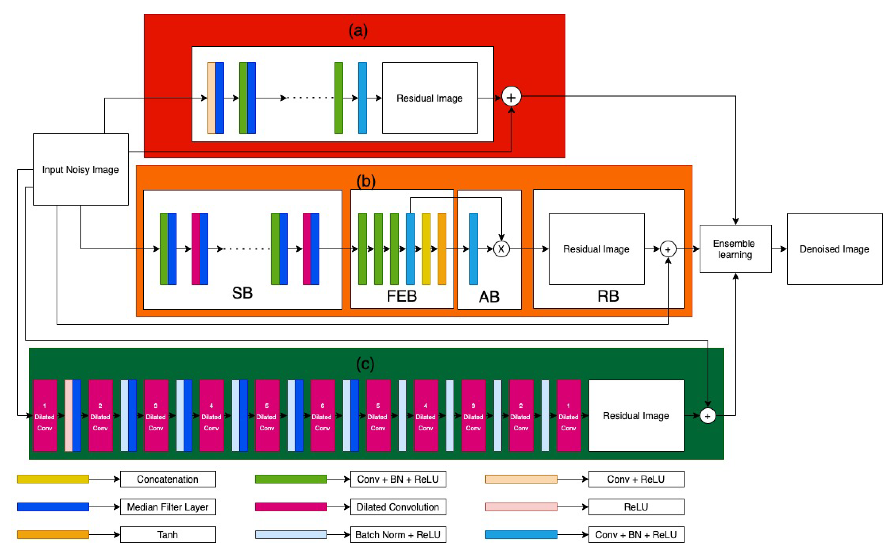
In this paper, we propose an ensemble of three image denoising models by using weighted mean of the output of the individual models, as shown in Figure 1. The models have been designed while keeping in mind that they should be able to span across a wide variety of images to efficiently denoise them. The architecture of individual models is described hereafter.
3.1. Attention-Guided CNN (ADNet)
There are 17 layers in total in ADNet, which are divided into four blocks, as shown in [4]. The first block is the Sparse Block (SB), the second block is the Feature Enhancement Block (FEB), the third is the Attention Block (AB), and the fourth block is the Reconstruction Block (RB). The SB contains 12 layers, it has two types of convolution—the dilated convolution and the standard convolution. The layers in the SB are of two types, the Dilated Convolution and the Normal convolution, both types being supported by Batch Normalization (BN) followed by the Relu activation function. The Dilated Conv (Dilated convolution) helps in increasing the size of receptive field without increasing the computation cost of the model. A dilated filter with dilation factor of a can be interpreted as a sparse filter of size .
The dilation rate of the dilated convolution used in SB is 8 and, also with each layer in the SB, we add a median filter layer, which is a traditional non-linear filter that replaces the pixel centred in a window with the median of the window, and helps in the efficient removal of impulse noise as mentioned in [26] by Liang et al. It is applied to each element of a feature channel in a moving window fashion. In case of each feature channel, we extract a set of patches of size ( or ) centred at each pixel. Subsequently, we find the median of the sequence formed by all elements in that patch and replace the elements with the median value.
The FEB consists of four layers and it aims to capture global and local features of the model to enhance the ability to express in image denoising. The global and local features that are used by the FEB are the input noisy image and the output of SB, respectively. The output from the FEB is passed on to the AB. The AB uses the current stage to guide the previous stage for learning the noise information, which is useful in terms of blind denoising and for extremely noisy images. The output of the AB is passed on as input to the RB, which uses a residual learning technique to reconstruct the clean image.
3.2. Feed Forward Denoising CNN (DnCNN)
The architecture of DnCNN is an end-to-end trainable deep CNN for Gaussian denoising and it adopts the residual learning strategy to remove the latent clean image from noisy observation, as reported in [6] by Zhang et al. The size of each convolutional filter is set to but without any pooling layers. Therefore, the receptive field of the architecture with depth of d should be . The total number of layers used in the model is 17 and each layer has Conv + BN + ReLU activation function. Along with it, median filter layers are used in the network, but only in the first half as the first half is used for removing the noise, whereas the second half is used to reconstruct the denoised image.
3.3. Deep CNN Denoiser Prior (IRCNN)
The architecture consists of 12 layers, which consist of three types of layers (i) Dilated Conv + ReLU, (ii) Dilated Conv + BN + ReLU, and (iii) Dilated Convolution which is used in the last layer as reported in [5] by Zhang et al. The dilation factors of dilated Conv layers from first to the last are set to 1, 2, 3, 4, 5, 6, 5, 4, 3, 2, and 1, respectively. The number of feature maps in each middle layer is set to 64. The use of batch normalization and residual learning helps to accelerate training. In particular, batch normalization and residual learning are helpful for Gaussian denoising, since they are beneficial to each other. Median filter layers are also added to the dilated Conv layer with a dilation rate of 6, so that it can help in increasing the denoising capability of the network.
3.4. Ensemble of Image Denoising Models
After training the individual image denoising models on the training dataset, we test them on images of the given testing dataset, and we then use the weighted average of the output of individual models to produce the final denoised image. As for the weights, we see the individual performance of the models on the images and use the corresponding results to decide the ratio in which the models are to be used for the ensemble. The ratio hence obtained is 2:3:6 for the ADNet, IRCNN, and DnCNN, respectively.
4. Experimental Results
4.1. Dataset
For evaluating our image denoising ensemble based model, we use the BSD500 dataset, which was proposed by Martin et al. in [29] and it can be downloaded from https://www2.eecs.berkeley.edu/Research/Projects/CS/vision/bsds/ BSD500 download (accessed on 27 March 2021), and the Set12 dataset [12], which is a collection of 12 widely used testing images available at https://www.researchgate.net/figure/12-images-from-Set12-dataset_fig11_338424598 Set12 download (accessed on 27 March 2021). We use 200 gray scale images of the BSD500 dataset and resize each image to for training our model. The BSD500 dataset is actually an extension of the BSDS300, in which the original 300 images are used for training and validation, and 200 fresh images, annotated by humans, are added for testing. We introduce additive white Gaussian noise in the images by setting the standard deviation of the Gaussian noise distribution to 15, 25, and 50, also known as noise levels. For training purpose, each image is converted into patches of size , which results in a total of 596 patches per image. The model is evaluated on the 200 testing images of the BSD500 dataset, whose results are illustrated in Table 1, and also on the 12 images from Set12 dataset whose results are illustrated in Table 2.
4.2. Hyperparameters
During the training phase, each model takes approximately two and a half hours to train. Hence, the entire ensemble model takes seven and a half hours to train. For the deep learning based models, through extensive experimentation with the dataset, we finally set the hyperparameters of the model as: learning rate = 0.001, number of epochs = 50, and steps per epoch = 1000. For testing, we use weighted average of the outputs of the three models. For the DnCNN + median layer model, we take th part of its output, for the IRCNN (dilation rate up to 6) + median layer model, we take th part of its output and for the ADNet (dilation rate = 8) + median layer model, we take th part of its output and then calculate the final output by adding all of them. We use PSNR (peak-signal-to-noise ratio) for evaluating the performance of the image denoising models. In case of the non-deep learning based methods, we use the scikit-image library [30] and, during application, we fine-tune the methods through extensive experimentation to obtain the best results. For TV-Chambolle [11], the denoising weight is set to 0.3 and the maximum number of iterations is set to 30. For Wavelet BayesShrink [10] and Wavelet VisuShrink [9] models, we use soft denoising and estimate the standard deviation of the noise using the method in [9].
4.3. Results
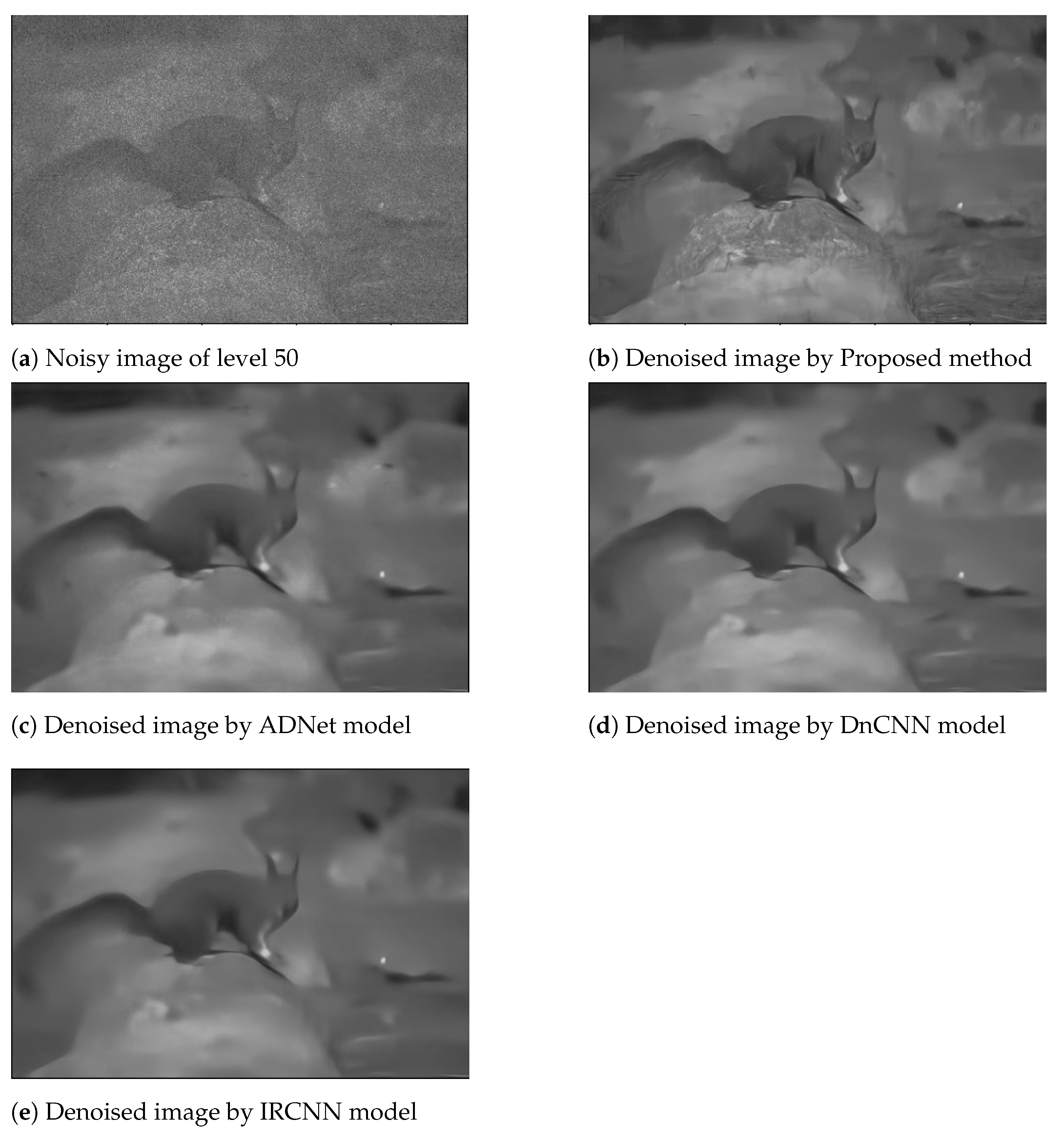
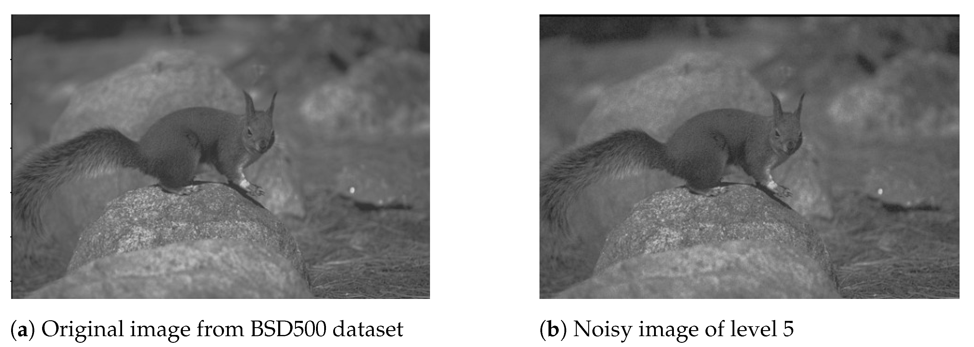
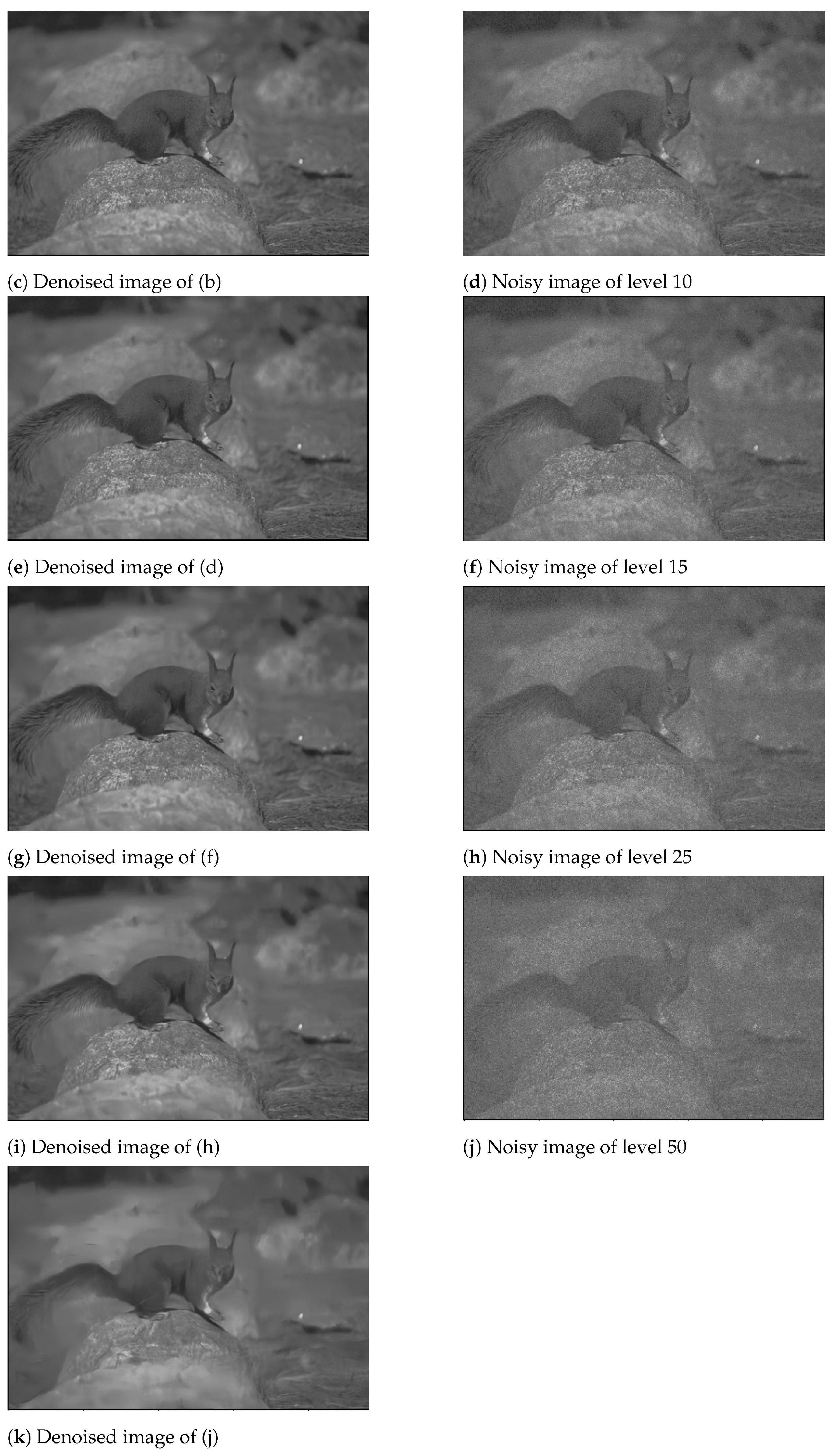
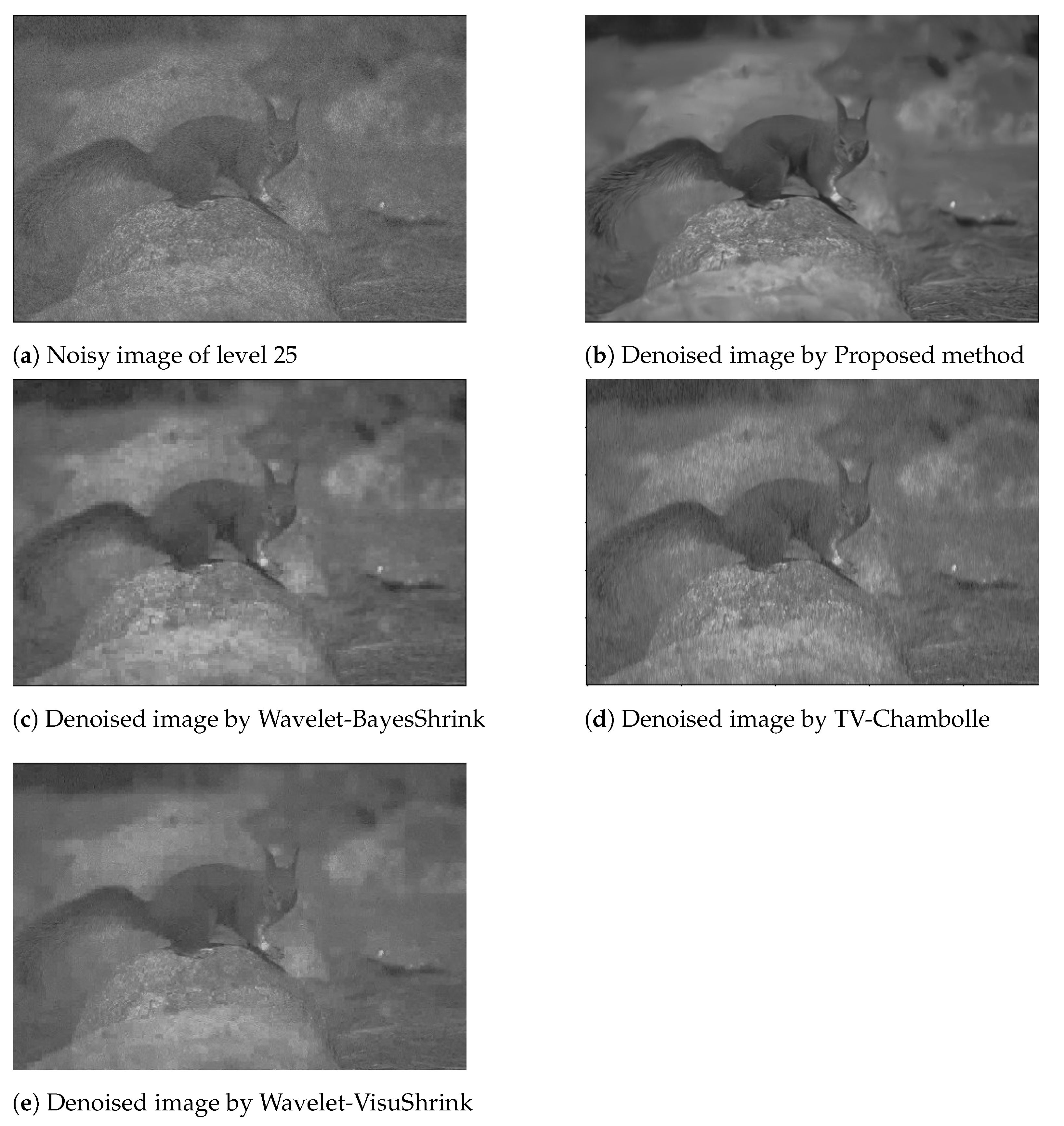
After thorough testing, as illustrated in Table 1 and Table 2, we note that the ensemble model outperforms all of the other model combinations and also some non-deep learning based models for the BSD500 dataset. For the Set12 dataset, we see that it provides extremely competitive results and outperforms other model combinations in most of the cases. When compared to non-deep learning based models, it completely outperforms them. Additionally, in Table 2, for noise level 15, out of the three non-deep learning models, the highest PSNR value is 23.54 dB, whereas the lowest PSNR value in the case of CNN based methods is 32.36 dB, which is 8.82 dB more than the best result of the non-deep learning models. Additionally, in the case of noise levels of 25 and 50, the CNN based methods perform better than the non-deep learning based methods. For the Set12 dataset, the trend is similar, as shown in Table 2. Thus, it is clear that the CNN based denoising models perform far better than the non deep learning based methods for the purpose in concern. Figure 2 shows the denoised images, as produced by DnCNN, IRCNN, ADNet, and our proposed ensemble model, for a noisy image of noise level 50. Various noisy versions of a single image with noise levels of 5, 10, 15, 25, and 50, along with their denoised versions, are shown in Figure 3. Additionally, we have shown the denoised results, for a noisy image of noise level 25, produced by the non-deep learning methods and the proposed ensemble method in Figure 4.
5. Conclusions
In this paper, we have proposed an ensemble of three deep learning models after suitable customizations for the purpose of image denoising. In the case of the first model, we use an ADNet with an increased dilation rate, along with median filter layers. In the case of the second model, we use a DnCNN with median filter layers and, for the third model, we use an IRCNN model with dilated convolutional layers and a dilation rate of 6 along with median filter layers. The final output image is a weighted average of the individual model’s output images. When comparing the performance of the proposed model to other state-of-the-art models, we observe that our model outperforms others when applied on the BSD500 dataset and, in the case of the Set12 dataset, our model outperforms most of the existing denoising models. In future, we would like to use our model for the denoising of images containing other types of noise, like salt-and-pepper noise and Poisson noise.
Author Contributions
Conceptualization, software, S.D.; methodology, formal analysis, S.D., R.B.; writing—original draft preparation, S.D., R.B., R.S.; validation, R.B., R.S. and F.S.; supervision, R.S., F.S.; project administration, F.S.; funding acquisition, F.S. All authors have read and agreed to the published version of the manuscript.
Funding
This research received no external funding.
Institutional Review Board Statement
Not applicable.
Informed Consent Statement
Not applicable.
Data Availability Statement
The code for our method is available here: https://github.com/subro608/Median-filter-aided-denoising. https://github.com/subro608/Median-filter-aided-denoising.
Acknowledgments
The authors would like to thank CMATER research laboratory of the Computer Science and Engineering Department, Jadavpur University, India for providing us the infrastructural support.
Conflicts of Interest
The authors declare no conflict of interest.
References
- Kortli, Y.; Jridi, M.; Al Falou, A.; Atri, M. Face recognition systems: A Survey. Sensors 2020, 20, 342. [Google Scholar] [CrossRef] [Green Version]
- Bhattacharya, R.; Malakar, S.; Ghosh, S.; Bhowmik, S.; Sarkar, R. Understanding contents of filled-in Bangla form images. Multimed. Tools Appl. 2020, 80, 3529–3570. [Google Scholar] [CrossRef]
- Yuan, Q.; Shen, H.; Li, T.; Li, Z.; Li, S.; Jiang, Y.; Xu, H.; Tan, W.; Yang, Q.; Wang, J.; et al. Deep learning in environmental remote sensing: Achievements and challenges. Remote Sens. Environ. 2020, 241, 111716. [Google Scholar] [CrossRef]
- Tian, C.; Xu, Y.; Li, Z.; Zuo, W.; Fei, L.; Liu, H. Attention-guided CNN for image denoising. Neural Netw. 2020, 124, 117–129. [Google Scholar] [CrossRef] [PubMed]
- Zhang, K.; Zuo, W.; Gu, S.; Zhang, L. Learning deep CNN denoiser prior for image restoration. In Proceedings of the IEEE Conference on Computer Vision and Pattern Recognition, Honolulu, HI, USA, 21–26 July 2017; pp. 3929–3938. [Google Scholar]
- Zhang, K.; Zuo, W.; Chen, Y.; Meng, D.; Zhang, L. Beyond a gaussian denoiser: Residual learning of deep cnn for image denoising. IEEE Trans. Image Process. 2017, 26, 3142–3155. [Google Scholar] [CrossRef] [Green Version]
- Pitas, I.; Venetsanopoulos, A. Nonlinear mean filters in image processing. IEEE Trans. Acoust. Speech Signal Process. 1986, 34, 573–584. [Google Scholar] [CrossRef]
- Hong, S.W.; Bao, P. An edge-preserving subband coding model based on non-adaptive and adaptive regularization. Image Vis. Comput. 2000, 18, 573–582. [Google Scholar] [CrossRef]
- Donoho, D.L.; Johnstone, J.M. Ideal spatial adaptation by wavelet shrinkage. Biometrika 1994, 81, 425–455. [Google Scholar] [CrossRef]
- Chang, S.G.; Yu, B.; Vetterli, M. Adaptive wavelet thresholding for image denoising and compression. IEEE Trans. Image Process. 2000, 9, 1532–1546. [Google Scholar] [CrossRef] [Green Version]
- Chambolle, A. An algorithm for total variation minimization and applications. J. Math. Imaging Vis. 2004, 20, 89–97. [Google Scholar]
- Dabov, K.; Foi, A.; Katkovnik, V.; Egiazarian, K. Image denoising by sparse 3-D transform-domain collaborative filtering. IEEE Trans. Image Process. 2007, 16, 2080–2095. [Google Scholar] [CrossRef]
- Schmidt, U.; Roth, S. Shrinkage fields for effective image restoration. In Proceedings of the IEEE Conference on Computer Vision and Pattern Recognition, Columbus, OH, USA, 23–28 June 2014; pp. 2774–2781. [Google Scholar]
- Chiang, Y.W.; Sullivan, B. Multi-frame image restoration using a neural network. In Proceedings of the IEEE 32nd Midwest Symposium on Circuits and Systems, Champaign, IL, USA, 14–16 August 1989; pp. 744–747. [Google Scholar]
- Zhou, Y.; Chellappa, R.; Jenkins, B. A novel approach to image restoration based on a neural network. In Proceedings of the International Conference on Neural Networks, San Diego, CA, USA, 21–24 June 1987. [Google Scholar]
- Mao, X.J.; Shen, C.; Yang, Y.B. Image restoration using convolutional auto-encoders with symmetric skip connections. arXiv 2016, arXiv:1606.08921. [Google Scholar]
- Zhang, Y.; Tian, Y.; Kong, Y.; Zhong, B.; Fu, Y. Residual dense network for image restoration. IEEE Trans. Pattern Anal. Mach. Intell. 2020. [Google Scholar] [CrossRef] [Green Version]
- Le Cun, Y.; Bottou, L.; Bengio, Y.; Haffner, P. Gradient-based learning applied to document recognition. Proc. IEEE 1998, 86, 2278–2324. [Google Scholar] [CrossRef] [Green Version]
- Krizhevsky, A.; Sutskever, I.; Hinton, G.E. Imagenet classification with deep convolutional neural networks. Adv. Neural Inf. Process. Syst. 2012, 25, 1097–1105. [Google Scholar] [CrossRef]
- Simonyan, K.; Zisserman, A. Very deep convolutional networks for large-scale image recognition. arXiv 2014, arXiv:1409.1556. [Google Scholar]
- Szegedy, C.; Liu, W.; Jia, Y.; Sermanet, P.; Reed, S.; Anguelov, D.; Erhan, D.; Vanhoucke, V.; Rabinovich, A. Going deeper with convolutions. In Proceedings of the IEEE Conference on Computer Vision and Pattern Recognition, Boston, MA, USA, 7–12 June 2015; Volume 1, p. 9. [Google Scholar]
- Lefkimmiatis, S. Non-local color image denoising with convolutional neural networks. In Proceedings of the IEEE Conference on Computer Vision and Pattern Recognition, Honolulu, HI, USA, 21–26 July 2017; pp. 3587–3596. [Google Scholar]
- Zhang, K.; Zuo, W.; Zhang, L. FFDNet: Toward a fast and flexible solution for CNN-based image denoising. IEEE Trans. Image Process. 2018, 27, 4608–4622. [Google Scholar] [CrossRef] [PubMed] [Green Version]
- Chen, J.; Chen, J.; Chao, H.; Yang, M. Image blind denoising with generative adversarial network based noise modeling. In Proceedings of the IEEE Conference on Computer Vision and Pattern Recognition, Salt Lake City, UT, USA, 18–23 June 2018; pp. 3155–3164. [Google Scholar]
- Guo, S.; Yan, Z.; Zhang, K.; Zuo, W.; Zhang, L. Toward convolutional blind denoising of real photographs. In Proceedings of the IEEE/CVF Conference on Computer Vision and Pattern Recognition, Long Beach, CA, USA, 15–20 June 2019; pp. 1712–1722. [Google Scholar]
- Liang, L.; Deng, S.; Gueguen, L.; Wei, M.; Wu, X.; Qin, J. Convolutional Neural Network with Median Layers for Denoising Salt-and-Pepper Contaminations. arXiv 2019, arXiv:1908.06452. [Google Scholar]
- Kirti, T.; Jitendra, K.; Ashok, S. Poisson noise reduction from X-ray images by region classification and response median filtering. Sādhanā 2017, 42, 855–863. [Google Scholar] [CrossRef] [Green Version]
- Islam, M.T.; Rahman, S.M.; Ahmad, M.O.; Swamy, M. Mixed Gaussian-impulse noise reduction from images using convolutional neural network. Signal Process. Image Commun. 2018, 68, 26–41. [Google Scholar] [CrossRef]
- Martin, D.; Fowlkes, C.; Tal, D.; Malik, J. A database of human segmented natural images and its application to evaluating segmentation algorithms and measuring ecological statistics. In Proceedings of the Eighth IEEE International Conference on Computer Vision. ICCV 2001, Vancouver, BC, Canada, 7–14 July 2001; Volume 2, pp. 416–423. [Google Scholar]
- Vvan der Walt, S.; Schönberger, J.L.; Nunez-Iglesias, J.; Boulogne, F.; Warner, J.D.; Yager, N.; Gouillart, E.; Yu, T. Scikitimage contributors. 2014. scikit-image: Image processing in python. PeerJ 2014, 2, e453. [Google Scholar] [CrossRef] [PubMed]
Figure 1.
Our proposed ensemble image denoising model. In the figure (a) denotes the improved Denoising CNNs (DnCNN) model, (b) represents the improved ADNet model, and (c) denotes the improved IRCNN model.
Figure 1.
Our proposed ensemble image denoising model. In the figure (a) denotes the improved Denoising CNNs (DnCNN) model, (b) represents the improved ADNet model, and (c) denotes the improved IRCNN model.

Figure 2.
Denoised images by DnCNN, IRCNN, ADNet, and Proposed ensemble methods.

Figure 3.
Noisy and denoised versions of the original image.


Figure 4.
Denoised images using non-deep learning models and Proposed ensemble method.


Table 1.
Average PSNR values of images predicted by the image denoising models on the images of BSD500 dataset.
Table 1.
Average PSNR values of images predicted by the image denoising models on the images of BSD500 dataset.
| Models | Noise Level 15 | Noise Level 25 | Noise Level 50 |
|---|---|---|---|
| TV-Chambolle [11] | 24.37 | 22.34 | 18.33 |
| Wavelet-VisuShrink [9] | 21.38 | 19.78 | 16.99 |
| Wavelet-BayesShrink [10] | 25.05 | 22.40 | 18.19 |
| ADNet model | 31.55 | 28.87 | 25.90 |
| IRCNN-model | 31.56 | 28.94 | 25.93 |
| DnCNN-model | 31.64 | 28.85 | 26.08 |
| ADNet(dilation rate = 8) + median layer | 31.63 | 29.12 | 25.98 |
| IRCNN-model (dilation upto 6) + median layer | 31.60 | 29.08 | 26.08 |
| DnCNN+ median layer | 31.66 | 29.08 | 26.10 |
| Ensemble-model | 31.73 | 29.20 | 26.20 |
Table 2.
Peak-signal-to-noise ratio (PSNR) values of images predicted by the image denoising models for different noise levels on Set12 image dataset.
Table 2.
Peak-signal-to-noise ratio (PSNR) values of images predicted by the image denoising models for different noise levels on Set12 image dataset.
| Denoising Models | 01. | 02. | 03. | 04. | 05. | 06. | 07. | 08. | 09. | 10. | 11. | 12. |
|---|---|---|---|---|---|---|---|---|---|---|---|---|
| Noise level of 15 | ||||||||||||
| TV-Chambolle [11] | 23.54 | 24.69 | 23.58 | 22.56 | 22.62 | 22.79 | 22.47 | 25.58 | 23.00 | 24.36 | 24.62 | 24.01 |
| Wavelet-VisuShrink [9] | 19.77 | 22.32 | 19.11 | 18.81 | 18.05 | 19.28 | 18.81 | 21.94 | 19.82 | 20.95 | 21.20 | 20.93. |
| Wavelet-BayesShrink [10] | 23.40 | 26.07 | 23.76 | 23.10 | 22.82 | 23.20 | 23.15 | 26.21 | 23.19 | 24.75 | 25.16 | 24.56. |
| ADNet | 32.36 | 34.46 | 33.08 | 31.80 | 32.64 | 31.58 | 31.73 | 34.12 | 31.56 | 32.16 | 32.20 | 32.12 |
| IRCNN-model | 32.40 | 34.44 | 33.07 | 31.73 | 32.65 | 31.55 | 31.75 | 34.14 | 31.82 | 32.20 | 32.21 | 32.12 |
| DnCNN-model | 32.56 | 34.66 | 33.24 | 32.00 | 32.85 | 31.66 | 31.80 | 34.28 | 32.07 | 32.28 | 32.30 | 32.25 |
| ADNet + median layer | 32.45 | 34.60 | 33.11 | 31.87 | 32.70 | 31.62 | 31.70 | 34.22 | 31.73 | 32.23 | 32.25 | 32.22 |
| IRCNN-model + median layer | 32.41 | 34.52 | 33.03 | 31.70 | 32.60 | 31.55 | 31.70 | 34.18 | 31.80 | 32.21 | 32.20 | 32.17 |
| DnCNN + median layer | 32.56 | 34.75 | 33.24 | 31.93 | 32.66 | 31.67 | 31.75 | 34.31 | 32.11 | 32.26 | 32.31 | 32.27 |
| Ensemble method | 32.60 | 34.78 | 33.27 | 32.00 | 32.81 | 31.71 | 31.84 | 34.35 | 32.13 | 32.32 | 32.34 | 32.30 |
| Noise level of 25 | ||||||||||||
| TV-Chambolle [11] | 19.89 | 20.72 | 20.20 | 19.75 | 19.77 | 19.96 | 19.32 | 21.10 | 20.14 | 20.54 | 20.85 | 20.48. |
| Wavelet-VisuShrink [9] | 18.11 | 20.66 | 17.60 | 17.49 | 16.34 | 18.04 | 16.95 | 20.14 | 18.43 | 19.59 | 19.74 | 19.67. |
| Wavelet-BayesShrink [10] | 20.91 | 23.78 | 21.07 | 20.94 | 20.52 | 20.90 | 20.30 | 24.12 | 21.44 | 22.75 | 23.25 | 22.62. |
| ADNet | 29.87 | 32.36 | 30.50 | 29.03 | 29.84 | 28.90 | 29.14 | 31.80 | 29.07 | 29.81 | 29.71 | 29.68 |
| IRCNN-model | 29.77 | 32.33 | 30.46 | 28.93 | 29.75 | 28.83 | 29.20 | 31.85 | 29.00 | 29.84 | 29.78 | 29.63 |
| DnCNN-model | 30.05 | 32.70 | 30.77 | 29.15 | 30.03 | 29.02 | 29.28 | 32.07 | 29.21 | 29.98 | 29.90 | 29.84 |
| ADNet + median layer | 30.04 | 32.60 | 30.64 | 29.26 | 29.98 | 28.98 | 29.30 | 32.04 | 29.14 | 30.00 | 29.90 | 29.82 |
| IRCNN-model + median layer | 29.98 | 32.57 | 30.65 | 29.13 | 29.90 | 28.90 | 29.22 | 32.05 | 28.70 | 29.92 | 29.86 | 29.81 |
| DnCNN + median layer | 30.03 | 32.73 | 30.76 | 29.16 | 29.47 | 29.04 | 28.81 | 32.09 | 29.35 | 30.02 | 29.93 | 29.88 |
| Ensemble method | 30.15 | 32.80 | 30.80 | 29.31 | 29.94 | 29.09 | 29.23 | 32.17 | 29.45 | 30.10 | 29.98 | 30.00 |
| Noise level of 50 | ||||||||||||
| TV-Chambolle [11] | 14.59 | 15.21 | 14.98 | 14.73 | 14.83 | 14.67 | 14.38 | 15.27 | 14.93 | 15.13 | 15.14 | 15.10. |
| Wavelet-VisuShrink [9] | 16.04 | 18.40 | 15.79 | 15.63 | 14.73 | 15.73 | 14.67 | 17.65 | 16.18 | 17.68 | 17.42 | 17.85. |
| Wavelet-BayesShrink [10] | 17.40 | 20.02 | 18.02 | 17.30 | 17.07 | 17.05 | 16.56 | 20.12 | 18.38 | 19.50 | 19.61 | 19.71. |
| ADNet | 26.87 | 29.37 | 27.03 | 25.38 | 26.27 | 25.63 | 25.97 | 28.74 | 25.43 | 26.89 | 26.87 | 26.51 |
| IRCNN-model | 26.90 | 29.51 | 27.17 | 25.40 | 26.43 | 25.68 | 26.08 | 29.00 | 25.58 | 26.98 | 27.01 | 26.56 |
| DnCNN-model | 27.10 | 29.56 | 27.23 | 25.47 | 26.47 | 25.72 | 26.24 | 28.97 | 25.53 | 27.03 | 27.02 | 26.67 |
| ADNet + median layer | 26.85 | 29.45 | 27.04 | 25.41 | 26.38 | 25.56 | 26.00 | 28.86 | 25.57 | 26.90 | 25.90 | 26.64 |
| IRCNN-model + median layer | 26.93 | 29.55 | 27.22 | 25.47 | 26.37 | 25.76 | 26.00 | 29.07 | 25.78 | 27.08 | 27.05 | 26.74 |
| DnCNN + median layer | 27.11 | 29.65 | 27.20 | 25.47 | 26.47 | 25.72 | 26.16 | 28.97 | 25.54 | 27.05 | 27.02 | 26.70 |
| Ensemble method | 27.17 | 29.80 | 27.30 | 25.56 | 26.60 | 25.78 | 26.26 | 29.11 | 25.73 | 27.12 | 27.09 | 26.81 |
| End of Table | ||||||||||||
Publisher’s Note: MDPI stays neutral with regard to jurisdictional claims in published maps and institutional affiliations. |
© 2021 by the authors. Licensee MDPI, Basel, Switzerland. This article is an open access article distributed under the terms and conditions of the Creative Commons Attribution (CC BY) license (http://creativecommons.org/licenses/by/4.0/).
Share and Cite
MDPI and ACS Style
Dey, S.; Bhattacharya, R.; Schwenker, F.; Sarkar, R. Median Filter Aided CNN Based Image Denoising: An Ensemble Approach. Algorithms 2021, 14, 109. https://0-doi-org.brum.beds.ac.uk/10.3390/a14040109
AMA Style
Dey S, Bhattacharya R, Schwenker F, Sarkar R. Median Filter Aided CNN Based Image Denoising: An Ensemble Approach. Algorithms. 2021; 14(4):109. https://0-doi-org.brum.beds.ac.uk/10.3390/a14040109
Chicago/Turabian StyleDey, Subhrajit, Rajdeep Bhattacharya, Friedhelm Schwenker, and Ram Sarkar. 2021. "Median Filter Aided CNN Based Image Denoising: An Ensemble Approach" Algorithms 14, no. 4: 109. https://0-doi-org.brum.beds.ac.uk/10.3390/a14040109
Note that from the first issue of 2016, this journal uses article numbers instead of page numbers. See further details here.