An Effective Decomposition-Based Stochastic Algorithm for Solving the Permutation Flow-Shop Scheduling Problem

Abstract

This paper presents an effective stochastic algorithm that embeds a large neighborhood decomposition technique into a variable neighborhood search for solving the permutation flow-shop scheduling problem. The algorithm first constructs a permutation as a seed using a recursive application of the extended two-machine problem. In this method, the jobs are recursively decomposed into two separate groups, and, for each group, an optimal permutation is calculated based on the extended two-machine problem. Then the overall permutation, which is obtained by integrating the sub-solutions, is improved through the application of a variable neighborhood search technique. The same as the first technique, this one is also based on the decomposition paradigm and can find an optimal arrangement for a subset of jobs. In the employed large neighborhood search, the concept of the critical path has been used to help the decomposition process avoid unfruitful computation and arrange only promising contiguous parts of the permutation. In this fashion, the algorithm leaves those parts of the permutation which already have high-quality arrangements and concentrates on modifying other parts. The results of computational experiments on the benchmark instances indicate the procedure works effectively, demonstrating that solutions, in a very short distance of the best-known solutions, are calculated within seconds on a typical personal computer. In terms of the required running time to reach a high-quality solution, the procedure outperforms some well-known metaheuristic algorithms in the literature.

1. Introduction

The endeavor of developing a suitable neighborhood scheme is a key factor in the success of any local search algorithm. The reason is that the critical role the size of the neighborhood plays in striking a balance between the effectiveness and computational time [1,2]. For striking such a balance in solving the permutation flow-shop scheduling problem, this paper presents a two-level decomposition-based, variable neighborhood search stochastic algorithm that embeds a large neighborhood scheme into a small one.

The algorithm, called Refining Decomposition-based Integrated Search (RDIS), refines a solution obtained by its small neighborhood search through its large neighborhood search, and uses the notion of decomposition in the two levels of (i) producing an initial solution, and (ii) performing large neighborhood search on the initial solution. Both neighborhood schemes employed are k-exchange [3].

The k-exchange schemes, as the most common types of neighborhood schemes, consider two candidate solutions as neighbors if they differ in at most k solution elements [3]. It is clear that larger neighborhood schemes contain more and potentially better candidate solutions but this increases the neighborhood size of these schemes exponentially with k [2]. In effect, when k is as large as the size of the problem, the corresponding neighborhood scheme makes local optimal solutions global optimal; however, because of their impracticality, these kinds of neighborhood schemes are not used in practice. On the other hand, smaller values of k require lower computational time at the cost of generating fewer candidate solutions [1,3].

In combing small and large neighborhood schemes, the RDIS has three synergetic characteristics of (i) generating an initial solution with a construction method that has been built upon the concept of decomposition of jobs and the extended two-machine solution strategy, (ii) improving the initial solution with a small neighborhood search, and (iii) enhancing the result produced by the small-neighborhood search with a large neighborhood search which has been built based on a decomposition technique.

The construction method for generating initial solutions is based on the recursive application of the extended 2-machine problem [4], described in Section 2. Aimed at generating high-quality solutions, and inspired by the famous two-machine problem [4], this recursive algorithm repeatedly decomposes the jobs and finds the best permutation for the decomposed jobs, with the goal of improving the quality of initial solutions.

Although the employed large neighborhood search, the same as the engaged construction method, is based on decomposition, it performs decomposition in an iterative manner, and not recursively. This iterative decomposition technique starts with the top k jobs in the permutation and ends with the k bottom jobs, ignoring any unfruitful contiguous parts in the middle. In each round, it also keeps the result of calculations in memory to prevent any repeat of calculations in further rounds. In optimizing small chunks, this effective use of memory makes the optimization process as fast as simple decoding of a permutation to a solution. The main contributions of this paper are outlined in the following:

• The effective embedding of a large neighborhood decomposition technique into a variable neighborhood search for the permutation flow-shop scheduling problem;
• Efficient decomposition of the main problem into subproblems, and finding optimal permutations for those smaller subproblems; and
• Employing the concept of the critical path, as described in Section 4, in the employed large neighborhood search.

The paper is structured as follows. In Section 2, the related work is discussed, and Section 3 presents the formulation of the permutation flow-shop scheduling problem. Section 4 presents the RDIS and provides a stepwise description of the corresponding algorithm. In Section 5, the results of computational experiments are discussed. The concluding remarks, as well as the suggestions for the further enhancement of the stochastic algorithm, are discussed in Section 6.

2. Related Work

In manufacturing systems, scheduling is about the allocation of resources to operations over time to somehow optimize the efficiency of the corresponding system. Quite interestingly, because of their complexity, scheduling problems have been among the first categories of problems that have promoted the development of the notion of NP-completeness [5].

The Flow-shop Scheduling Problem (FSP), in which jobs should pass all machines in the same order, is one of the easy-to-state but hard-to-solve problems in scheduling. Because of these contrasting features, the FSP is one of the first problems in scheduling which captured the attention of pioneers in scheduling [4,6], and later became an attractive topic for a significant number of researchers.

Interestingly, one of the most elegant procedures in the area of algorithmic design is an efficient exact algorithm [4] that has been presented for the two special cases of this problem, which are a two-machine problem and a restricted case of the three-machine problem. Although this algorithm has been extended [6,7] to tackle some less restricted cases of the three-machine problem, it has never been extended to solve problems with a larger number of machines to optimality.

Several variations and extensions of the FSP, with multiple objective function criteria, have been studied in the literature [8,9,10]. Among the variants of the FSP, the Permutation Flow-shop Scheduling Problem (PFSP), in which jobs have the same sequence on all machines, plays a key role. The PFSP best suits multi-stage production systems in which conveyor belts are used to perform material handling between machines. Both the FSP and the PFSP have shown to be NP-Hard [11,12]. An interesting variant of the PFSP is the distributed permutation flow shop scheduling problem (DPFSP) which has been studied in [13], and, in [14], energy consumption is considered as one of its multi-objective criteria. The rest of this section briefly surveys the related literature with a focus on the PFSP.

Extensive literature surveys on the early efficient algorithms presented for the FSP can be found in [15,16]. A more recent review and classification of heuristics for the PFSP has been presented in [17]. In the proposed framework of [17], heuristics are analyzed in the three phases of (i) index development, (ii) solution construction and (iii) solution improvement. In the following, some related work is briefly reviewed.

The most related method is Jonson’s method that because of the complete dependence of the RDIS on it, this method will be described as part of the RDIS in Section 4. The Palmer method developed in [18] can be considered as another related work. The author has not provided any reference to Johnson’s paper but has mentioned that the rationale behind the development of the procedure is to minimize the makespan based on the notion of the lower bound of the single machine problem, which is obtained by the head time plus its total processing times plus its tail time. It is these heads and tails that the Palmer algorithm tries to minimize.

Based on advancing Palmer’s index method, an algorithm has been presented in [19] which works based on a slope matching mechanism. First, assuming that only one job exists, the starting time and ending time of each job on each machine is calculated and, by running the regression, a starting slope and an ending slope are calculated for each job.

The first method, with which they have compared their two techniques, is the method presented in [20], that finds the actual slope of jobs. For calculating this actual slope, simply the regression is run for each job.

The other method that they have compared with their two methods is the method based on the priority presented by [21], and obtained based on Johnson’s rule.

In comparing these four methods with one another, they found the following ranking (i) TSP-approximation, (ii) slope-matching mechanism, (iii) Gupta’s method, and (iv) Palmer’s method. These ranking criteria can be used as the basis of any construction method.

As another example, in [22] a heuristic algorithm for n-job m-machine sequencing problem has been presented that, based on the two-machine problem, builds a sequence by decomposing total processing times into three parts.

Among other effective heuristics developed for the permutation flow-shop problem, TB [23], SPIRIT [24], FSHOPH [25], NEH [26], and NEHLJP1 [27] can be mentioned. It is worth noting that NEH is one of the earliest effective heuristics and it is incorporated in many other metaheuristics. For instance, an iterated greedy algorithm is presented in [28], in which a solution is improved through repeated removal and re-insertion of the jobs, from a given solution, using the NEH heuristic.

Some effective metaheuristics developed are Ogbu and Smith’s simulated annealing [29], Taillard’s tabu search [30], Nowicki and Smutnicki’s fast tabu search [31], Reeves’s genetic algorithm [32], Nowicki and Smutnicki’s scatter search [33], Iyer and Saxena’s genetic algorithm [34], Yagmahan and Yenisey’s ant colony algorithm [35], Lian et al.’s particle swarm algorithm [36], artificial bee colony algorithm of [37], Discrete differential evolution algorithm of [38], algebraic decomposition-based evolutionary algorithm of [8], and re-blocking adjustable memetic Procedure (RAMP) of [39]. A comprehensive review and comparison of heuristics and metaheuristics for the PFSP can found in [40].

3. Problem Formulation

Assuming that there are n jobs and m machines, and that all jobs require to be processed on machines 1, 2, 3,..., and m, one after another, the PFSP is aimed at finding a permutation $\pi$ of jobs, identical for all machines, that minimizes the completion time of the last job on the last machine, referred to as makespan.

Given a permutation $\pi =({\pi }_1,{\pi }_2,\cdots ,{\pi }_n)$, in which ${\pi }_k$ shows the number of job in the sequence of jobs, and denoting the processing time of job j on machine i, as t_ji, the makespan of the problem can be calculated by rearranging the jobs based on $\pi$. In effect, by denoting the earliest completion time of job ${\pi }_k$ on the machine i as $c_{ki}$, the value of $c_{nm}$ shows the exact amount of makespan. Hence, the objective can be stated as finding a permutation ${\pi }^{\ast }$ over the set of all permutations, $\Pi$, so that $c_{nm}$ is minimized. A simple formulation of the PFSP, based on the formulation presented in [41] is as follows.

$$\begin{array}{ccc}\hfill \underset{\pi \in \Pi }{min}{c}_{nm}& \hfill & \end{array}$$

(1)

where,

$$\begin{array}{cccc}\hfill c_{11}& =t_{{\pi }_1,1}\hfill & \hfill & \end{array}$$

(2)

$$\begin{array}{cccc}\hfill c_{1i}& =c_{1,i-1}+t_{{\pi }_1,i}\hspace{1em}\hspace{1em}\hspace{1em}\hspace{1em}\hspace{1em}\hfill & \hfill i=2,3,\cdots ,m& \end{array}$$

(3)

$$\begin{array}{cccc}\hfill c_{k1}& =c_{k-1,1}+t_{{\pi }_k,1}\hfill & \hfill k=2,3,\cdots ,n& \\ \hfill c_{ki}& =max(c_{k,i-1},c_{k-1,i})+t_{{\pi }_k,i}\hfill & \hfill i=2,3,\cdots ,m\end{array}$$

(4)

$$\begin{array}{ccc}\hfill & \hfill & \hfill k=2,3,\cdots ,n\end{array}$$

(5)

It is worth noting that Formulas (2)–(5) also shows how, for a given permutation, the makespan can be calculated in $O\left(nm\right)$.

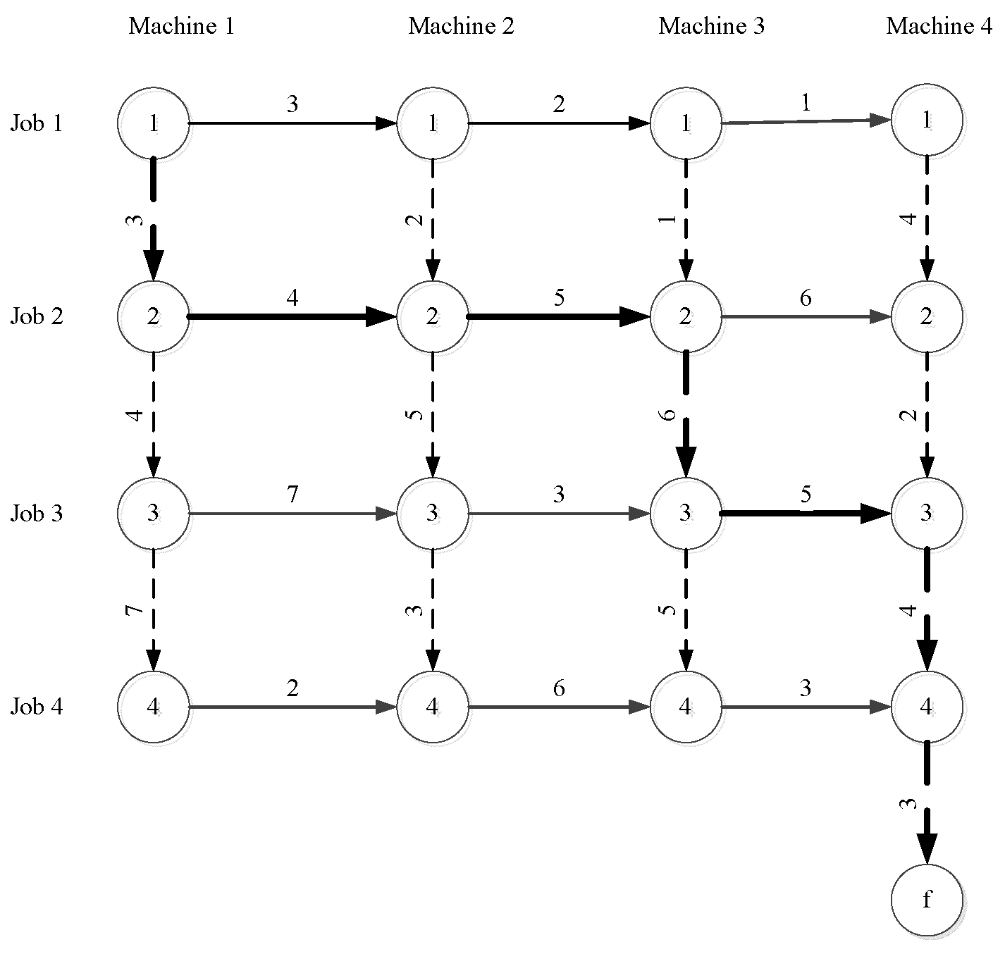
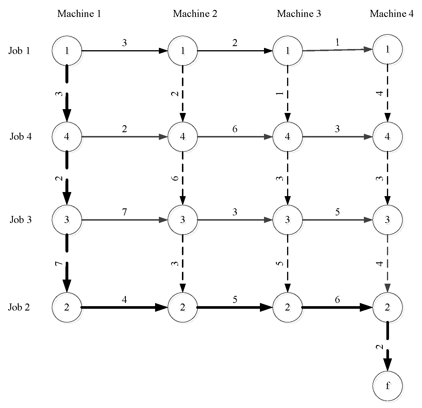
Figure 1 shows a sample 4-Job 4-Machine PFSP problem, with the permutation ${\pi }_1=(1,2,3,4)$ of jobs leading to the solution value of 30. The arrows originating from each circle in Figure 1, show the corresponding processing time of the corresponding job on the corresponding machine and the sum of processing times on the bold arrows indicates the makespan. Figure 2 shows how by changing the order of ${\pi }_1=(1,2,3,4)$ to ${\pi }_2=(1,4,3,2)$, the makespan has changed to 29, which is the optimal solution.

4. RDIS

A key justification for the design of the RDIS is an effective integration of decomposition, converting a non-tractable problem into tractable subproblems, with variable neighborhood search techniques, synergetically striking a balance between diversification and intensification elements of the algorithm.

Starting with the notion of decomposition, the RDIS works in the two levels of constructing an initial solution, and improving this solution through local searches. For this purpose, it first employs the recursive application of the extended two-machine problem as a seed-construction technique and constructs an initial permutation as a seed. This construction technique recursively decomposes the jobs into two groups and calculates the optimal solutions of each group based on the extended two-machine problem.

After such an initial seed is constructed, a variable neighborhood search is activated. This variable neighborhood search consists of two local searches, one with the small neighborhood and the other with the large neighborhood. The large neighborhood local search uses a decomposition technique for finding an optimal arrangement for different subsets of jobs. In effect, both the seed construction technique and the employed large neighborhood search work are based on the notion of decomposition.

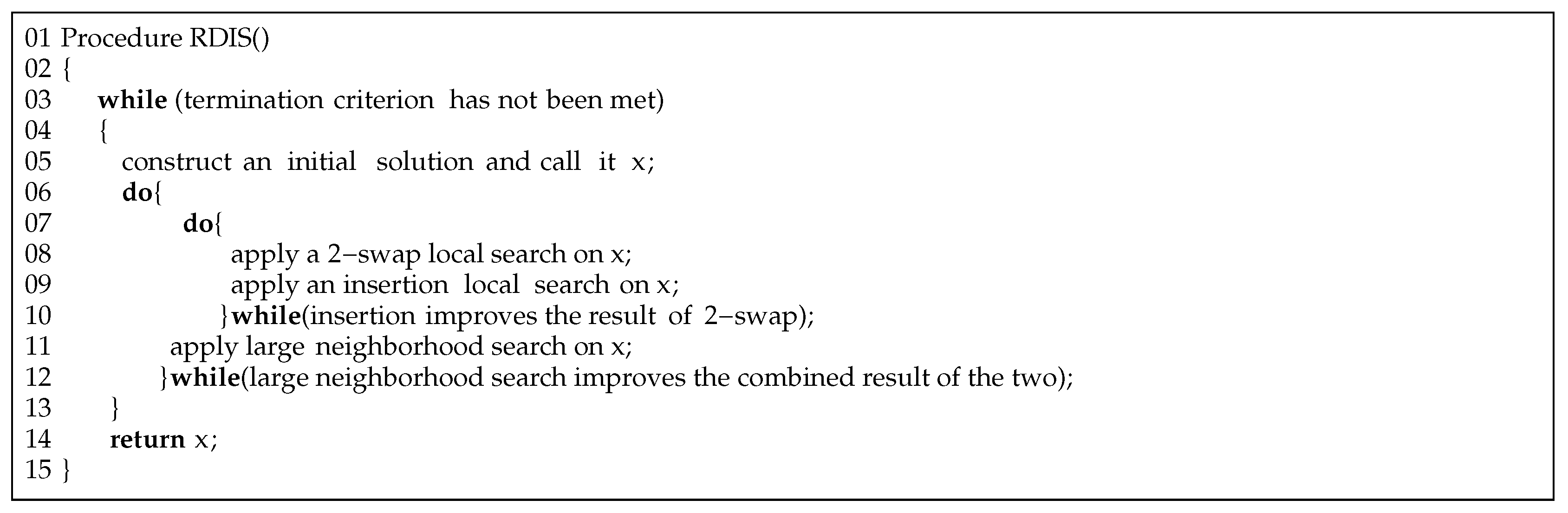
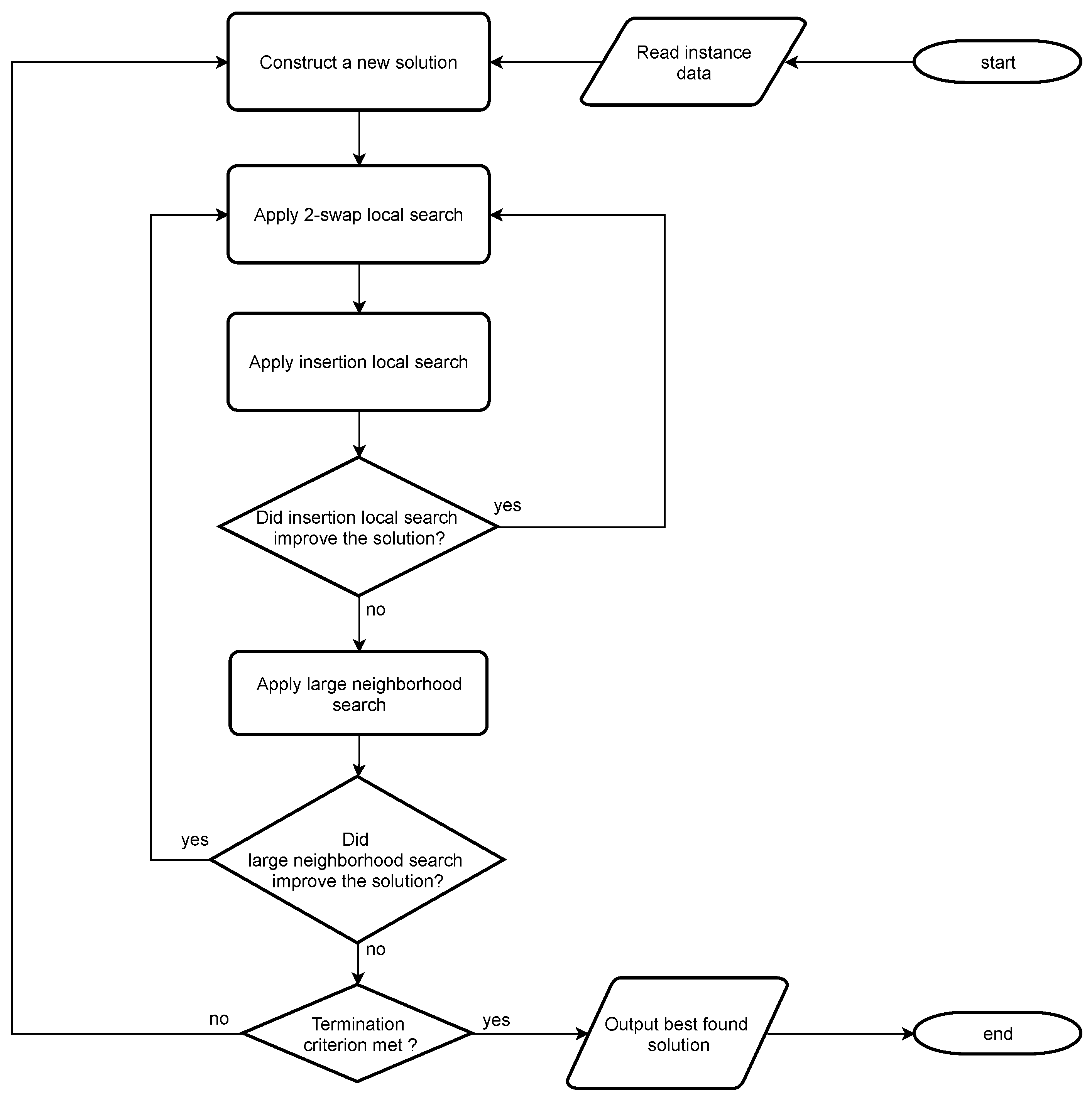
The small neighborhood search component uses both the insertion and swapping operations as the basis of its moves. In both the small and large neighborhood searches, the concept of the critical path plays a crucial role in avoiding unfruitful changes. Whereas in the small neighborhood, the critical path is used to avoid unfruitful swaps or interchanges, in the large neighborhood search, it is used to re-arrange only promising contiguous parts of the permutation, leaving those parts whose re-arrangement is not beneficial. Figure 3 shows the c-type pseudocode of the RDIS, and Figure 4 shows the flowchart of the key steps of the RDIS.

In describing different components of this pseudocode, first, we describe the way in which the seed-construction technique uses decomposition to create the initial solutions. For creating this technique, we have modified the Johnson algorithm [4] and called the result the Recursive-Johnson Procedure (RJP). For tackling any PFSP problem, the RJP decomposes it into smaller problems and continues this in different rounds until the decomposed problem includes only one job or one machine.

The decomposition process in the RJP proceeds in several consecutive rounds. In the first round, the number of columns (machines) of the decomposed problems is divided into two equal parts, with the first machines comprising the first part and the last machines comprising the second part. All machines located in the first part comprise auxiliary machine 1, and those in the second part comprise auxiliary machine 2.

Then the corresponding two-machine problem is solved with Johnson’s algorithm and a permutation for the given jobs is determined. This permutation is only a preliminary one and the goal of further rounds is to further improve this permutation. Because of the recursive nature of the algorithm, further rounds are similar to the first round and their only difference is that they operate on a portion of jobs.

The employed large neighborhood search decomposes the problem into several distinct parts and optimizes each part separately. Based on a technique initially proposed in [30], two forward and backward matrixes simultaneously help the optimization cost to decrease.

Whereas in the forward matrix the distance of each operation from the first performed operation is presented, in the backward matrix, the distance of each operation from the final performed operation is provided. Moreover, the preliminary evaluation renders many of these combinations unnecessary. Because of using two forward and backward matrixes, when the positions of two jobs are not far from one another in the permutation, the evaluation of their swap can be performed very fast.

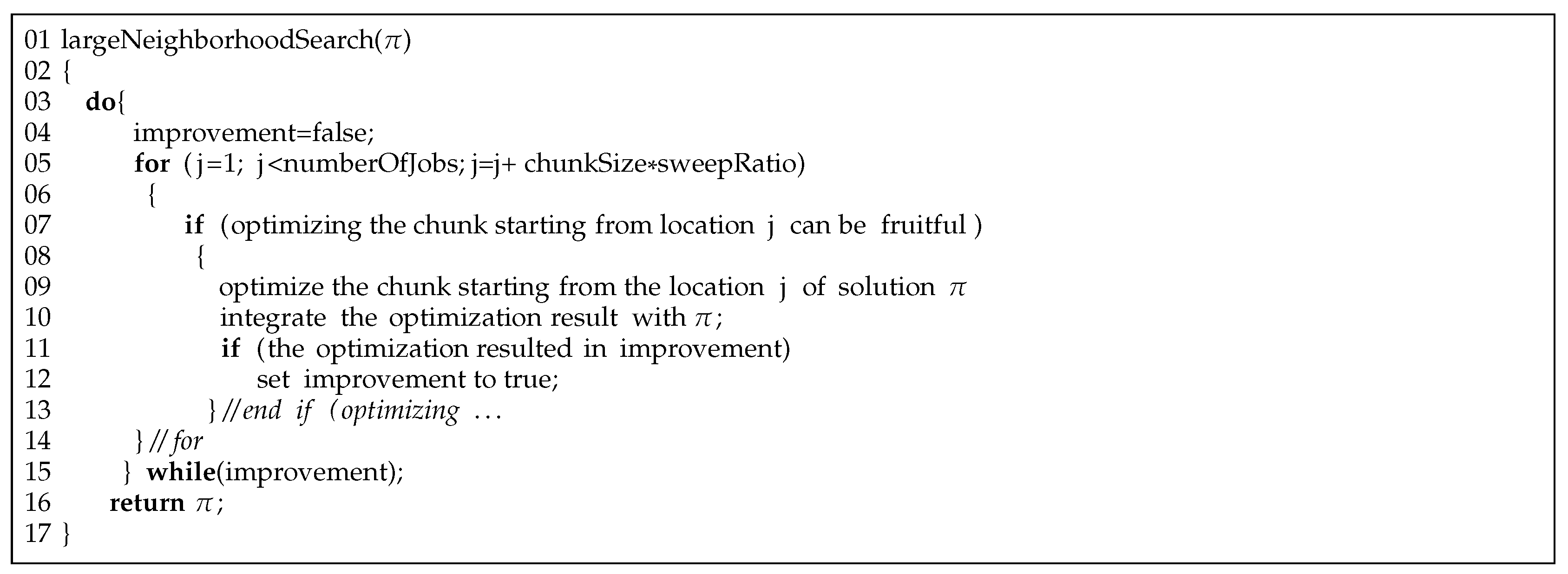
The solutions provided by the RJP undergo both small and large neighborhood searches. As is seen in the pseudocode presented in Figure 3, the large neighborhood search is called at line 11. The pseudocode presented in Figure 5 describes how this large neighborhood search operates. As is seen in this pseudocode, the main loop starts at line 3 and is aimed at improving the given solution, shown with permutation $\pi$, through modifying different parts of this permutation.

The substrings selected for modification are called chunk and all have the same size of chunkSize. For the purpose of modification, a subproblem of the given problem is solved to optimality through evaluating all possible ordering of jobs in a given chunk, keeping other jobs fixed in their current positions. In particular, it is line 9 of the pseudocode that calculates the makespan values of all chunkSize! permutations. For instance, if the value of chunkSize is 6, line 9 has to evaluate 6! = 720, different permutations to find the optimal one.

As is shown in line 5, the number of chunks to be optimized for a given solution is controlled through a parameter named sweepRatio, which is in the range between 0 and 1. For instance, setting sweepRatio to 0.5 and chunkSize to 6 the first chunk, which starts from position 1 and ends in position 6, to be optimized and then the starting position for the next chunk to be set to $(1+6\ast 0.5)=4$.

In other words, around 50% of jobs for the optimized chunk are fixed and the remaining jobs appear in the first half of the next chunk to be optimized. After re-arranging the chunk starting at position 4, through the employed optimization process, and ending at position 9, positions 4, 5, and 6 are fixed and the next chunk starting from position 7 and ending in position 12 is selected for being re-arranged.

Fixing half of the re-arranged jobs in a chunk and carrying the other half with the next chunk continues until a chunk is selected whose ending point is the last position in the permutation, signaling the end of a cycle. As indicated in lines 3 and 15 of the pseudocode, a new cycle can again resume from position 1 if the current cycle has been able to improve the solution.

The quality of the obtained solutions depends on the values of chunkSize and sweepRatio. Whereas increasing the value of sweepRatio leads to increasing the exploration power and reduces computation time, its decreasing can produce better solutions at the expense of higher computation time. Since optimizing a chunk is involved with evaluating chunkSize! permutations, the execution time is highly dependent on the chunk size.

This implies that a combination of selecting a proper value for this parameter and a mechanism for the recognition of unfruitful chunks can greatly improve the efficiency of the stochastic algorithm. Values between 6 and 9 for chunkSize can lead to improving solution quality, without increasing execution time significantly.

With respect to having a necessary mechanism for the recognition of unfruitful chunks, line 7 detects such chunks based on the critical path properties of the current solution. This is done based on the fact that if all of the critical operations in a chunk belong to the same machine, optimizing such a chunk cannot reduce the makespan, and therefore the chunk can be skipped. In other words, regardless of the order of jobs in such an unfruitful chunk, the previous critical path persists in the new solution and this makes any decrease in the makespan impossible.

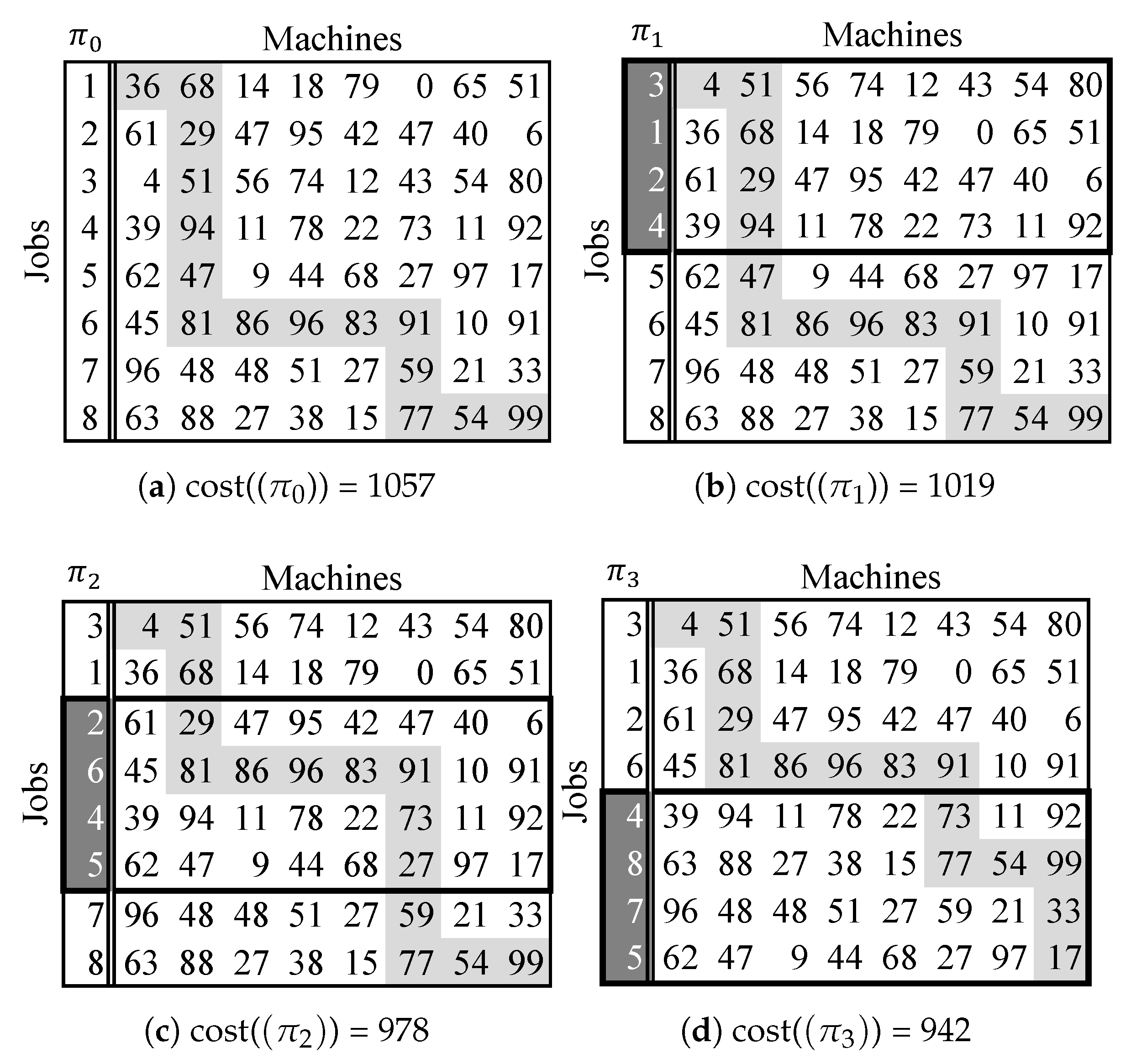
Setting the values of chunkSize and sweepRatio to 4 and 0.5, respectively, Figure 6 illustrates how the application of just one cycle of the steps presented in the pseudocode leads to improving an initial solution for a sample 8-jobs 8-machines instance from 1057 to 942. In this instance, the processing times of operations have been selected as integers between 0 and 100 with a uniform distribution.

As is seen in the figure, each solution has been shown with a matrix, in which the permutation of jobs has been represented in its first column. In each matrix, the critical operations corresponding to the solution are highlighted and its makespan, which is equal to the sum of the highlighted processing times, has also been shown. Figure 6a shows the initial solution, ${\pi }_0=\{1,2,3,4,5,6,7,8\}$ with the cost of 1057.

In Figure 6b, the first chunk $[1,2,3,4]$ is optimized and is changed to $[3,1,2,4]$. This alone reduces the makespan by 38 units and changes it to 1019. Since the sweepRatio is 0.5, the next chunk to be optimized starts from the 3rd row and is $[2,4,5,6]$ which is optimized to $[2,6,5,4]$, shown in Figure 6c.

This procedure continues accordingly and optimizes all corresponding chunks. As mentioned, Figure 6 shows the result of applying the main loop of the psedudocode just for one cycle and as lines 3, 4 and 15 of the pseudocode show, in general, the optimization of chunks continues for consecutive cycles until no improvement occurs in a cycle.

5. Computational Experiments

The RDIS has been implemented in C++ and compiled via the Visual C++ compiler on a PC with 2.2 GHz speed. Before testing the algorithm on the benchmark instances, the parameters of the construction and large neighborhood components have been set. With respect to the construction component, tthe algorithm has two parameters, namely NRepeats and SwapProb, indicating the frequency and the probability of performing swap moves in the RJP method. Based on the preliminary experiments, we observed that setting NRepeats and SwapProb to 1 and 0.4, respectively, yields the best results by providing a balance between the quality and diversity of the initial solutions generated by the construction component.

With respect to the large neighborhood component, the RDIS has also two parameters, namely ChunkSize, and SweepRatio. Setting ChunkSize to a small value (≤5) will increase the speed of the procedure at the expense of lower solution quality. On the other hand, setting ChunkSize to any value larger than 10 will dramatically increase the running time. Moreover, the computational experiments show that setting the value of SweepRatio close to 1 or 0 degrades the performance. Due to these observations, and based on further preliminary experiments, ChunkSize and SweepRatio have been set to 7 and 0.3, respectively.

We have employed Taillard’s repository of benchmark instances [42], available on the website supported by the University of Applied Sciences of Western Switzerland, to test the performance of the RDIS. In this repository, as many as 120 instances exist, and all of these instances have been extracted for the RDIS to be tested on. These instances are in 12 classes, with 10 instances existing in each class. The number of jobs and machines of these instances are in the range 20–500 and 5–20, respectively.

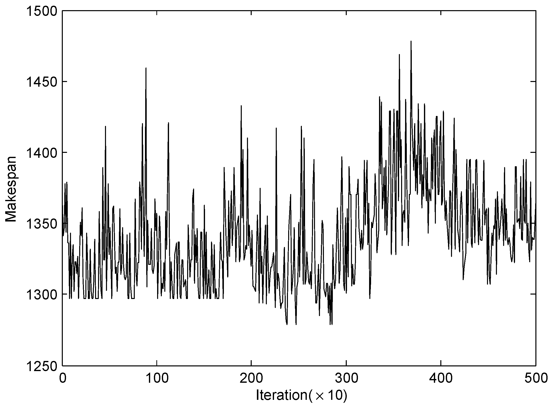
Before presenting the performance of the stochastic algorithm on the benchmark instances and comparing the results with the best available solutions in the literature, we present the internal operations and convergence of the algorithm in solving the instances ta001, and ta012. Figure 7 shows solution value versus iteration for 5000 iterations, for the instance ta001. As is seen, a high-quality solution can follow a low-quality one, and vice versa.

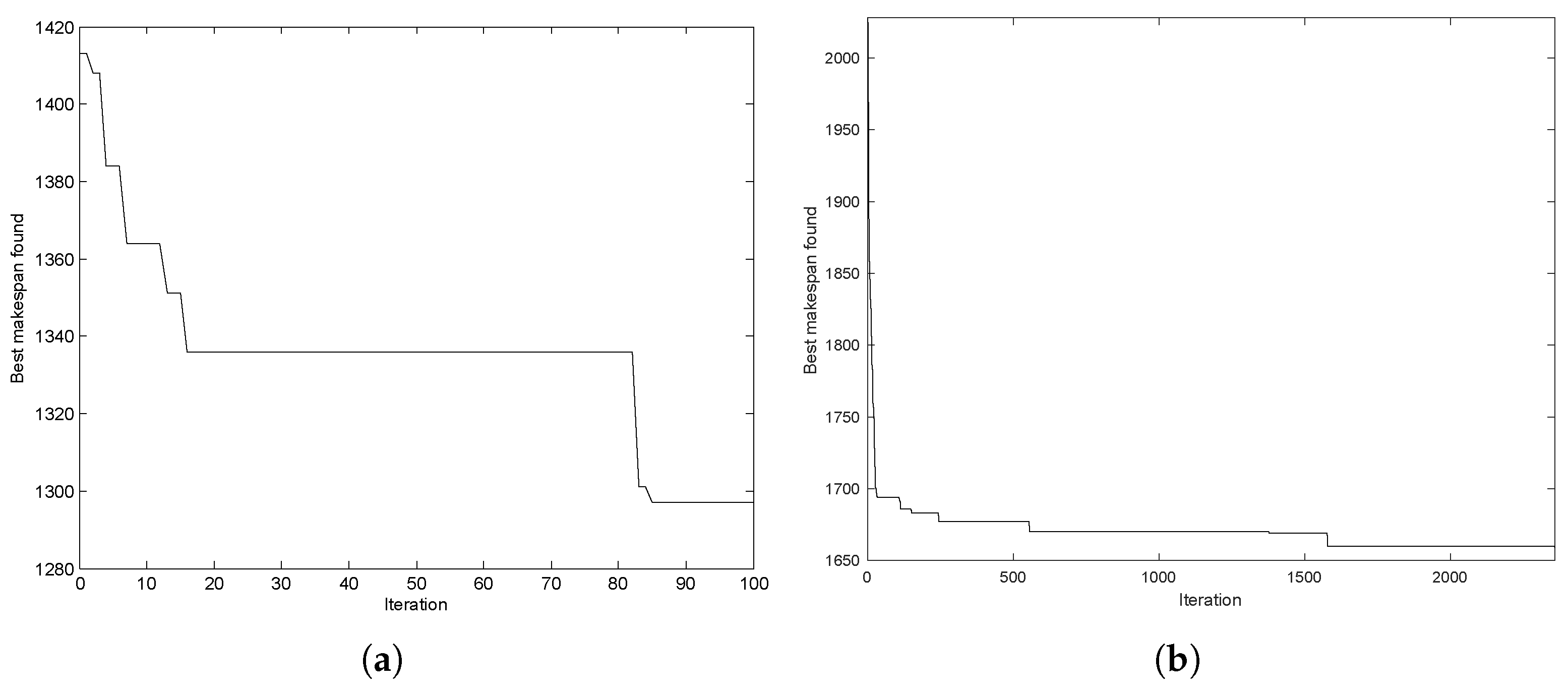
In general, the quality of the best solution obtained improves as the number of iterations increases. Figure 8a shows how this has happened in the first 100 iterations of the ta001 problem instance. As is seen, before iteration 20, the quality of the best-obtained solution has improved from 1413 to 1336 and for the next 60 iterations, no improvement has occurred. Between iterations 80 and 100, two other improvements have occurred and 1336 has improved to 1297. A similar trend can be seen in other instances as well; Figure 8b shows the convergence pattern, in just over 2000 iterations for a larger problem instance, ta012.

Comparison with Other Metaheuristics

RDIS is compared with a variety of metaheuristic in terms of solution quality and computation time. In particular, as presented in

Table 1. Comparison of average percent deviation with the best methods in the literature.

Group	Instances	Size	SAOP	ILS	M-MMAS	PACO	HGA_RMA	PSOVNS	NEGAVNS	RAMP	RDIS
1	ta001–ta010	20 × 5	1.05	0.33	0.04	0.18	0.04	0.03	0.00	0.00	0.00
2	ta011–ta020	20 × 10	2.60	0.52	0.07	0.24	0.02	0.02	0.01	0.03	0.03
3	ta021–ta030	20 × 20	2.06	0.28	0.06	0.18	0.05	0.05	0.02	0.04	0.04
4	ta031–ta040	50 × 5	0.34	0.18	0.02	0.05	0.00	0.00	0.00	0.00	0.01
5	ta041–ta050	50 × 10	3.50	1.45	1.08	0.81	0.72	0.57	0.82	0.37	0.95
6	ta051–ta060	50 × 20	4.66	2.05	1.93	1.41	0.99	1.36	1.08	0.61	1.88
7	ta061–ta070	100 × 5	0.30	0.16	0.02	0.02	0.01	0.00	0.00	0.00	0.01
8	ta071–ta080	100 × 10	1.34	0.64	0.39	0.29	0.16	0.18	0.14	0.06	0.38
9	ta081–ta090	100 × 20	4.49	2.42	2.42	1.93	1.30	1.45	1.40	1.76	2.35
10	ta091–ta100	200 × 10	0.94	0.50	0.30	0.23	0.14	0.18	0.16	0.15	0.32
11	ta101–ta110	200 × 20	3.67	2.07	2.15	1.82	1.26	1.35	1.25	2.00	2.30
12	ta111–ta120	500 × 20	2.20	1.20	1.02	0.85	0.69	–	0.71	1.20	1.32

, RDIS is compared with the Re-blocking Adjustable Memetic Procedure (RAMP) of [39] NEGA_VNS of [43], Particle swarm optimization algorithm, PSO_VNS, of [44], Simulated Annealing algorithm, SAOP, of [45], two Ant Colony Optimization algorithms, PACO and M-MMAS, due to [46], the iterated local search (ILS) of [47], and Hybrid genetic algorithm, HGA_RMA, of [48].

SAOP, PACO, M-MMAS, ILS and HGA_RMA are all run on a CPU with 2.6 GHz clock speed and the results are reported in [48]. However, RAMP and NEGA_VNS are run on a 2.2 GHz and a 2.4 GHz CPU respectively, and PSO_VNS is run on a 2.8 GHz CPU. Furthermore, CPU clock speeds are presented in

Table 2. Scaling factor computed for each CPU.

Algorithm	Clock Speed (GHz)	Scaling Factor
RDIS	2.2	1.00
RAMP	2.2	1.00
NEGAVNS	2.4	1.09
HGA_RMA	2.6	1.18
ILS	2.6	1.18
SAOP	2.6	1.18
M-MMAS	2.6	1.18
PACO	2.6	1.18
PSOVNS	2.8	1.27

and a scaling factor has been calculated. However, since CPU times depend on many factors such as developer skills, compiler efficiency, implementation details, and CPU architecture, any running time comparison should be made with caution.

Table 3. Comparison of maximum allowed running times for different metaheuristics.

			HGA_RMA		PSOVNS		NEGAVNS		RDIS / RAMP
Group	Instances	Size	Real	Scaled	Real	Scaled	Real	Scaled	Real	Scaled
1	ta001–ta010	20 × 5	4.5	5.31	300	381	10	10.9	10	10
2	ta011–ta020	20 × 10	9	10.62	300	381	20	21.8	20	20
3	ta021–ta030	20 × 20	18	21.24	300	381	40	43.6	40	40
4	ta031–ta040	50 × 5	11.3	13.334	300	381	25	27.25	25	25
5	ta041–ta050	50 × 10	22.5	26.55	300	381	50	54.5	50	50
6	ta051–ta060	50 × 20	45	53.1	300	381	100	109	100	100
7	ta061–ta070	100 × 5	22.5	26.55	600	762	50	54.5	50	50
8	ta071–ta080	100 × 10	45	53.1	600	762	100	109	100	100
9	ta081–ta090	100 × 20	90	106.2	600	762	200	218	200	200
10	ta091–ta100	200 × 10	90	106.2	600	762	200	218	200	200
11	ta101–ta110	200 × 20	180	212.4	600	762	400	436	400	400
12	ta111–ta120	500 × 20	450	531	–	–	1000	1090	1000	1000

shows the comparison of the real and scaled maximum allowed running time for RDIS, NEGA_VNS, PSO_VNS, and HGA_RMA. The maximum allowed running time of the other approaches in Table 3 is equal to that of HGA_RMA, since they are re-implemented and compared in [48]. Furthermore, since only NEGA_VNS and PSO_VNS have reported the average time needed to reach their best solution, a comparison is presented in

Table 4. Comparison of average time needed to reach the best solution for PSO_VNS, NEGA_VNS, RAMP, and RDIS.

			PSOVNS		NEGAVNS		RDIS / RAMP
Group	Instances	Size	Real	Scaled	Real	Scaled	Real	Scaled
1	ta001–ta010	20 × 5	13.5	17.145	2.2	2.4	0.0	0.0
2	ta011–ta020	20 × 10	26.3	33.401	12.2	13.3	0.3	0.3
3	ta021–ta030	20 × 20	69.3	88.011	29.2	31.8	13.5	13.5
4	ta031–ta040	50 × 5	2.8	3.556	8.2	8.9	0.1	0.1
5	ta041-ta050	50 × 10	79.8	101.346	32.3	35.2	19.9	19.9
6	ta051–ta060	50 × 20	168.1	213.487	55	60.0	34.3	34.3
7	ta061–ta070	100 × 5	52.6	66.802	30.8	33.6	1.5	1.5
8	ta071–ta080	100 × 10	211	267.97	58.7	64.0	39.3	39.3
9	ta081–ta090	100 × 20	310.8	394.716	122.7	133.7	75.0	75.0
10	ta091–ta100	200 × 10	191.3	242.951	134.5	146.6	49.8	49.8
11	ta101–ta110	200 × 20	438.7	557.149	271.7	296.2	170.0	170.0
12	ta111–ta120	500 × 20	–	–	523.4	570.5	482.3	482.3

.

In addition, based on the fact that NEGA_VNS, RAMP, and RDIS, allow similar maximum allowed running time (ref. Table 3), statistical testing has been performed to further analyze their difference. For this purpose, these methods are initially ranked based on their average deviation from the best-known solution %DEV_avg, for each instance group, as shown in

Table 5. NEGA_VNS, RAMP, and RDIS ranked based on %DEV_avg for each problem group.

Group	Instances	NEGAVNS	RAMP	RDIS
1	ta001–ta010	2.00	2.00	2.00
2	ta011–ta020	1.00	2.50	2.50
3	ta021–ta030	1.00	2.50	2.50
4	ta031–ta040	1.50	1.50	3.00
5	ta041–ta050	2.00	1.00	3.00
6	ta051–ta060	2.00	1.00	3.00
7	ta061–ta070	1.50	1.50	3.00
8	ta071–ta080	2.00	1.00	3.00
9	ta081–ta090	1.00	2.00	3.00
10	ta091–ta100	2.00	1.00	3.00
11	ta101–ta110	1.00	2.00	3.00
12	ta111–ta120	1.00	2.00	3.00

. In the case of tied %DEV_avg values, the average of the ranks with the assumption of no tied values, are calculated. The mean rank for NEGA_VNS, RAMP, and RDIS are 1.5, 1.667 and 2.833 respectively. Friedman test has been performed on the ranked data set, showing a statistically significant difference in the ranks, with ${\chi }^2\left(2\right)=15.2$, $p=0.0005$.

Further, for each pair of algorithms, post-hoc analysis using Wilcoxon signed-rank tests has been conducted with a significance level set at $p<(0.05/3=0.017)$ (Bonferroni correction). It has been found that there were no significant differences between the ranks of NEGA_VNS and RAMP (p = 0.482) but a significant difference between the ranks of NEGA_VNS, and RDIS (p < 0.001 ) as well as between RAMP and RDIS (p < 0.001). This could indicate that out of the three compared methods, NEGA_VNS and RAMP are the best performing ones and RDIS falls in second place. It is worth noting, these results should be interpreted with caution, as they are solely based on average deviation, and other factors such as best deviation, average and best running times, and implementation details have not been considered. An interested reader can see [49] for a tutorial on nonparametric statistical tests, used for comparing metaheuristics.

For a more fine-grained analysis, an instance-by-instance performance comparison is presented in

Table 6. Comparing the performance of the RDIS with that of NEGA_VNS for all individual instances.

						RDIS			NEGAVNS
Instance	n	m	LB	UB	NEH	Best	%DEVavg	Tbest	Best	%DEVavg	Tbest
ta001	20	5	1278	1278	1286	1278	0.00	0	1278	0.00	1
ta002	20	5	1359	1359	1365	1359	0.00	0	1359	0.00	2
ta003	20	5	1081	1081	1159	1081	0.00	0	1081	0.00	2
ta004	20	5	1293	1293	1325	1293	0.00	0	1293	0.00	2
ta005	20	5	1235	1235	1305	1235	0.00	0	1235	0.00	2
ta006	20	5	1195	1195	1228	1195	0.00	0	1195	0.00	3
ta007	20	5	1239	1239	1278	1239	0.00	0	1239	0.00	3
ta008	20	5	1206	1206	1223	1206	0.00	0	1206	0.00	2
ta009	20	5	1230	1230	1291	1230	0.00	0	1230	0.00	1
ta010	20	5	1108	1108	1151	1108	0.00	0	1108	0.00	4
ta011	20	10	1582	1582	1680	1582	0.00	0	1582	0.00	10
ta012	20	10	1659	1659	1729	1659	0.00	0	1659	0.02	9
ta013	20	10	1496	1496	1557	1496	0.02	2	1496	0.00	12
ta014	20	10	1377	1377	1439	1377	0.04	0	1377	0.05	17
ta015	20	10	1419	1419	1502	1419	0.00	0	1419	0.00	11
ta016	20	10	1397	1397	1453	1397	0.00	0	1397	0.00	15
ta017	20	10	1484	1484	1562	1484	0.00	0	1484	0.00	11
ta018	20	10	1538	1538	1609	1538	0.24	0	1538	0.00	10
ta019	20	10	1593	1593	1647	1593	0.00	0	1593	0.00	13
ta020	20	10	1591	1591	1653	1591	0.00	1	1591	0.00	14
ta021	20	20	2297	2297	2410	2297	0.05	14	2297	0.00	26
ta022	20	20	2099	2099	2150	2099	0.06	36	2099	0.01	33
ta023	20	20	2326	2326	2411	2326	0.09	24	2326	0.02	32
ta024	20	20	2223	2223	2262	2223	0.03	2	2223	0.00	22
ta025	20	20	2291	2291	2397	2291	0.10	34	2291	0.04	21
ta026	20	20	2226	2226	2349	2226	0.09	18	2226	0.03	35
ta027	20	20	2273	2273	2362	2273	0.00	2	2273	0.07	36
ta028	20	20	2200	2200	2249	2200	0.00	3	2200	0.00	25
ta029	20	20	2237	2237	2320	2237	0.00	0	2237	0.00	23
ta030	20	20	2178	2178	2277	2178	0.01	1	2178	0.02	39
ta031	50	5	2724	2724	2733	2724	0.00	0	2724	0.00	6
ta032	50	5	2834	2834	2843	2836	0.09	0	2834	0.00	5
ta033	50	5	2621	2621	2640	2621	0.00	0	2621	0.00	1
ta034	50	5	2751	2751	2782	2751	0.00	0	2751	0.00	11
ta035	50	5	2863	2863	2868	2863	0.01	1	2863	0.00	8
ta036	50	5	2829	2829	2850	2829	0.00	0	2829	0.00	5
ta037	50	5	2725	2725	2758	2725	0.00	0	2725	0.00	7
ta038	50	5	2683	2683	2721	2683	0.00	0	2683	0.00	6
ta039	50	5	2552	2552	2576	2552	0.00	0	2552	0.00	12
ta040	50	5	2782	2782	2790	2782	0.00	0	2782	0.00	21
ta041	50	10	2991	2991	3135	3025	1.34	21	3021	1.03	38
ta042	50	10	2867	2867	3032	2911	1.67	2	2902	1.28	41
ta043	50	10	2839	2839	2986	2871	1.25	5	2871	1.14	36
ta044	50	10	3063	3063	3198	3064	0.09	5	3070	0.28	29
ta045	50	10	2976	2976	3160	3005	1.18	23	2998	0.81	25
ta046	50	10	3006	3006	3178	3012	0.68	23	3024	0.68	32
ta047	50	10	3093	3093	3277	3126	1.23	43	3122	0.98	19
ta048	50	10	3037	3037	3123	3042	0.28	25	3063	0.93	29
ta049	50	10	2897	2897	3002	2905	0.43	8	2914	0.65	39
ta050	50	10	3065	3065	3257	3099	1.37	43	3076	0.44	35
ta051	50	20	3771	3850	4082	3917	1.92	73	3874	0.77	22
ta052	50	20	3668	3704	3921	3757	1.77	70	3734	1.02	87
ta053	50	20	3591	3640	3927	3699	2.26	11	3688	1.39	56
ta054	50	20	3635	3720	3969	3781	1.86	1	3759	1.14	39
ta055	50	20	3553	3610	3835	3673	2.08	8	3644	1.03	48
ta056	50	20	3667	3681	3914	3716	1.35	60	3717	1.07	74
ta057	50	20	3672	3704	3952	3769	1.83	39	3728	0.79	42
ta058	50	20	3627	3691	3938	3759	2.25	40	3730	1.18	28
ta059	50	20	3645	3743	3952	3790	1.76	5	3779	1.10	90
ta060	50	20	3696	3756	4079	3809	1.72	36	3801	1.35	64

and

Table 7. (continued) Comparing the performance of the RDIS with that of NEGA_VNS for all individual instances.

						RDIS			NEGAVNS
Instance	n	m	LB	UB	NEH	Best	%DEVavg	Tbest	Best	%DEVavg	Tbest
ta061	100	5	5493	5493	5519	5493	0.00	0	5493	0.00	34
ta062	100	5	5268	5268	5348	5268	0.04	13	5268	0.00	26
ta063	100	5	5175	5175	5219	5175	0.00	0	5175	0.00	36
ta064	100	5	5014	5014	5023	5014	0.03	1	5014	0.00	33
ta065	100	5	5250	5250	5266	5250	0.00	0	5250	0.00	12
ta066	100	5	5135	5135	5139	5135	0.00	0	5135	0.00	42
ta067	100	5	5246	5246	5259	5246	0.00	0	5246	0.00	50
ta068	100	5	5094	5094	5120	5094	0.00	0	5094	0.00	31
ta069	100	5	5448	5448	5489	5448	0.00	0	5448	0.00	25
ta070	100	5	5322	5322	5341	5322	0.03	1	5322	0.00	19
ta071	100	10	5770	5770	5846	5779	0.21	19	5770	0.04	49
ta072	100	10	5349	5349	5453	5353	0.22	99	5358	0.23	78
ta073	100	10	5676	5676	5824	5679	0.05	0	5676	0.09	65
ta074	100	10	5781	5781	5929	5808	0.63	65	5792	0.23	22
ta075	100	10	5467	5467	5679	5483	0.62	71	5467	0.06	81
ta076	100	10	5303	5303	5375	5308	0.09	1	5311	0.20	72
ta077	100	10	5595	5595	5704	5599	0.08	4	5605	0.22	54
ta078	100	10	5617	5617	5760	5646	0.71	72	5617	0.05	64
ta079	100	10	5871	5871	6032	5918	0.90	57	5877	0.19	29
ta080	100	10	5845	5845	5918	5850	0.30	5	5845	0.09	73
ta081	100	20	6106	6202	6541	6369	2.85	25	6303	1.69	85
ta082	100	20	6183	6183	6523	6303	2.09	14	6266	1.45	75
ta083	100	20	6252	6271	6639	6385	2.02	4	6351	1.32	145
ta084	100	20	6254	6269	6557	6364	1.79	63	6360	1.49	129
ta085	100	20	6262	6314	6695	6463	2.64	30	6408	1.57	163
ta086	100	20	6302	6364	6664	6487	2.17	16	6453	1.50	108
ta087	100	20	6184	6268	6632	6419	2.57	174	6332	1.10	94
ta088	100	20	6315	6401	6739	6551	2.81	201	6482	1.49	112
ta089	100	20	6204	6275	6677	6402	2.35	83	6343	1.15	169
ta090	100	20	6404	6434	6677	6562	2.22	141	6506	1.26	147
ta091	200	10	10,862	10,862	10,942	10,885	0.25	30	10,885	0.24	89
ta092	200	10	10,480	10,480	10,716	10,503	0.45	76	10,495	0.19	125
ta093	200	10	10,922	10,922	11,025	10,965	0.49	135	10,941	0.21	169
ta094	200	10	10,889	10,889	11,057	10,893	0.09	27	10,889	0.04	158
ta095	200	10	10,524	10,524	10,645	10,528	0.11	30	10,524	0.03	192
ta096	200	10	10,329	10,329	10,458	10,337	0.16	31	10,346	0.21	91
ta097	200	10	10,854	10,854	10,989	10,883	0.43	22	10,866	0.17	124
ta098	200	10	10,730	10,730	10,829	10,769	0.44	12	10,741	0.15	112
ta099	200	10	10,438	10,438	10,574	10,465	0.26	9	10,451	0.19	138
ta100	200	10	10,675	10,675	10,807	10,722	0.48	125	10,684	0.14	147
ta101	200	20	11,152	11,195	11,594	11,399	2.05	224	11,339	1.52	222
ta102	200	20	11,143	11,203	11,675	11,482	2.73	302	11,344	1.47	268
ta103	200	20	11,281	11,281	11,852	11,535	2.52	165	11,445	1.45	385
ta104	200	20	11,275	11,275	11,803	11,501	2.27	118	11,434	1.49	154
ta105	200	20	11,259	11,259	11,685	11,449	1.81	130	11,369	1.06	300
ta106	200	20	11,176	11,176	11,629	11,413	2.40	148	11,292	1.01	254
ta107	200	20	11,337	11,360	11,833	11,555	2.09	114	11,481	1.11	269
ta108	200	20	11,301	11,334	11,913	11,554	2.12	49	11,442	1.03	311
ta109	200	20	11,145	11,192	11,673	11,473	2.64	342	11,313	1.22	326
ta110	200	20	11,284	11,288	11,869	11,517	2.34	109	11,424	1.14	228
ta111	500	20	26,040	26,059	26,670	26,448	1.60	344	26,228	0.73	311
ta112	500	20	26,500	26,520	27,232	26,938	1.70	453	26,688	0.77	552
ta113	500	20	26,371	26,371	26,848	26,730	1.47	348	26,522	0.71	448
ta114	500	20	26,456	26,456	27,055	26,721	1.16	600	26,586	0.54	269
ta115	500	20	26,334	26,334	26,727	26,606	1.14	220	26,541	0.82	396
ta116	500	20	26,469	26,477	26,992	26,729	1.14	284	26,582	0.49	682
ta117	500	20	26,389	26,389	26,797	26,643	1.10	759	26,660	1.12	559
ta118	500	20	26,560	26,560	27,138	26,858	1.32	970	26,711	0.61	814
ta119	500	20	26,005	26,005	26,631	26,348	1.49	36	26,148	0.61	592
ta120	500	20	26,457	26,457	26,984	26,698	1.08	808	26,611	0.67	611

. In these tables, the performance of the RDIS on these instances is shown and compared with that of the NEGA_VNS presented in [43]. The NEGA_VNS, which is a genetic algorithm (GA) and uses the variable neighborhood search (VNS) employs the NEH heuristic presented in [26] for constructing its initial solutions, and that is why it has been named as NEGA_VNS. The NEH has also been named as the initial of its authors and is a famous algorithm. As further information, the performance of the NEH has also been provided in the table.

In line with [43] (Zobolas, Tarantilis et al. 2009), we have set the running time of the RDIS to $(n\ast m)/10$ seconds for each run. Moreover, for removing the effect of the random seed and in line with other algorithms, the RDIS has been run 10 times for each instance, with different random seeds.

In Table 6 and Table 7, columns 2 and 3 represent the number of jobs and machines, respectively, and columns 4 and 5 show the lower and upper bound of each instance. The value of the upper bound is the best available makespan for the corresponding instance in the literature, and in the cases where upper and lower bounds are equal, the best available makespan in the literature is equal to the optimal solution.

Columns 6, 7, and 10 provide the values of the makespan produced by NEH, RDIS, and NEGA_VNS, respectively. The value of T_best shows the shortest time taken for the best solution to be obtained in seconds, and the value of %DEV_avg shows the average of the percentage deviation from the best available makespan. The percentage deviation from the best available makespan has been calculated based on the formula of $(s-UB)/UB$, in which s and $UB$ show the corresponding makespan calculated and the best available makespan, which is also an upper bound for the corresponding instance. The wide spectrum information provided in Table 6 and Table 7, based on 120 benchmark instances, indicates that the RDIS is highly competitive and produces comparatively high-quality solutions.

In all 120 instances, the RDIS has obtained a better solution value than the NEH heuristic. In terms of best solution value, the RDIS has obtained equal or better value in 61 out of 120 problems. Moreover, in 46 out of 120 instances the average percentage deviation has been smaller than or equal to that of the NEGA_VNS, and in 100 out of 120 instances, the average shortest time to find the best solution is less than or equal to that of the NEGA_VNS. Moreover, the total average running times to reach the best solution of RDIS is more than 44 times faster than that of NEGA_VNS.

6. Concluding Remarks

In the area of algorithm design, the notion of decomposition is an umbrella term for obtaining a solution to a problem through its break-down into subproblems, with all these subproblems being handled with the same procedure. The RDIS is a stochastic algorithm based on such notion, in the sense that it translates non-tractable problems to tractable subproblems and obtains optimal solutions of these tractable subproblems.

The integration of the optimal sub-solutions provided for these subproblems, expectedly does not lead to the overall optimal solution, except for small-sized problems. However, computational experiments have shown that the RDIS is able to produce solutions with the accuracy of one percent from the best-known solutions in the literature. This success is not the result of one factor but that of three major factors.

First, the combination of small and large neighborhood schemes is able to create a delicate balance between speed and quality. With this respect, it should be noticed that although in local searches multi-exchanges usually lead to better results than that of pair-exchanges, nevertheless, multi-exchanges require outsized execution times.

In other words, in the RDIS, the size of k-exchange neighborhood is not $O\left(\left(\genfrac{}{}{0pt}{}{n}{k}\right)\right)$, as it is the case with other k-exchange neighborhoods, but only a tiny fraction of it. The reason is that in the RDIS, the computational burden has been placed on the small neighborhood scheme and the large neighborhood scheme is used only for promising partitions, taking an immense bulk of possible k-exchanges out of considerations and contributing to the efficiency of the stochastic algorithm.

Second, the RJP, as a construction method, is able to successively rearrange jobs through informed revisions, and this makes the quality of initial solutions for the local searches high. To further emphasize the role of such informed decisions in increasing solution quality, we can mention similar algorithms like the ant colony optimization, which have simply built upon construction methods but can even compete with local searches.

Third, varying the initial permutation through randomly swapping the neighboring jobs, with the chance of SwapProb, not only has diversified the search but it has led to the feature of not losing the accumulated knowledge regarding the best permutation of jobs initially obtained by the RJP. With respect to this feature, the issue is not simply that the random swapping of jobs diversifies the permutation initially obtained by the RJP and allows different starting points to be generated. The deeper issue is that since the RJP does not care about the position of two neighboring jobs and mainly concentrates on grouping the jobs in two partitions, these random swaps, despite their contribution to diversification, cannot significantly degrade the quality of the original permutation proposed by the RJP.

The RDIS can be improved in several directions as outlined in the following:

• Trivial as well as sophisticated implementation of parallelization techniques;
• Efficient estimation, instead of exact evaluation, of the makespan; and
• Integration with population-based techniques.

For enhancing the algorithm through the concept of parallelization, it is possible to employ this concept in a range from its trivial implementation to its most sophisticated structure. In its trivial implementation, several threads of the same procedure can start on a number of processors with different initial solutions.

In its sophisticated structure, however, parallelization can be employed for the entire algorithm as an integrated entity. In this case, two groups of threads need to be developed. In the first group, each thread can calculate the makespan of one neighbor on a separate processor, regardless of whether a small or large neighborhood is in place.

On the other hand, in the second group, each thread can be assigned to solving a two-machine problem. Since nearly the entire time of local searches is spent on calculating the values of makespan and the entire time of the RJP is spent on solving the two-machine problems, this form of parallelization speeds up the algorithm and enables the enhanced procedure to tackle larger instances more efficiently.

The other promising direction for further enhancing the RDIS is the development of novel evaluation functions. Considering the fact that a large percentage of computation time in a typical local search is spent on calculating the exact values of the makespan, the development of novel evaluation functions, which with significant precision can efficiently estimate such values, can decrease the search effort and work towards search efficiency. Based on such ease of calculation, which is obtained at the loss of insignificant precision, the local search can probe larger parts of the search space and, if conducted properly, can obtain high-quality solutions.

The final suggestion for enhancing the RDIS is the development of a population-based mechanism that can work with the current point-based local searches employed. Such a mechanism can govern how computation time is devoted to manipulating solutions with higher quality, and in this way, it can prevent solutions with lower quality from seizing computational resources. The proposed population-based mechanism can also spread the characteristics of high-quality solutions in other individuals of the population. Since, as the population is evolved, the genetic diversity among the individuals of the population declines and the population becomes homogeneous, the design of proper mutation operators exploiting the structure of the PFSP is of key importance in implementing such a possible population-based mechanism.

References

- Ahuja, R.; Jha, K.; Orlin, J.; Sharma, D. Very large-scale neighborhood search for the quadratic assignment problem. INFORMS J. Comput. 2007, 19, 646–657. [Google Scholar] [CrossRef] [Green Version]
- Hansen, P.; Mladenović, N. Variable Neighborhood Search. In Handbook of Metaheuristics; Glover, F., Kochenberger, G.A., Eds.; Springer: Boston, MA, USA, 2003; pp. 145–184. [Google Scholar] [CrossRef] [Green Version]
- Ahuja, R.K.; Ergun, Ö.; Orlin, J.B.; Punnen, A.P. A survey of very large-scale neighborhood search techniques. Discret. Appl. Math. 2002, 123, 75–102. [Google Scholar] [CrossRef] [Green Version]
- Johnson, S. Optimal two and three machine production scheduling with set up times included. Nav. Res. Logist. 1954, 1, 61–68. [Google Scholar] [CrossRef]
- Garey, M.; Johnson, D.; Sethi, R. The complexity of flowshop and jobshop scheduling. Math. Oper. Res. 1976, 1, 117–129. [Google Scholar] [CrossRef]
- Jackson, J. An extension of Johnson’s results on job IDT scheduling. Nav. Res. Logist. Q. 1956, 3, 201–203. [Google Scholar] [CrossRef]
- Burns, F.; Rooker, J. Technical Note—Three-Stage Flow-Shops with Recessive Second Stage. Oper. Res. 1978, 26, 207–208. [Google Scholar] [CrossRef] [Green Version]
- Baioletti, M.; Milani, A.; Santucci, V. MOEA/DEP: An Algebraic Decomposition-Based Evolutionary Algorithm for the Multiobjective Permutation Flowshop Scheduling Problem. In Evolutionary Computation in Combinatorial Optimization; Liefooghe, A., López-Ibáñez, M., Eds.; Springer International Publishing: Cham, Switzerland, 2018; pp. 132–145. [Google Scholar]
- Shao, Z.; Shao, W.; Pi, D. Effective heuristics and metaheuristics for the distributed fuzzy blocking flow-shop scheduling problem. Swarm Evol. Comput. 2020, 59, 100747. [Google Scholar] [CrossRef]
- Caldeira, R.H.; Gnanavelbabu, A.; Vaidyanathan, T. An effective backtracking search algorithm for multi-objective flexible job shop scheduling considering new job arrivals and energy consumption. Comput. Ind. Eng. 2020, 149, 106863. [Google Scholar] [CrossRef]
- Rinnoy Kan, A. Machine Scheduling Problems: Classification, Complexity and Computation; Martinus Nijhoff Hague: Leiden, Belgium, 1976. [Google Scholar]
- Röck, H. The three-machine no-wait flow shop is NP-complete. JACM 1984, 31, 336–345. [Google Scholar] [CrossRef]
- Naderi, B.; Ruiz, R. The distributed permutation flowshop scheduling problem. Comput. Oper. Res. 2010, 37, 754–768. [Google Scholar] [CrossRef]
- Wang, G.; Gao, L.; Li, X.; Li, P.; Tasgetiren, M.F. Energy-efficient distributed permutation flow shop scheduling problem using a multi-objective whale swarm algorithm. Swarm Evol. Comput. 2020, 57, 100716. [Google Scholar] [CrossRef]
- Dudek, R.; Panwalkar, S.; Smith, M. The lessons of flowshop scheduling research. Oper. Res. 1992, 40, 7–13. [Google Scholar] [CrossRef] [Green Version]
- Blazewicz, J.; Domschke, W.; Pesch, E. The job shop scheduling problem: Conventional and new solution techniques. Eur. J. Oper. Res. 1996, 93, 1–33. [Google Scholar] [CrossRef]
- Framinan, J.M.; Gupta, J.N.D.; Leisten, R. A review and classification of heuristics for permutation flow-shop scheduling with makespan objective. J. Oper. Res. Soc. 2004, 55, 1243–1255. [Google Scholar] [CrossRef]
- Palmer, D. Sequencing jobs through a multi-stage process in the minimum total time—A quick method of obtaining a near optimum. J. Oper. Res. Soc. 1965, 16, 101–107. [Google Scholar] [CrossRef]
- Bonney, M.; Gundry, S. Solutions to the constrained flowshop sequencing problem. Oper. Res. Q. 1976, 27, 869–883. [Google Scholar] [CrossRef]
- Pajak, Z. The slope-index technique for scheduling in machine shop. In Current Production Scheduling Practice Conference; Tate, T., Ed.; University of London: London, UK, 1971. [Google Scholar]
- Gupta, J.N. A general algorithm for m*n flowshop scheduling problem. Int. J. Prod. Res. 1969, 7, 241. [Google Scholar] [CrossRef]
- Campbell, H.; Dudek, R.; Smith, M. A heuristic algorithm for the n job, m machine sequencing problem. Manag. Sci. 1970, 16, 630–637. [Google Scholar] [CrossRef] [Green Version]
- Turner, S.; Booth, D. Comparison of heuristics for flow shop sequencing. Omega 1987, 15, 75–78. [Google Scholar] [CrossRef]
- Widmer, M.; Hertz, A. A new heuristic method for the flow shop sequencing problem. Eur. J. Oper. Res. 1989, 41, 186–193. [Google Scholar] [CrossRef]
- Moccellin, J.V. A New Heuristic Method for the Permutation Flow Shop Scheduling Problem. J. Oper. Res. Soc. 1995, 46, 883–886. [Google Scholar] [CrossRef]
- Nawaz, M.; Enscore, E.; Ham, I. A heuristic algorithm for the m-machine n-job flow-shop sequencing problem. Omega 1983, 11, 91–95. [Google Scholar] [CrossRef]
- Liu, W.; Jin, Y.; Price, M. A new improved NEH heuristic for permutation flowshop scheduling problems. Int. J. Prod. Econ. 2017, 193, 21–30. [Google Scholar] [CrossRef] [Green Version]
- Ruiz, R.; Stützle, T. A simple and effective iterated greedy algorithm for the permutation flowshop scheduling problem. Eur. J. Oper. Res. 2007, 177, 2033–2049. [Google Scholar] [CrossRef]
- Ogbu, F.; Smith, D. The application of the simulated annealing algorithm to the solution of the n/m/Cmax flowshop problem. Comput. Oper. Res. 1990, 17, 243–253. [Google Scholar] [CrossRef]
- Taillard, E. Some efficient heuristic methods for the flow shop sequencing problem. Eur. J. Oper. Res. 1990, 47, 65–74. [Google Scholar] [CrossRef]
- Nowicki, E.; Smutnicki, C. A fast tabu search algorithm for the permutation flow-shop problem. Eur. J. Oper. Res. 1996, 91, 160–175. [Google Scholar] [CrossRef]
- Reeves, C. A genetic algorithm for flowshop sequencing. Comput. Oper. Res. 1995, 22, 5–13. [Google Scholar] [CrossRef]
- Nowicki, E.; Smutnicki, C. Some aspects of scatter search in the flow-shop problem. Eur. J. Oper. Res. 2006, 169, 654–666. [Google Scholar] [CrossRef]
- Iyer, S.; Saxena, B. Improved genetic algorithm for the permutation flowshop scheduling problem. Comput. Oper. Res. 2004, 31, 593–606. [Google Scholar] [CrossRef]
- Yagmahan, B.; Yenisey, M. A multi-objective ant colony system algorithm for flow shop scheduling problem. Expert Syst. Appl. 2010, 37, 1361–1368. [Google Scholar] [CrossRef]
- Lian, Z.; Gu, X.; Jiao, B. A novel particle swarm optimization algorithm for permutation flow-shop scheduling to minimize makespan. Chaos Solitons Fractals 2008, 35, 851–861. [Google Scholar] [CrossRef]
- Liu, Y.F.; Liu, S.Y. A hybrid discrete artificial bee colony algorithm for permutation flowshop scheduling problem. Appl. Soft Comput. 2013, 13, 1459–1463. [Google Scholar] [CrossRef]
- Santucci, V.; Baioletti, M.; Milani, A. Solving permutation flowshop scheduling problems with a discrete differential evolution algorithm. AI Commun. 2016, 29, 269–286. [Google Scholar] [CrossRef]
- Amirghasemi, M.; Zamani, R. An Effective Evolutionary Hybrid for Solving the Permutation Flowshop Scheduling Problem. Evol. Comput. 2017, 25, 87–111. [Google Scholar] [CrossRef]
- Fernandez-Viagas, V.; Ruiz, R.; Framinan, J.M. A new vision of approximate methods for the permutation flowshop to minimise makespan: State-of-the-art and computational evaluation. Eur. J. Oper. Res. 2017, 257, 707–721. [Google Scholar] [CrossRef]
- Nowicki, E.; Smutnicki, C. A fast taboo search algorithm for the job shop problem. Manag. Sci. 1996, 42, 797–813. [Google Scholar] [CrossRef]
- Taillard, E. Benchmarks for basic scheduling problems. Eur. J. Oper. Res. 1993, 64, 278–285. [Google Scholar] [CrossRef]
- Zobolas, G.; Tarantilis, C.D.; Ioannou, G. Minimizing makespan in permutation flow shop scheduling problems using a hybrid metaheuristic algorithm. Comput. Oper. Res. 2009, 36, 1249–1267. [Google Scholar] [CrossRef]
- Tasgetiren, M.F.; Liang, Y.C.; Sevkli, M.; Gencyilmaz, G. A particle swarm optimization algorithm for makespan and total flowtime minimization in the permutation flowshop sequencing problem. Eur. J. Oper. Res. 2007, 177, 1930–1947. [Google Scholar] [CrossRef]
- Osman, I.H.; Potts, C.N. Simulated annealing for permutation flow-shop scheduling. Omega 1989, 17, 551–557. [Google Scholar] [CrossRef]
- Rajendran, C.; Ziegler, H. Ant-colony algorithms for permutation flowshop scheduling to minimize makespan/total flowtime of jobs. Eur. J. Oper. Res. 2004, 155, 426–438. [Google Scholar] [CrossRef]
- Stützle, T. Applying Iterated Local Search to the Permutation Flow Shop Problem; Technical Report, Technical Report AIDA-98-04; FG Intellektik, TU Darmstadt: Darmstadt, Germany, 1998. [Google Scholar]
- Ruiz, R.; Maroto, C.; Alcaraz, J. Two new robust genetic algorithms for the flowshop scheduling problem. Omega 2006, 34, 461–476. [Google Scholar] [CrossRef]
- Derrac, J.; García, S.; Molina, D.; Herrera, F. A practical tutorial on the use of nonparametric statistical tests as a methodology for comparing evolutionary and swarm intelligence algorithms. Swarm Evol. Comput. 2011, 1, 3–18. [Google Scholar] [CrossRef]
Figure 1.
A sample 4-job 4-machine Permutation Flow-shop Scheduling Problem (PFSP) problem, with the permutation of (1,2,3,4) of jobs leading to the solution value of 30.
Figure 2.
Changing the order of (1,2,3,4) to (1,4,3,2) in the sample problem and obtaining the optimal solution with the makespan of 29.
Figure 3.
The c-type pseudocode of the Refining Decomposition-based Integrated Search (RDIS) algorithm.
Figure 4.
The flowchart of the the main steps of the RDIS algorithm.
Figure 5.
The c-type pseudocode of largeNeighbourhoodSearch.
Figure 6.
Changing the order of (1,2,3,4,5,6,7,8) to (3,1,2,6,4,8,7,5) in a sample 8 8 problem in 3 steps, with each step optimizing a chunk of size 4.
Figure 7.
Solution value versus iteration in the benchmark instance ta001.
Figure 8.
So-far-Best solution versus iteration in the benchmark instances ta001 (a) and ta012 (b).