
On a Robust and Efficient Numerical Scheme for the Simulation of Stationary 3-Component Systems with Non-Negative Species-Concentration with an Application to the Cu Deposition from a Cu-(β-alanine)-Electrolyte


Abstract
:1. Introduction
2. A Generalized Mathematical Model
2.1. The Classical Approach
2.2. Reinforcing Non-Negative Species Distributions
3. Numerical Scheme
| Algorithm 1: augmented Lagrangian algorithm |
| Input: , , , , , , . Output: Approximate solution to (4) and approximation of the Lagrangian multiplier. Follow the steps
|
| Algorithm 2: Homotopie-Loop |
| Input: Inital discretization of the interval , system parameters , , , , and set , set initial value , . Output: Approximate solution to (8) and set . The homotopy algorithm is given through the following steps.
|
| Algorithm 3: AFEM-loop |
| Input: Initial regular triangulation , system parameters, set . Output: Fine mesh , approximate limit of the solutions to (13), estimation of the error. The adaptive FEM algorithm is given by the following steps:
|
- (i)
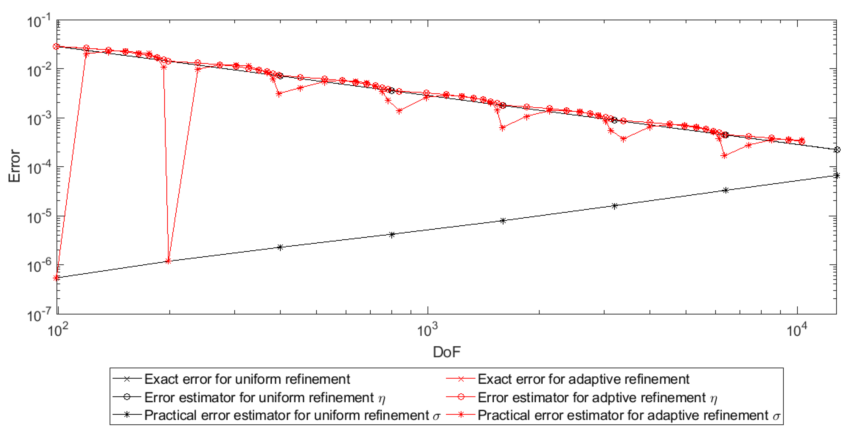
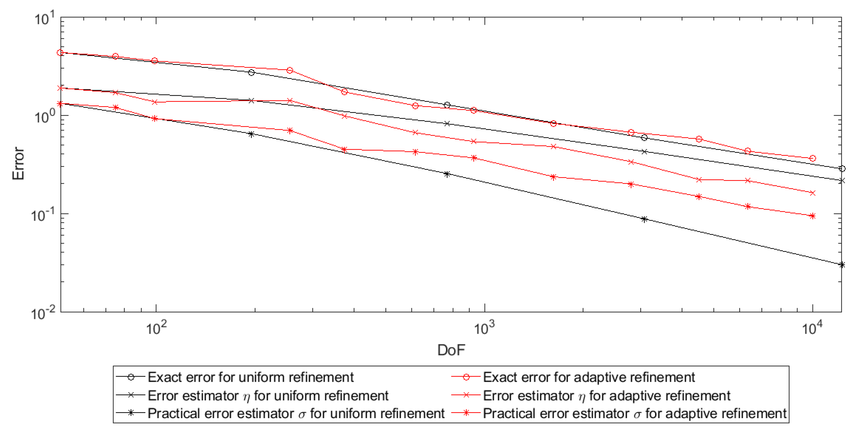
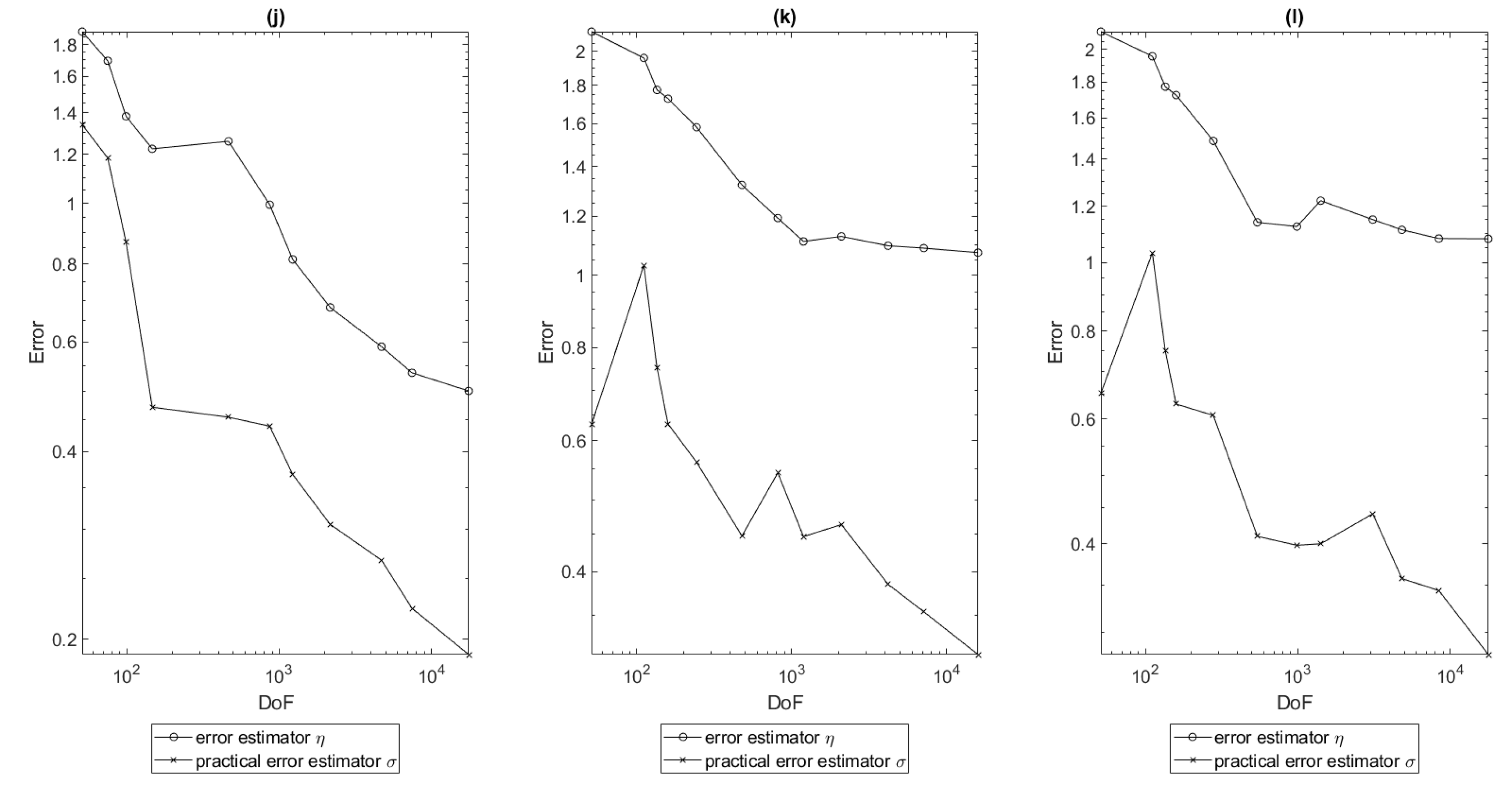
- In S2 of Algorithm 3, an estimator is evaluated on each element , which has to be defined. Assuming that for the exact solution of (3), the equalityholds true. In this paper, the estimator and the discrete solution of the discrete solution from S1: of Algorithm 3, for and , is defined as
- (ii)
- to hold true, since a solution of (5) is in general not a solution to a system of non-linear equations. Hence, the usage offor the solution of the discrete problem of S 1 of Algorithm 3, is not practical. In the spirit of the usage of adaptive schems an estimator τ, basing on ρ, is used, which gives an estimation on the local changes w.r.t. the elements of the evaluation of ρ. For the definition of a practical estimator let for an arbitrary fixed the element patch be given throughAfterwards, the new estimator σ is given through:
- (iii)
- A common strategy, used for the marking is the so-called Dörfler marking, cf. [49]. In this strategy, a set is chosen for which, , for a given bulk parameter the inequalityholds true.
- (iv)
- Note that the Dörfler marking implies for a simple uniform marking scheme.
- (v)
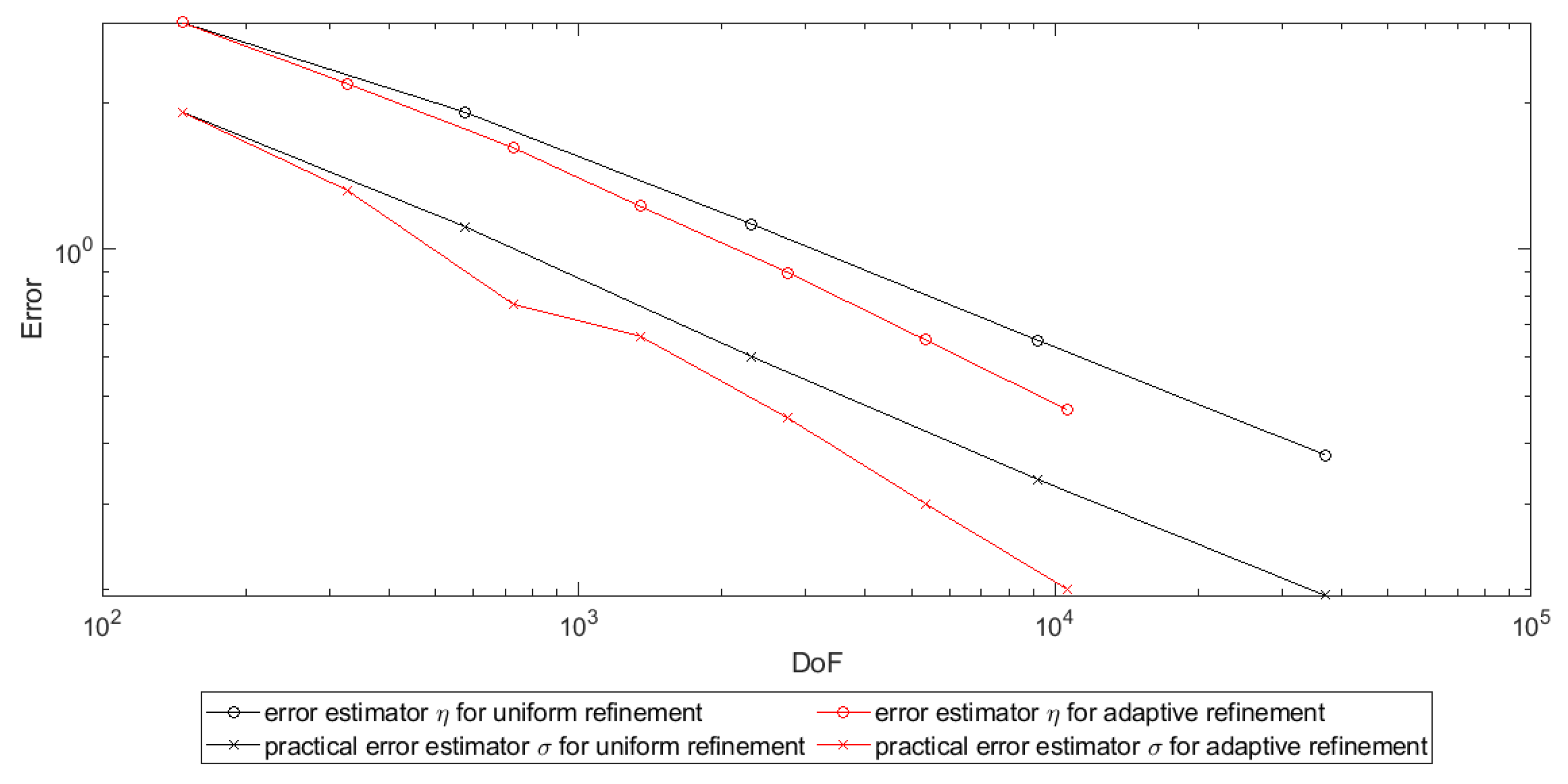
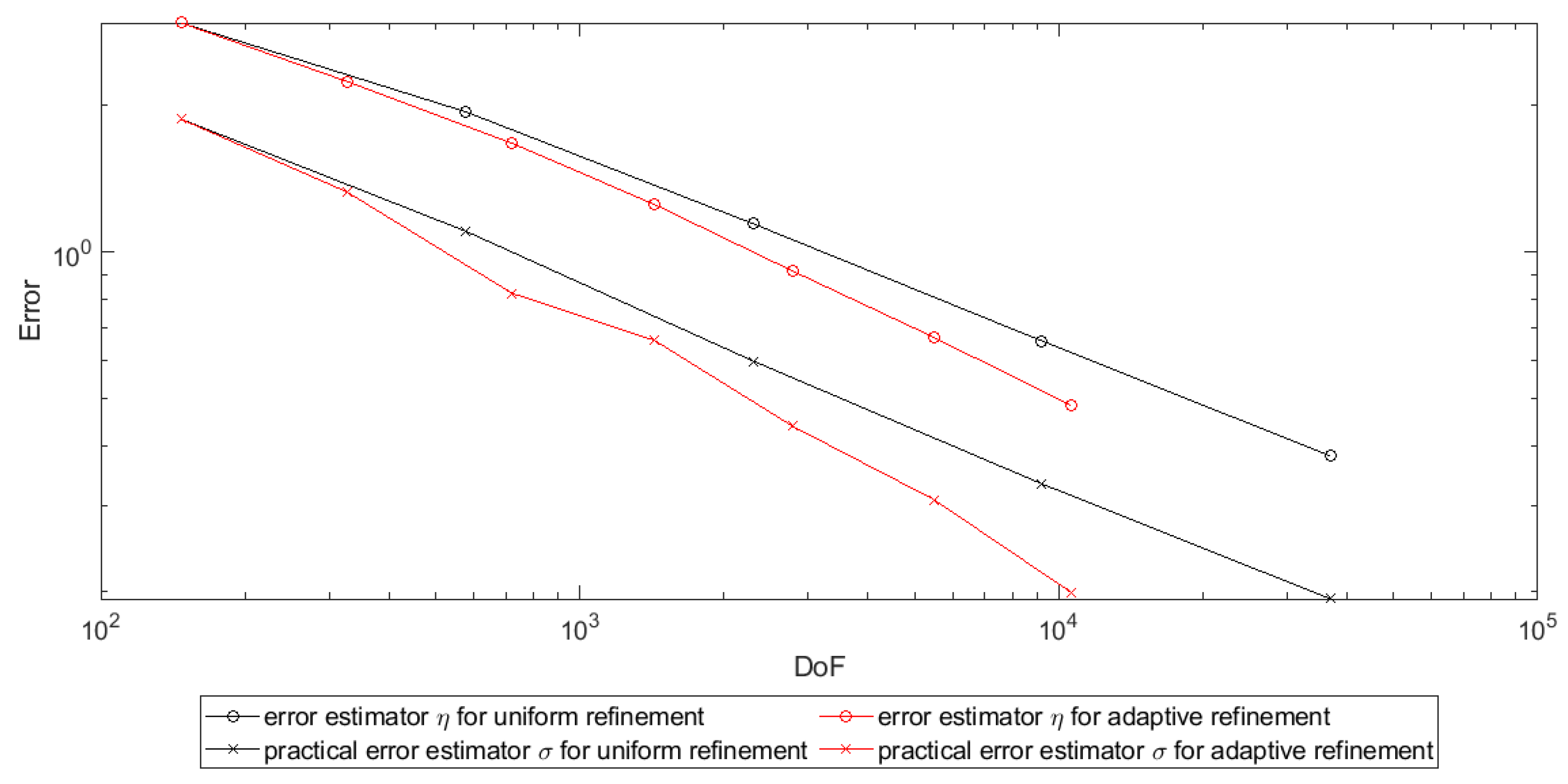
- As discussed in [50,51], one can usually prove convergence of the adaptive scheme by using, as in this article, the least-squares functional as error estimator, but cannot expect optimal convergence rates as discussed in [24] or [47]. Hence, another error estimator has to be derived for which optimal convergence rates are provable.
3.1. Remarks on Existence and Convergence Theory to the Numerical Scheme
3.1.1. Notes on the Existence Theory
- (i)
- (ii)
- (i)
- First, similar as in [52], the case of minimal assumptions to the problem formulation will be discussed. Essentially one assumes and the injectivity of the linear operator , used in the operator Equation (2a)–(2e). For this, one assumes that and are assumed to be chosen in a way that 0 is no eigenvalue of .Indeed, the injectivity, i.e., there is no 0-Eigenvalue of the corresponding operator, assumption together with the assumption of the existence of solutions for given , gives the unique solvability due to Fredholm’s alternative, cf. [53].The results above directly apply to the PDE equation that is given by
- (ii)
- Note that in (i) only necessary conditions for the unique solvability are discussed. Some sufficient conditions can be obtained by the decoupling of the PDE. Where in fact the sufficient conditions for the unique solvability can be obtained by sufficient conditions to scalar Diffusion reaction equations, cf. [33,54].
- (iii)
- By some standard calculations, as given in e.g., [19,28], one obtains that solves (3) if the first order optimality in form of the Euler–Lagrange equations is fulfilled, which is given by the following equation:Find such that for all the following equation holds true:
- (iv)
- (v)
- From the ellipticity of the bilinear form a, cf. (iv), one directly obtains the unique solvability of (4).
3.1.2. Notes on the Convergence Theory
- A similar interpretation, as in Remark 2 of the sequences and the inequality (21), indicate that there exists a constant , such that for initial values sufficiently close to the solution of (8) and the initial value are sufficiently close to the limit of the quasi-Newtonian scheme, the following inequality holds true:
- It directly follows
- (ii)
- The discussion (i) indicates that the quasi-Newtonian scheme described by the iterative solution by (13) has the same issue with stability as classical quasi-Newtonian schemes, cf. [17]. To stabilize the quasi-Newtonian scheme, it was coupled to a homotopy method, cf. [32]. As already discussed, the idea of the method is to solve for a continuous function , with and and a decomposition to solve the minimization problem that is given by:Find susch thatAs a solution step, the quasi-Newtonian scheme (13) can be used. For , an initial value for the algorithm is given through and for the is given as an initial value for the quasi-Newtonian scheme.
- (i)
- For every sequence , with , the following inequality holds true:
- (ii)
- For every , there exists a sequence with , such that the following inequality holds true:
- (i)
- ad (24): for the proof of this claim one needs to distinguish two cases. However, first, let and with be arbitrary fixed.
- (a)
- First, assume that up to finitely many one has . From the definition of it follows then that, up to finitely many , the lowest accumulation point of the sequence . Hence, one obtains the following inequality:The inequality above shows the assertion for this case.
- (b)
- For the second case, assume that there are infinitely many , such that . Subsequently, there exists a subsequence withBecause of the continuity of F and the definition of , it follows:The equalities above yield that the claim for the second case holds true.
The discussion of the two cases above proves the claim. - (ii)
- ad (25): first, note that, for all , one has a continuous embedding and is a dense subset of , c.f. [19,27,28,29]. Similarly, one has a continuous embedding furthermore is a dense subset of , c.f. [19,27,28,29]. From the definitions of and X, it follows with the both densities, where is a dense subset of X. From the assumptions on the sequence and the density of it follows that there exist, for all , a sequence with s.t. . Furthermore, it follows from the continuity of F and the definitions above:The equalities above prove the statement.From (i) and (ii), the claim of the Lemma follows by definition. □
- (i)
- (ii)
- (i)
- A common result in the context of -convergence, c.f. in [36,37,38,39], is that if -converges to then every accumulation point of the sequence of minimizers , i.e., minimizes , is a minimizer of G.Applying this theoretical result to the setup of Lemma 1, one obtains the statement in the corollary.
- (ii)
- The statement of the lemma directly follows by (i) and by (22).
- The convergence of the quasi-Newtonian scheme (13) has to be discussed in a much more rigorous way than done in Remark 5.
- Convergence to a certain rate has to be verified for the discretization of (5).
- As known to the authors, the existence theory, as described in Section 3.1.1, is for the problem (2a)–(2e) incomplete. A careful study of sufficient and necessary condition has to be made.
4. Numerical Examples and Validation of the Software
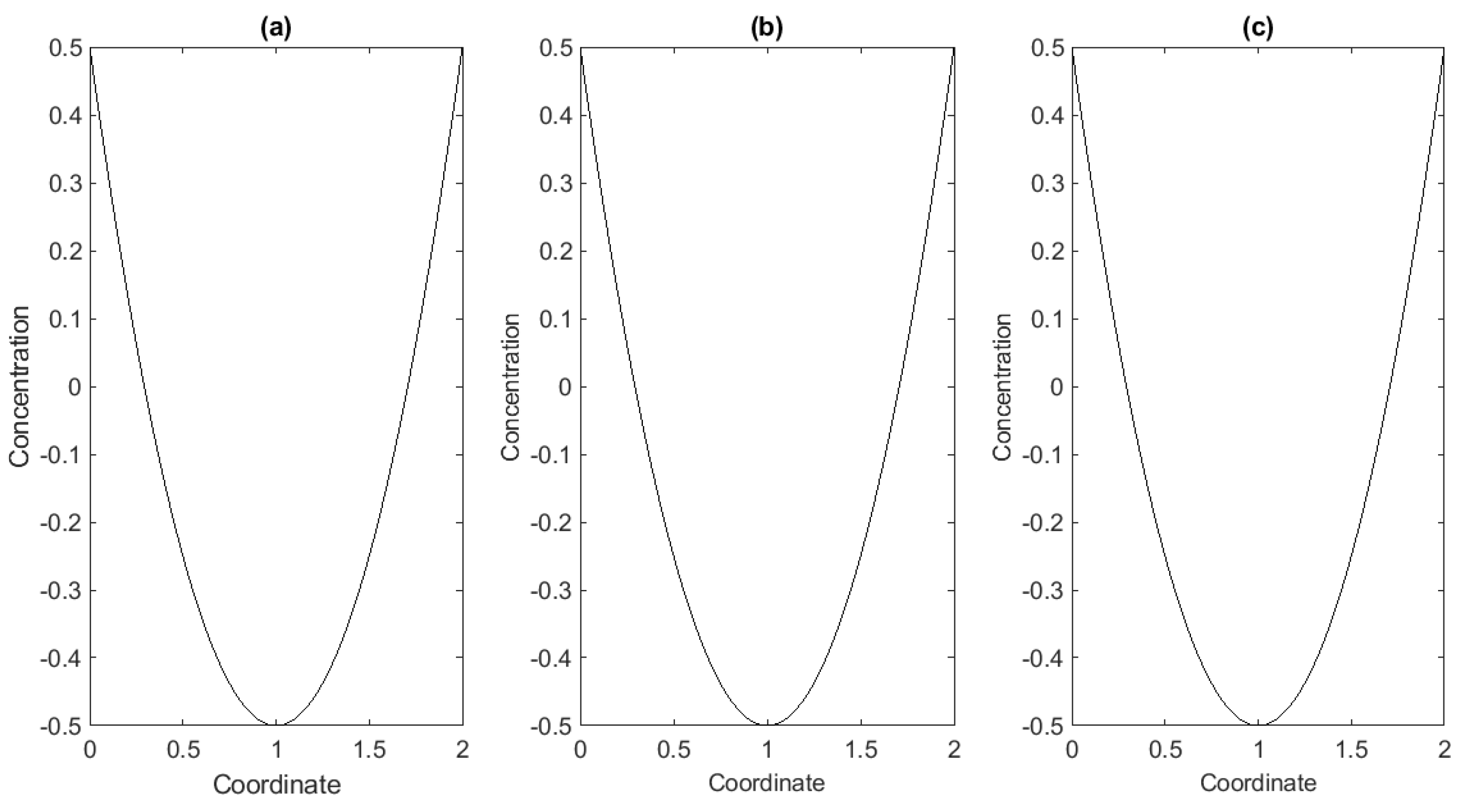
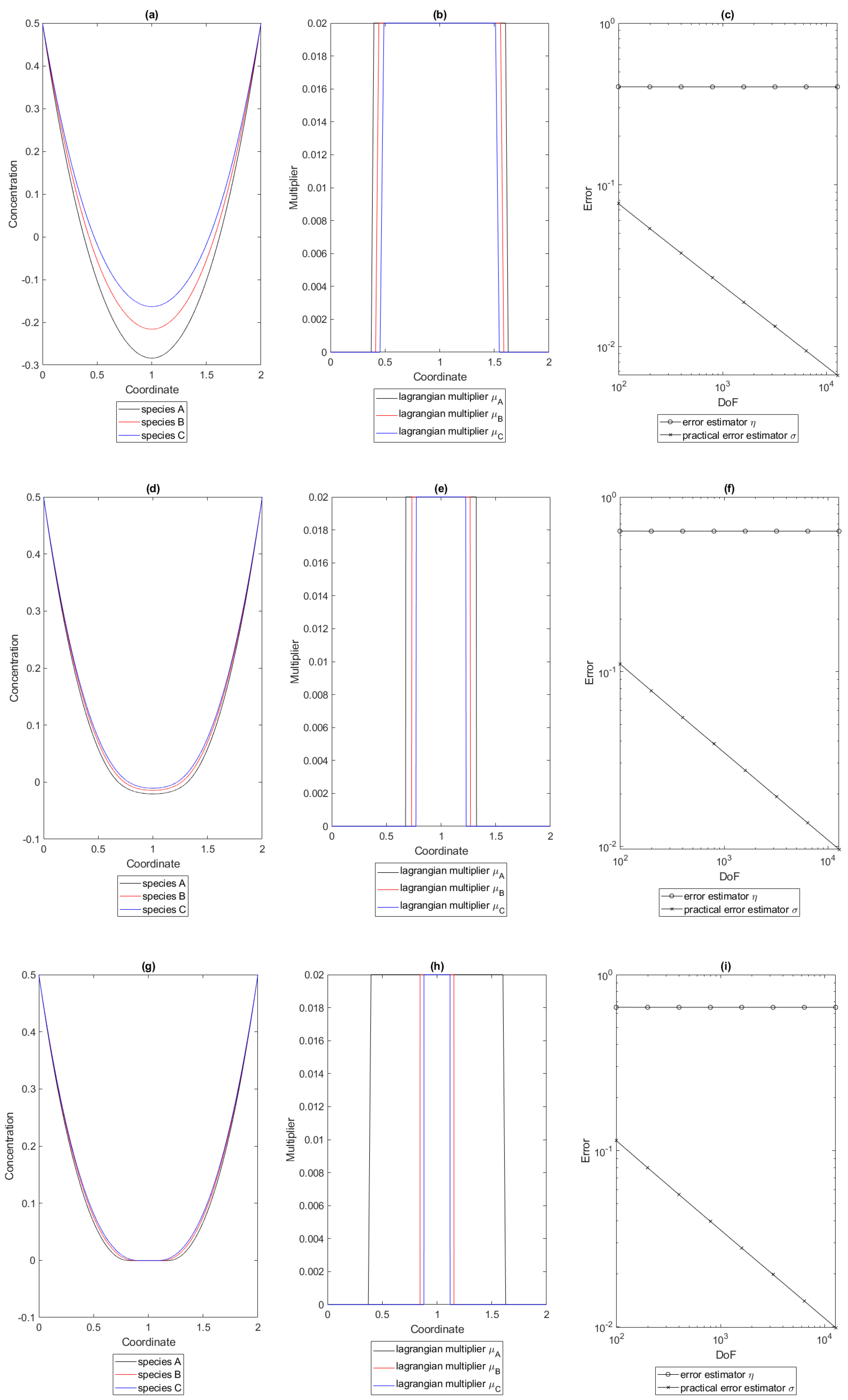
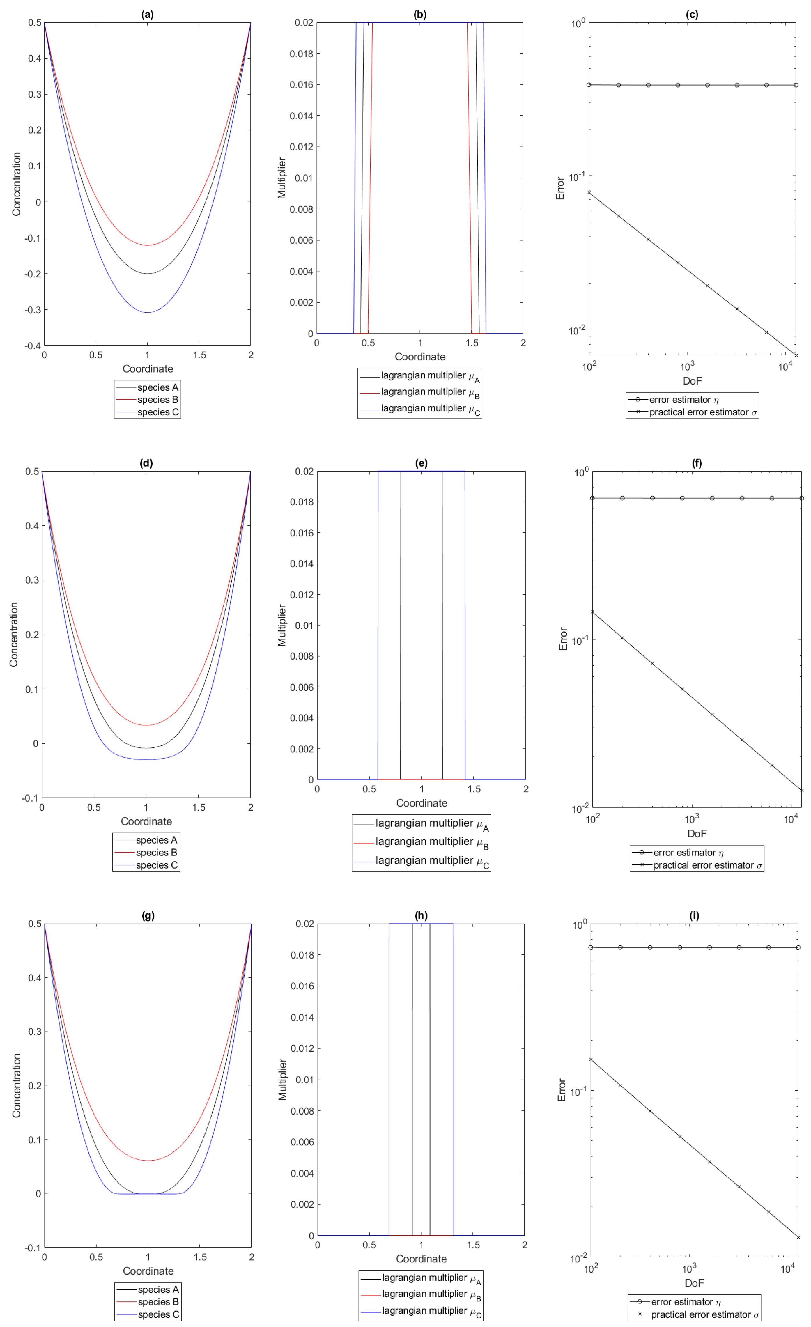
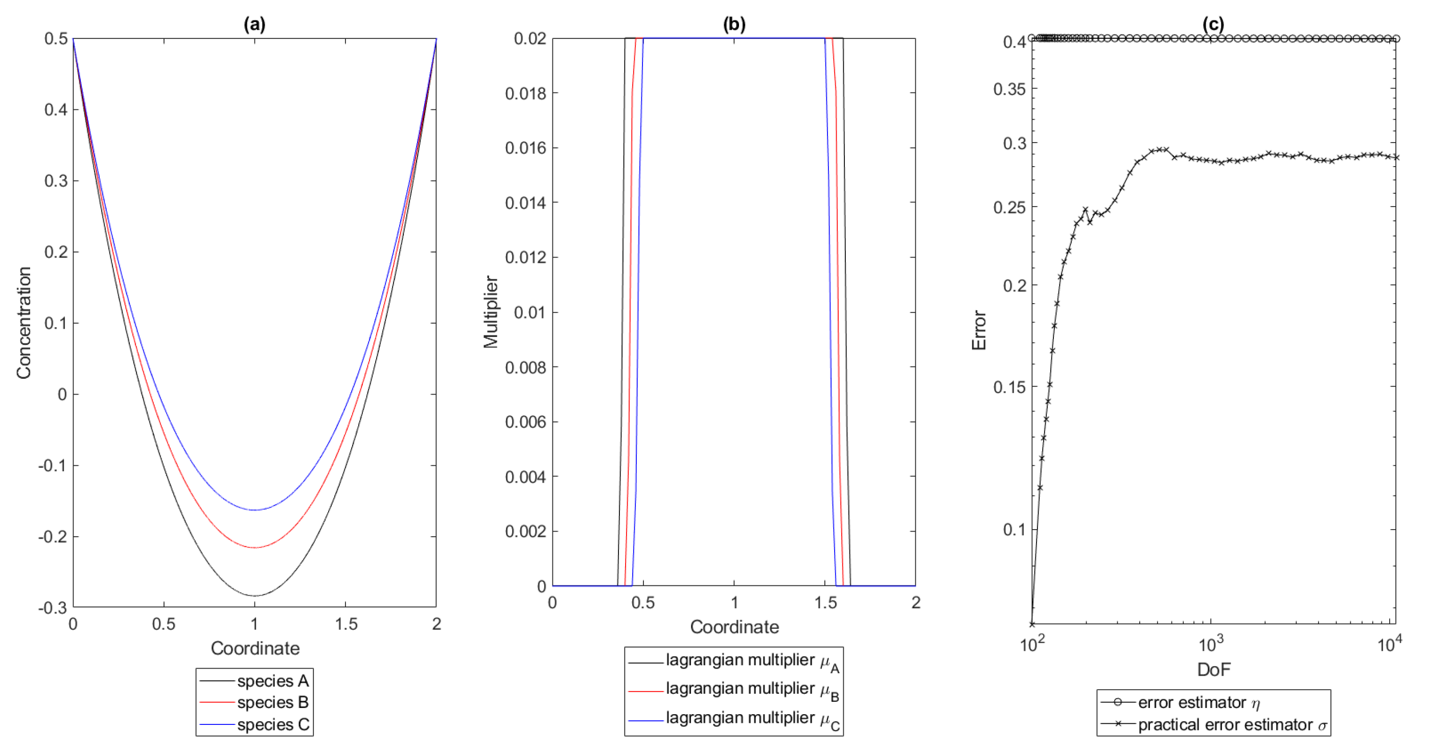
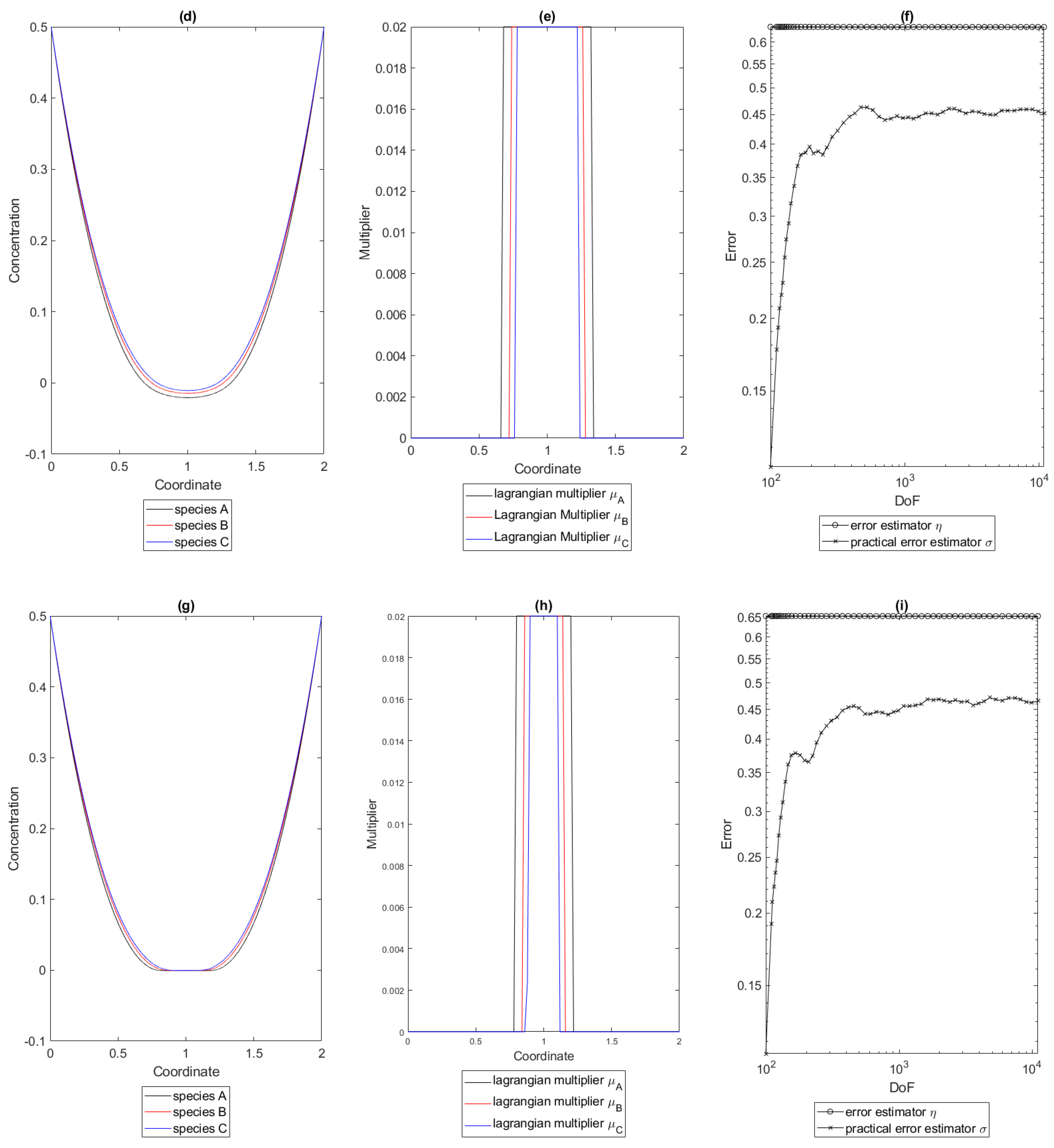
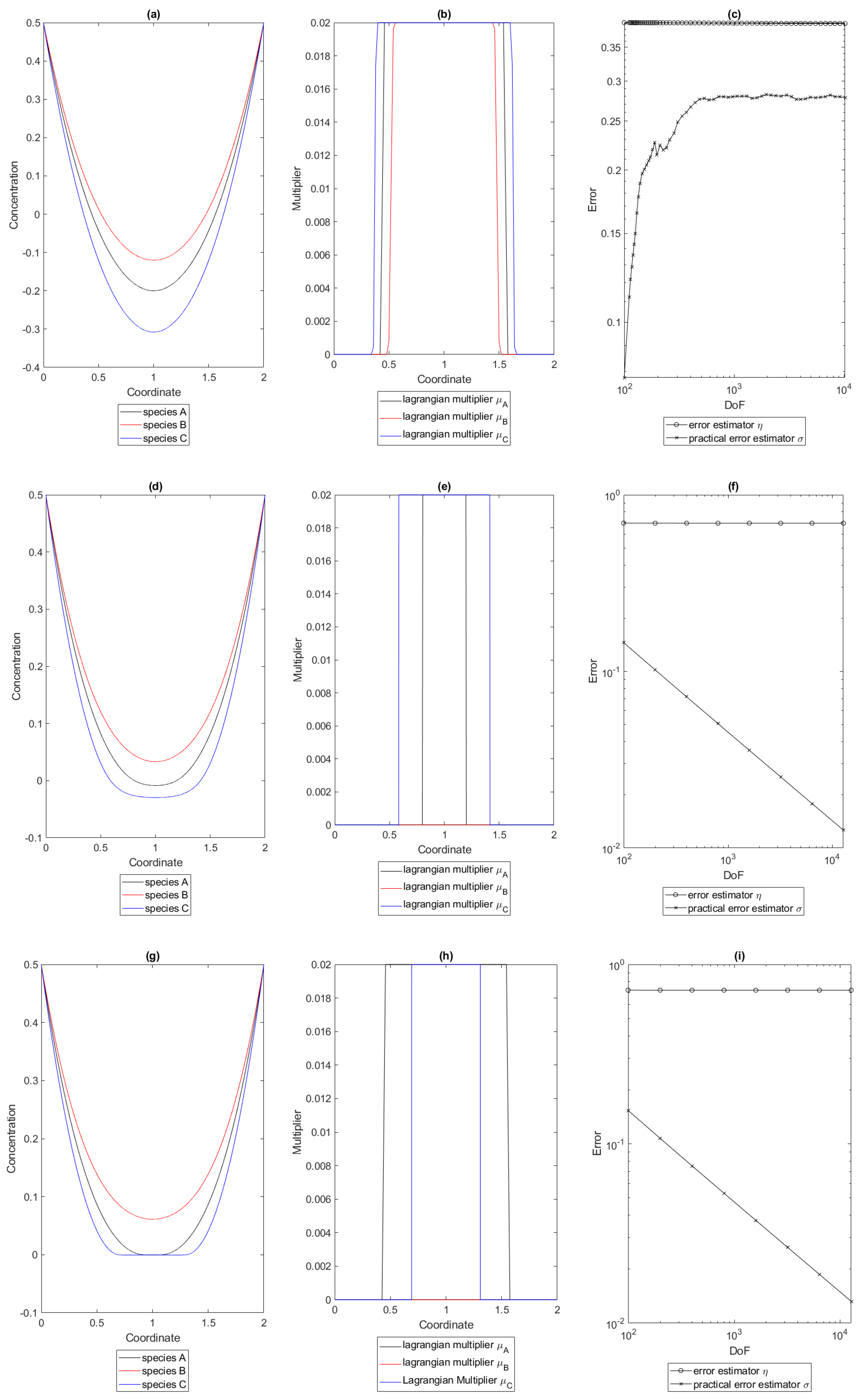
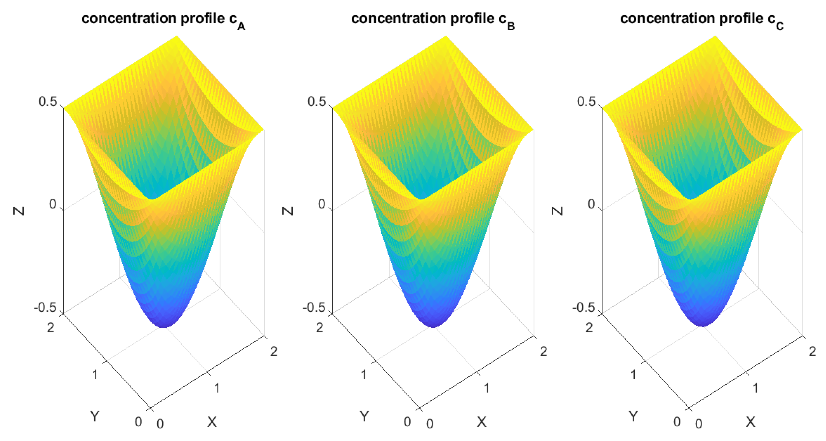
4.1. Numerical Examples in 1d
- The breaking condition from S3 in Algorithm 1 is fulfilled with a tolerance .
- The number of nodes in the current mesh increases nodes.
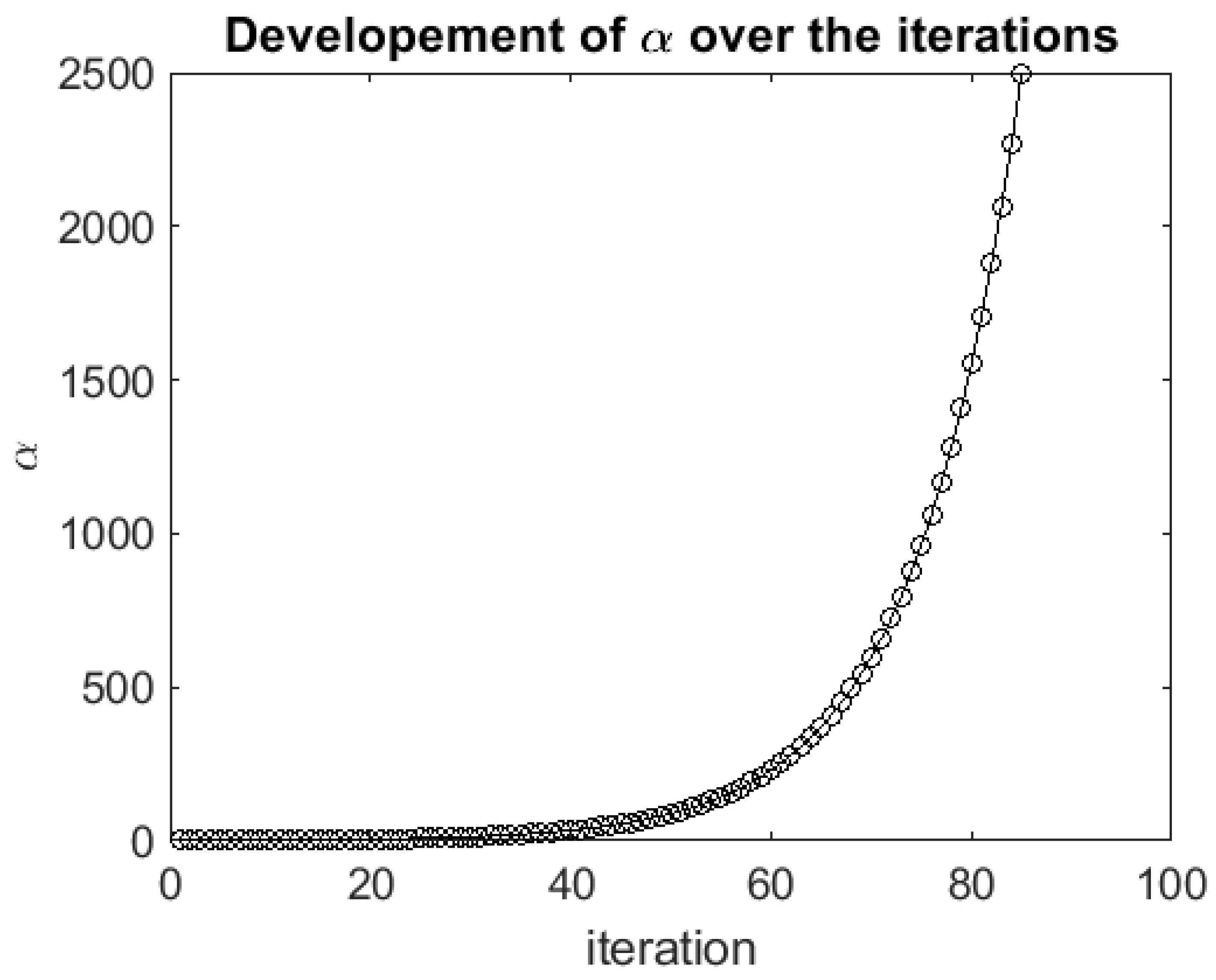
- More than 100,000 iterations of the augmented Lagrangian algorithm were performed.
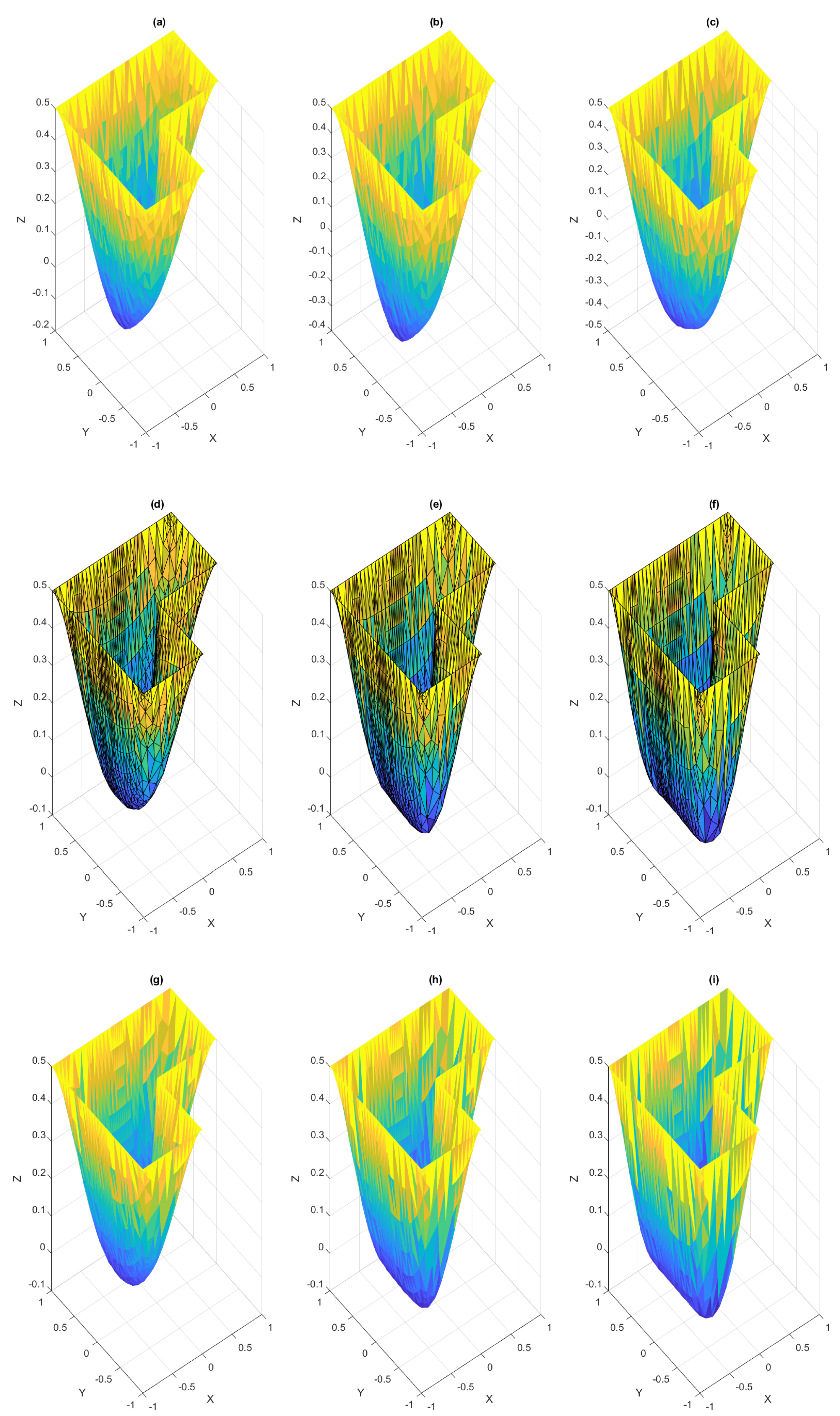
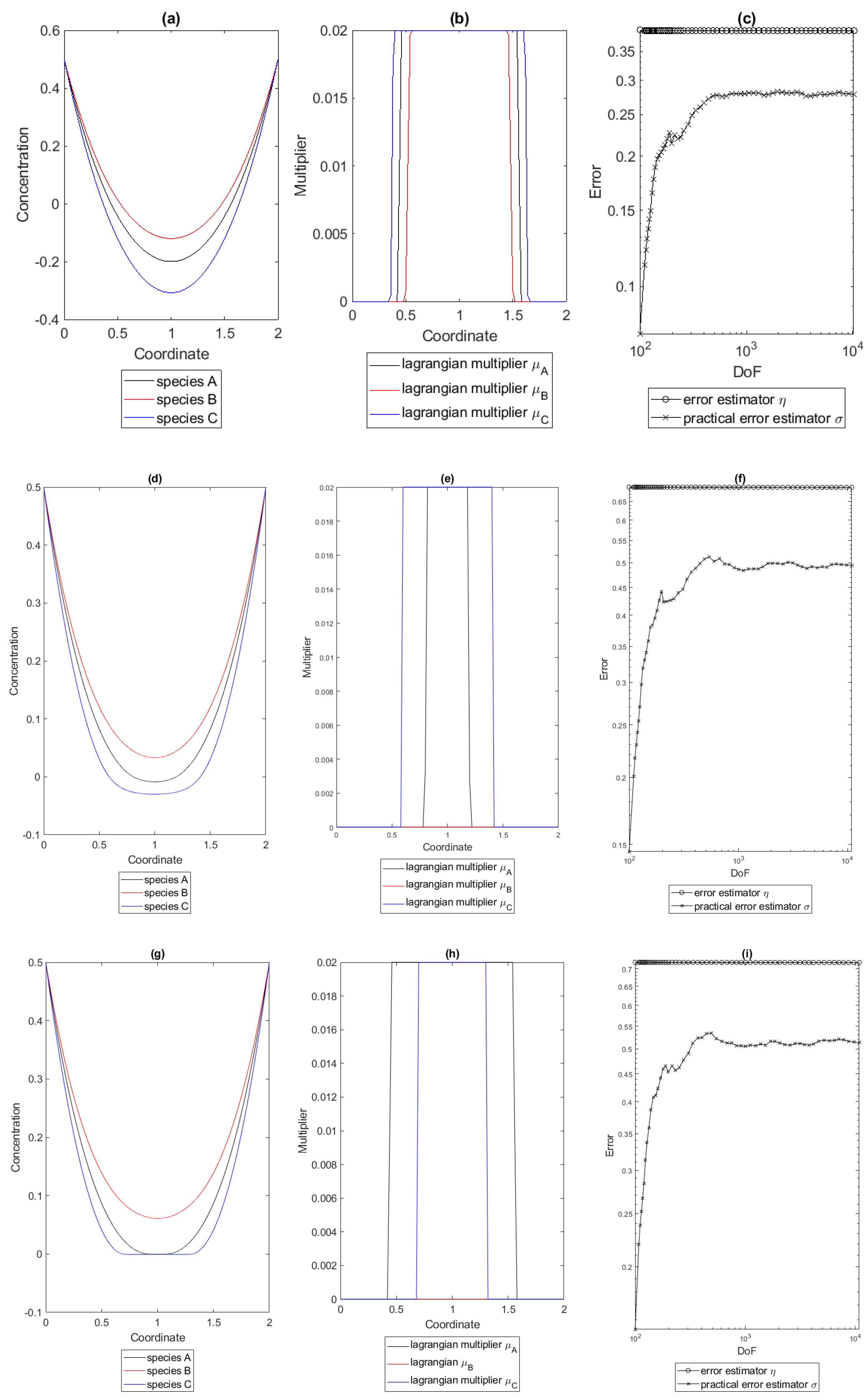
4.2. Examples in 2d
- The breaking condition from S3 in Algorithm 1 is fulfilled with a tolerance .
- The number of nodes in the current mesh increases 1000 nodes.
- More than 100,000 iterations of the augmented Lagrangian algorithm were performed.
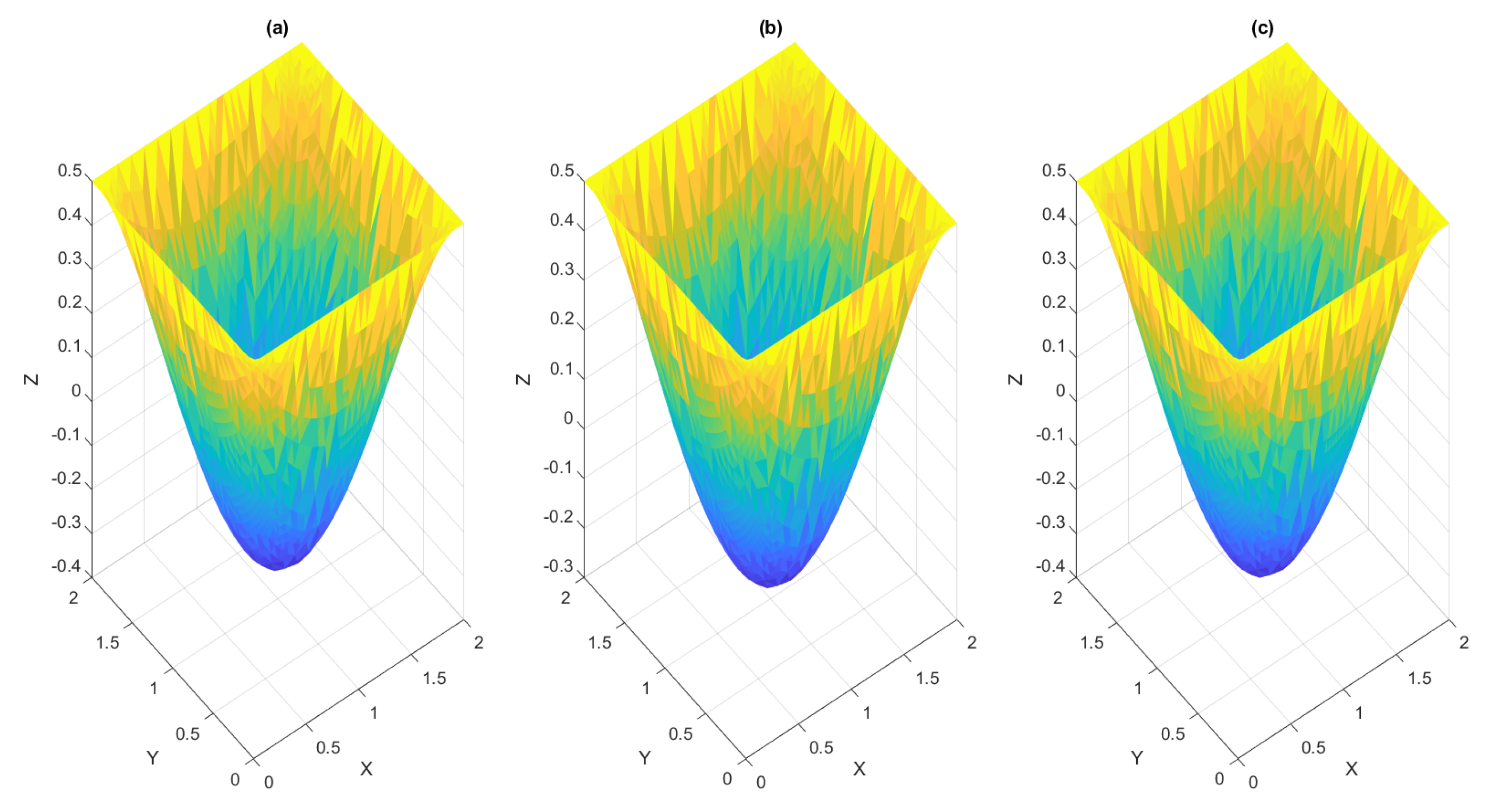
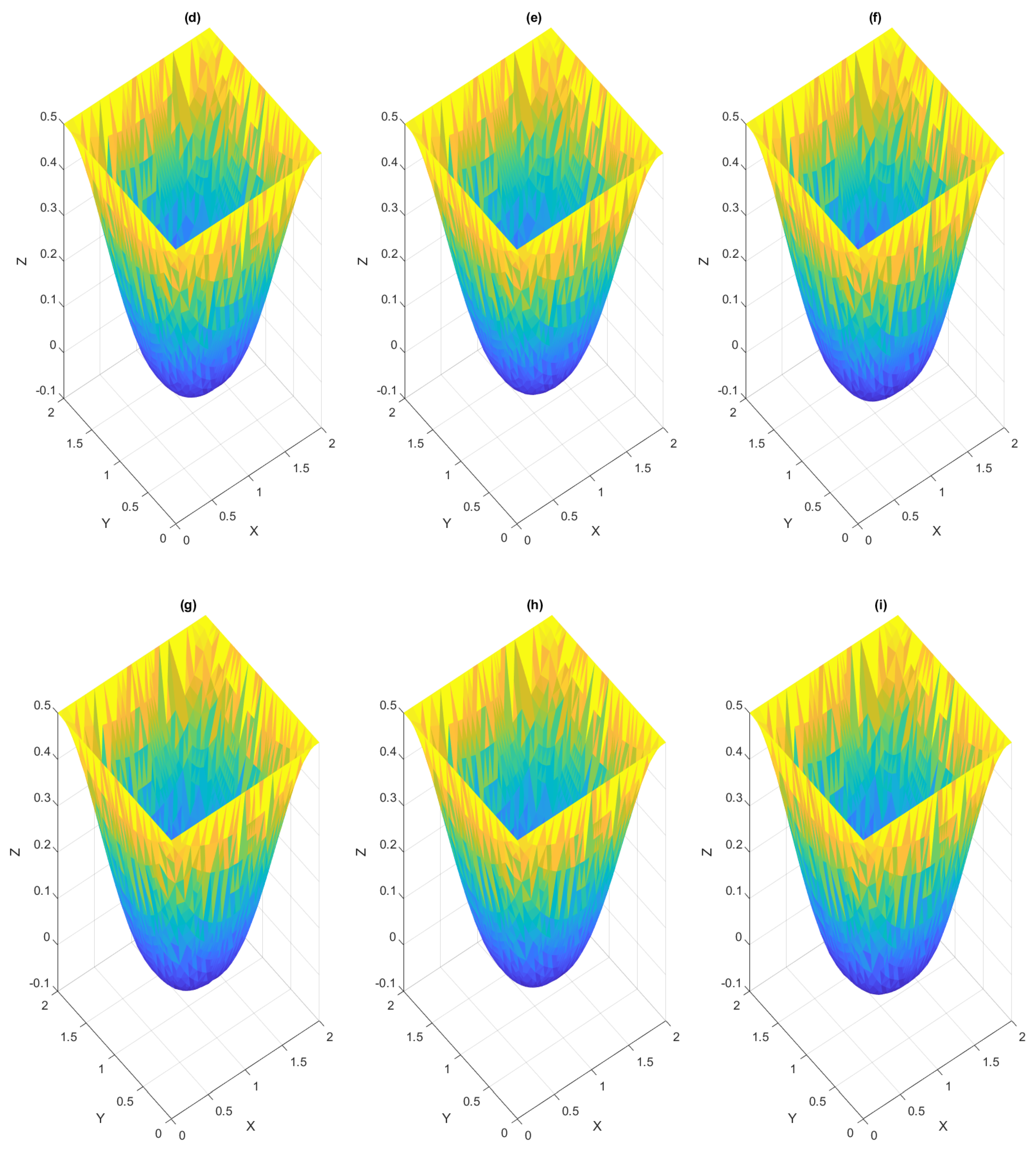
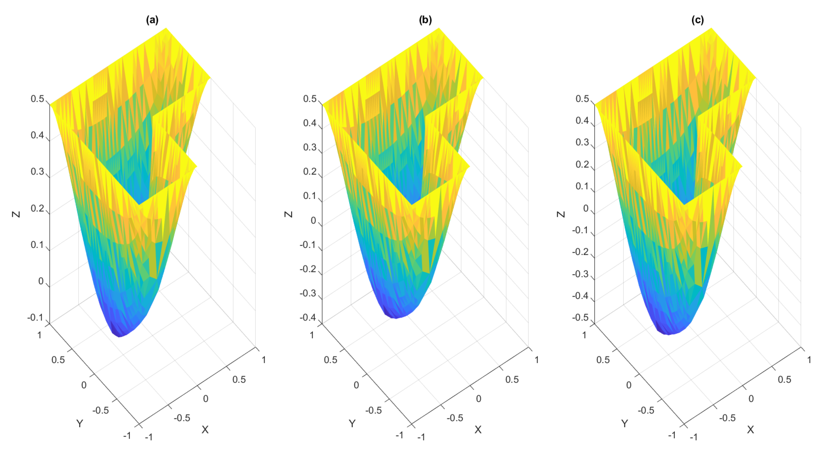
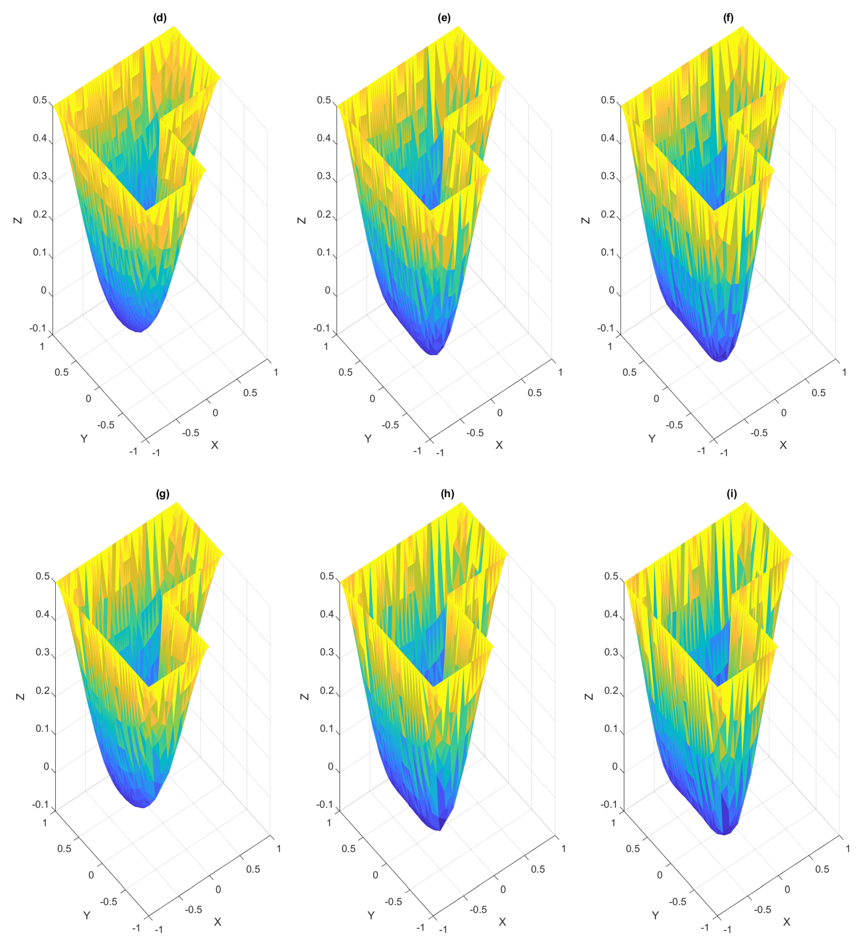
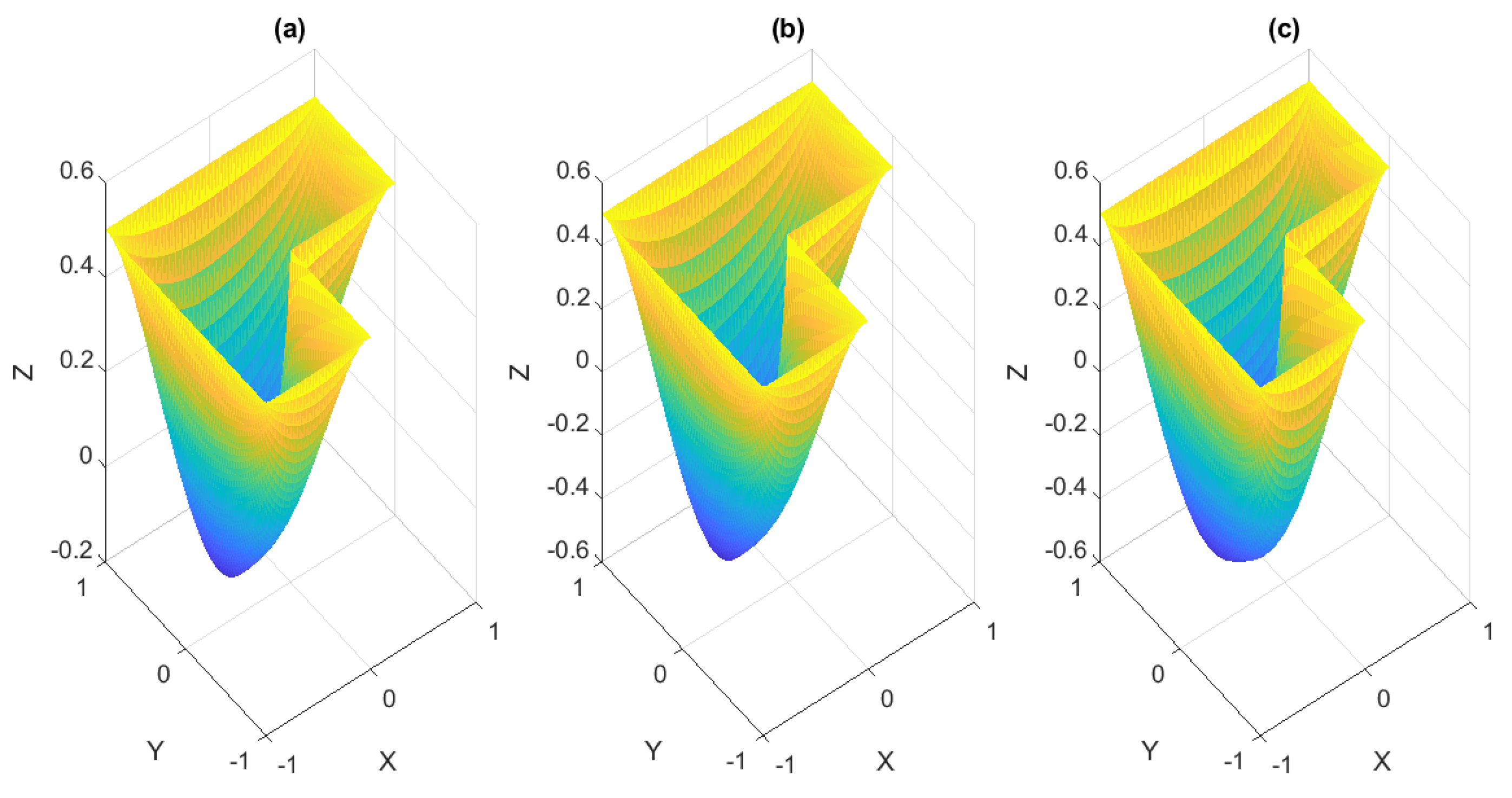
4.2.1. Examples on a Convex Domain
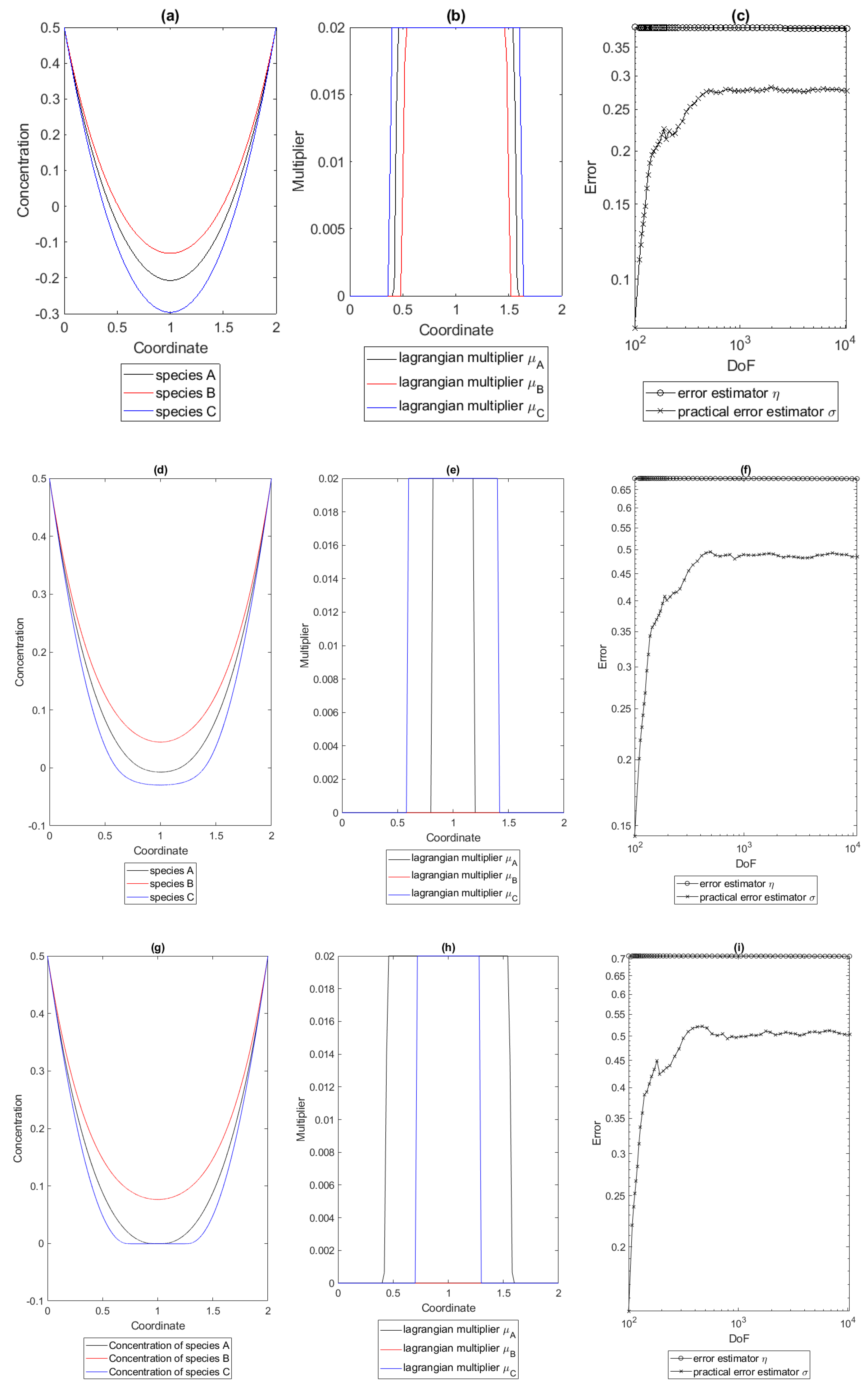
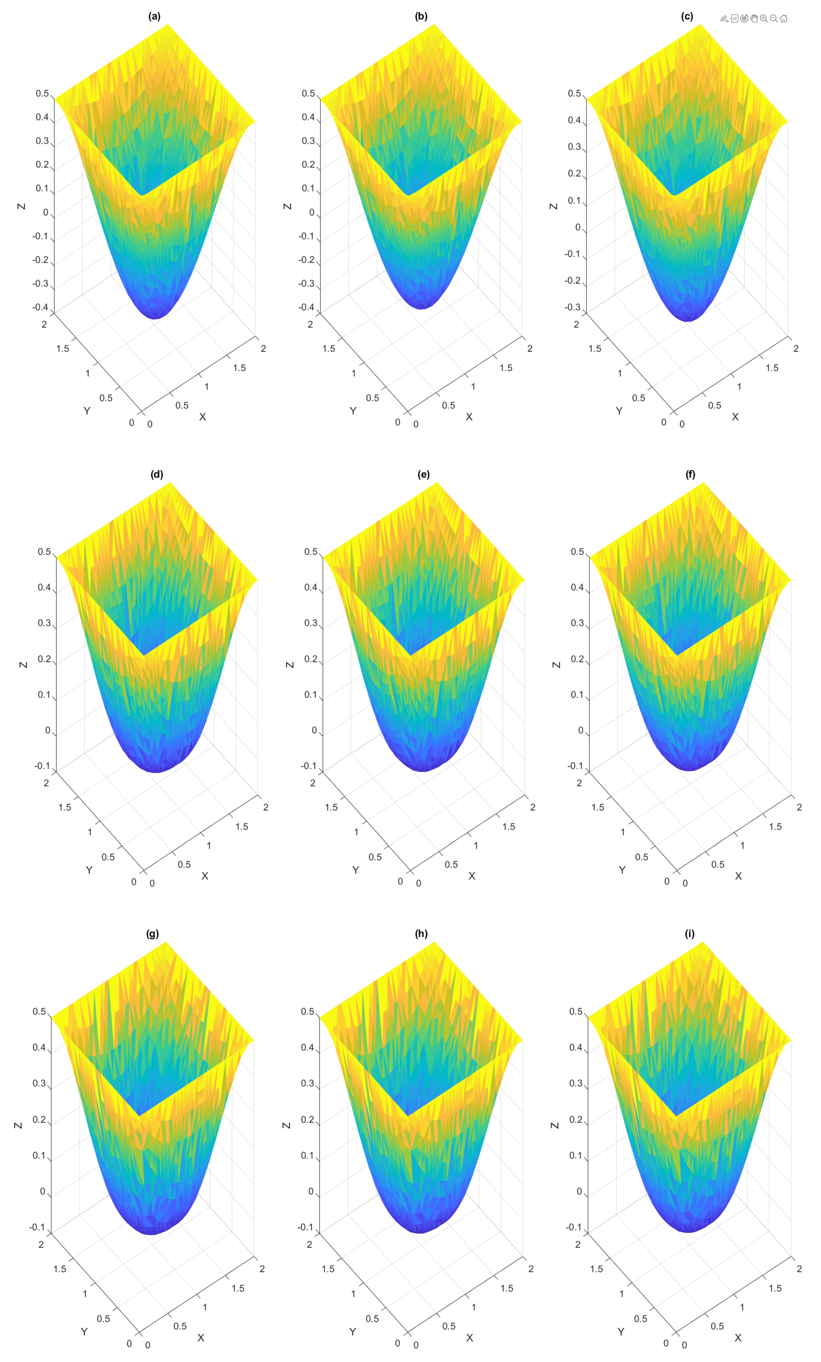
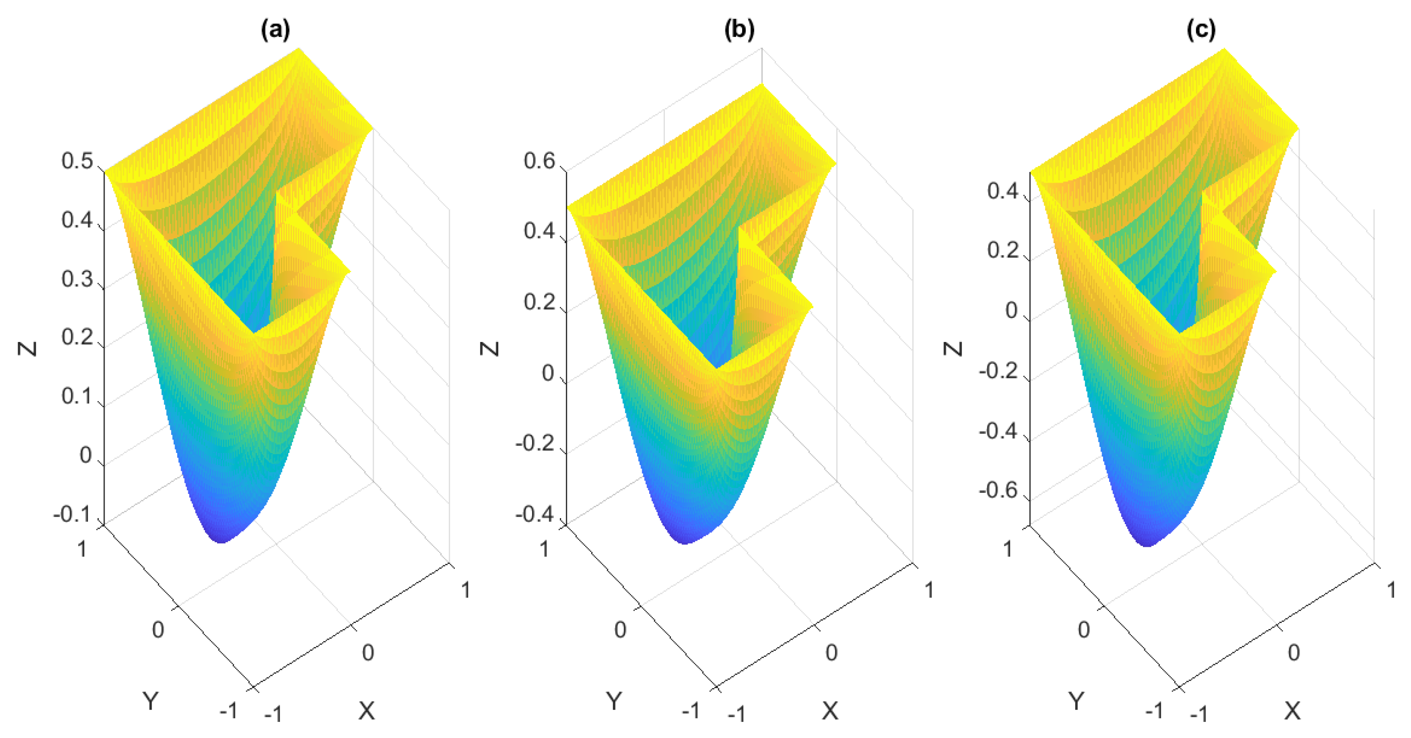
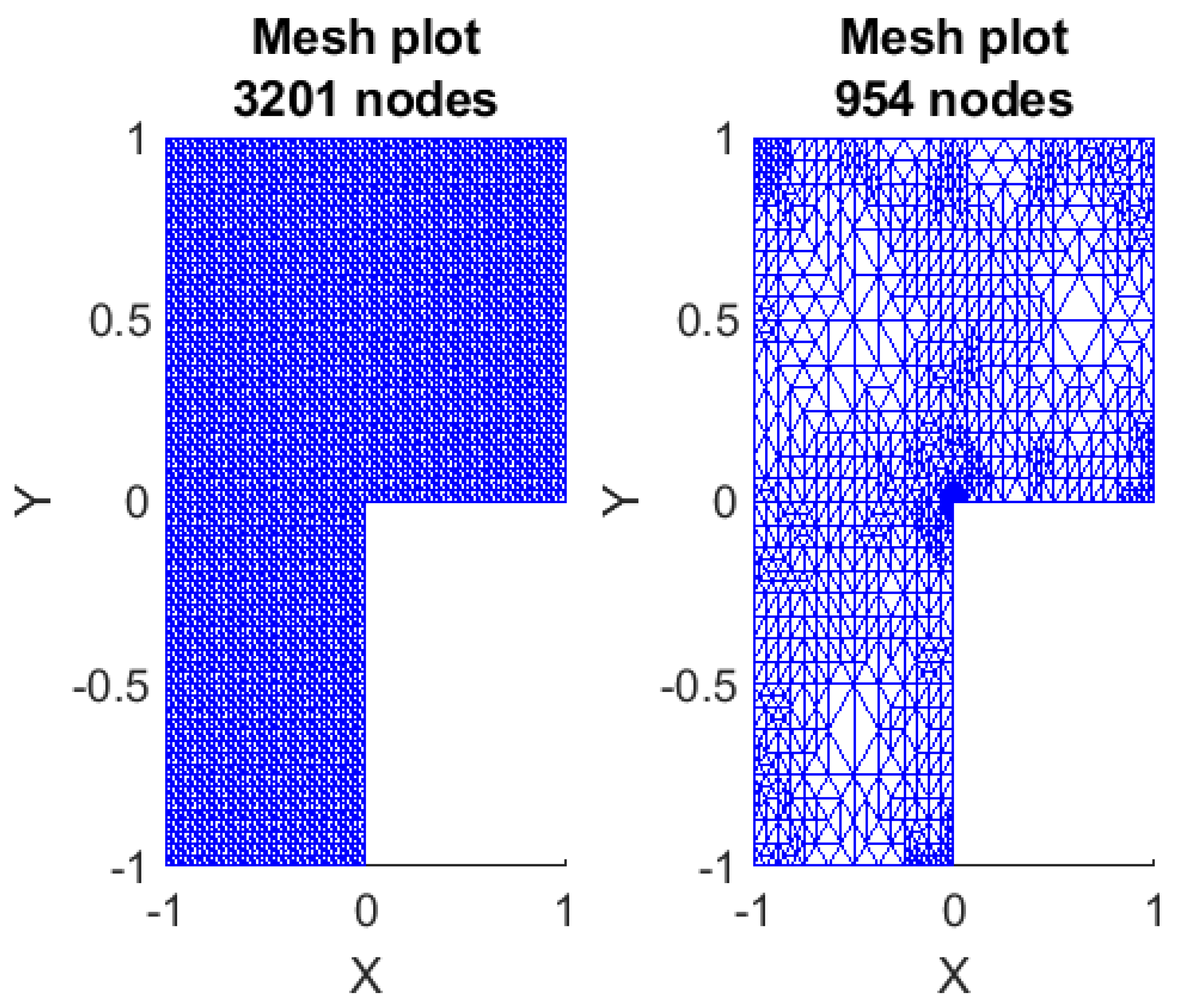
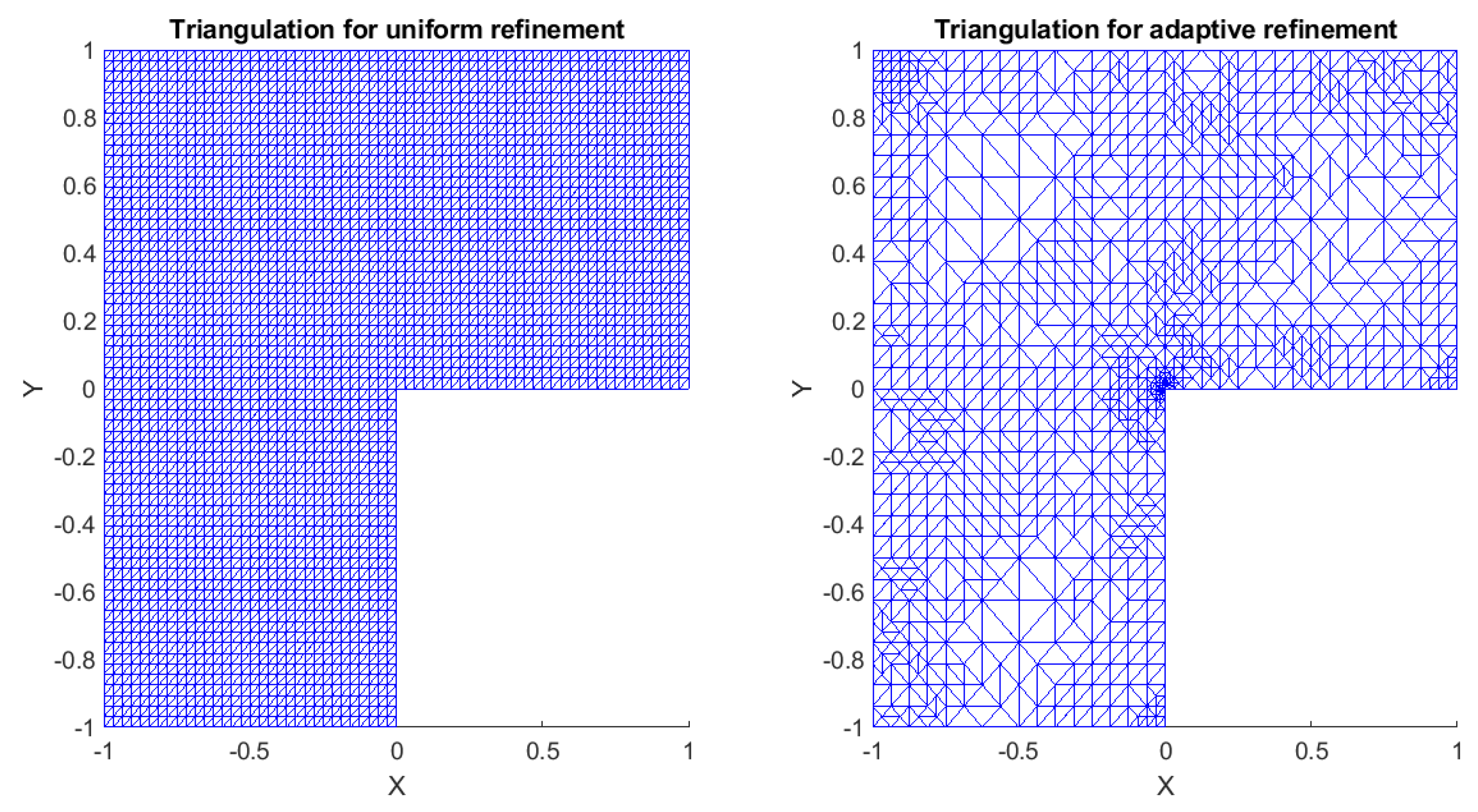
4.2.2. Examples on a Non-Convex Domain
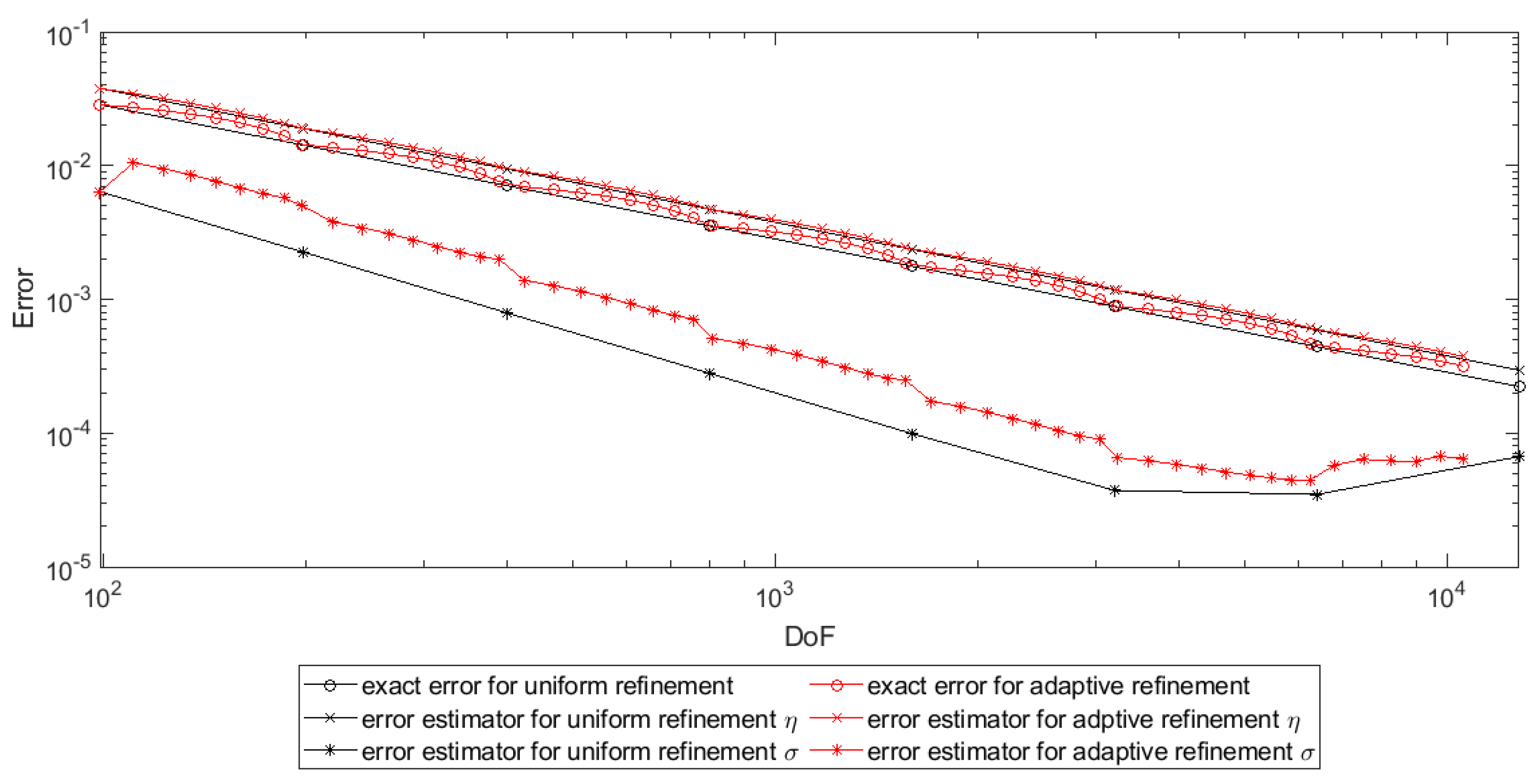
4.3. Comparison to Other Methods
4.3.1. Theoretical Setup for the Classical Augmented Lagrangian Scheme and the Primal-Dual Active-Set Strategy
4.3.2. Description Classical Augmented Lagrangian Regime
| Algorithm 4: Classical augmented Lagrangian method |
| Input: Define a starting values , , and define . Output: Approximate solution to (33) and approximate Lagrangian function . The classical augmented Lagrangian algorithm is given through the following steps.
|
| Algorithm 5: Refinement strategy with the classical augmented Lagrangian algorithm |
| Input: Initial Triangulation . Define a starting values , , and define . Output: Approximate solution to (33) and approximate Lagrangian function and final triangulation . Perform the following steps:
|
4.3.3. Description of the Primal-Dual Active-Set Strategy
| Algorithm 6: Primal-Dual Active-Set Strategy |
| Input: Define a starting values , , and define . Output: Approximate solution to (33) and approximate Lagrangian function . With the notation above the Primal-Dual Active-Set Strategy for this problem type
|
| Algorithm 7: Primal-Dual Active-Set strategy with refinement strategy |
| Input: Define a starting values , , and define . Furthermore define an initial triangulation . Output: Approximate solution to (33) and approximate Lagrangian function . Additionally the algorithm outputs the final triangulation Perform the following steps:
|
4.3.4. Comparrison of the Different Mehtods
5. Modelling the Stationary Species Transport in the Diffusion-Boundary Layer during the Metal Deposition from a Electrolyte
5.1. Theoretical Model
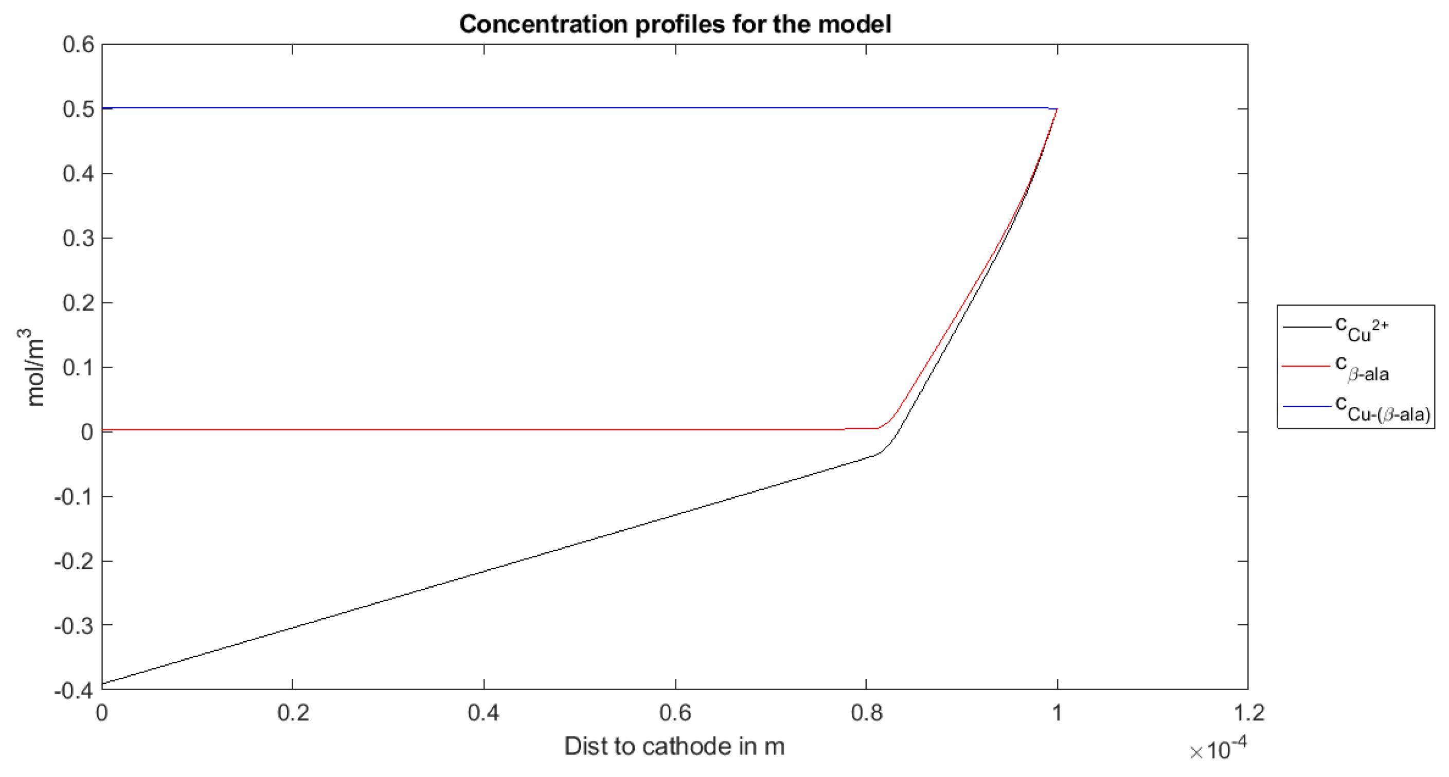
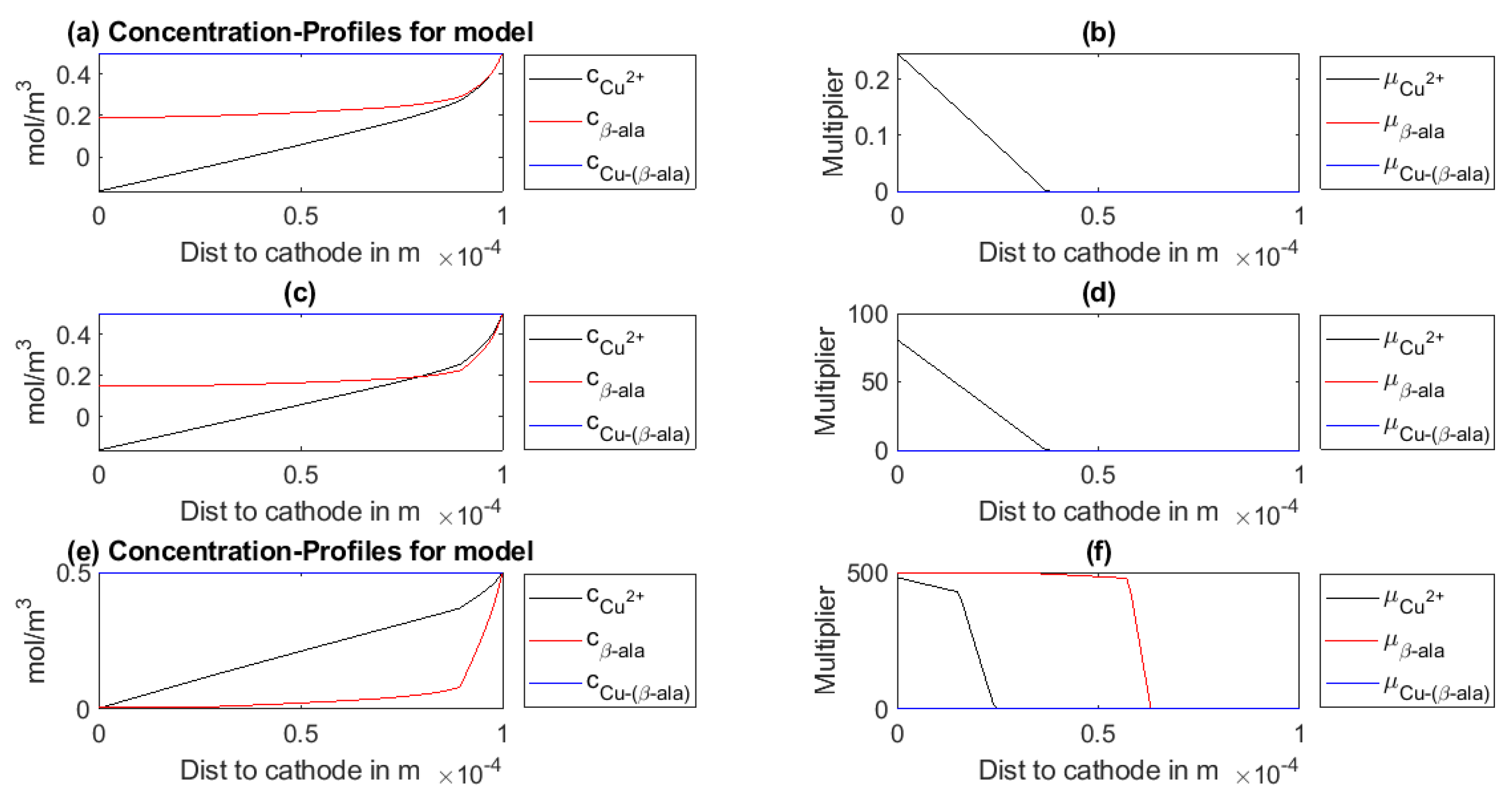
5.2. Simulation
6. Discussion and Conclusions
Author Contributions
Funding
Institutional Review Board Statement
Informed Consent Statement
Conflicts of Interest
Abbreviations
| PDE | Partial Differential Equation |
| ODE | Ordenary Differential Equation |
| FEM | Finite Element Method |
| s.t. | subject to |
| DoF | Degree of Freedom |
| RHS | right hand side |
| w.r.t. | with respect to |
References
- Newman, J.S. Electrochemical Systems, 2nd ed.; Prentice-Hall International Series in the Physical and Chemical Engineering Sciences; Prentice Hall: Upper Saddle River, NJ, USA, 1991. [Google Scholar]
- Bard, A.; Faulkner, L. (Eds.) Electrochemical Methods: Fundamentals and Applications; John Wiley & Sons, Ltd.: New York, NY, USA; Chichester, UK; Weinheim, Germany; Brisbane, Australia; Singapore; Toronto, ON, Canada, 1980; Volume 18. [Google Scholar]
- Survila, A. Electrochemistry of Metal Complexes; John Wiley & Sons, Ltd.: Hoboken, NJ, USA, 2015; Chapter 3; pp. 33–59. [Google Scholar] [CrossRef]
- Buffle, J.; Zhang, Z.; Startchev, K. Metal Flux and Dynamic Speciation at (Bio)interfaces. Part I: Critical Evaluation and Compilation of Physicochemical Parameters for Complexes with Simple Ligands and Fulvic/Humic Substances. Environ. Sci. Technol. 2007, 41, 7609–7620. [Google Scholar] [CrossRef] [PubMed]
- Averós, J.; Llorens, J.; Uribe-Kaffure, R. Numerical simulation of non-linear models of reaction-diffusion for a DGT sensor. Algorithms 2020, 13, 98. [Google Scholar] [CrossRef] [Green Version]
- Mongin, S.; Uribe, R.; Puy, J.; Cecília, J.; Galceran, J.; Zhang, H.; Davison, W. Key Role of the Resin Layer Thickness in the Lability of Complexes Measured by DGT. Environ. Sci. Technol. 2011, 45, 4869–4875. [Google Scholar] [CrossRef] [PubMed]
- Zeidler, E. Nichtlineare partielle Differentialgleichungen. In Springer-Handbuch der Mathematik IV: Begründet von I.N. Bronstein und K.A. Semendjaew Weitergeführt von G. Grosche, V. Ziegler und D. Ziegler Herausgegeben von E. Zeidler; Zeidler, E., Ed.; Springer Fachmedien Wiesbaden: Wiesbaden, Germany, 2013; pp. 311–356. [Google Scholar] [CrossRef]
- Schinagl, K. Numerische Simulation von chemischen Reaktionen in Flüssigkeiten. Ph.D. Thesis, Rheinische Friedrich-Wilhelms-Universität Bonn, Bonn, Germany, 2013. [Google Scholar]
- Roland, M. Numerische Simulation von Fällungsprozessen mittels Populationsbilanzen. Ph.D. Thesis, Universität des Saarlandes, Saarbrücken, Germany, 2010. [Google Scholar]
- Chen, J.; Wang, H.; Liew, K.; Shen, S. A Fully Coupled Chemomechanical Formulation with Chemical Reaction Implemented by Finite Element Method. J. Appl. Mech. Trans. ASME 2019, 86. [Google Scholar] [CrossRef]
- Rodrigues, J. Obstacle Problems in Mathematical Physics; Elsevier: Amsterdam, The Netherlands, 1987. [Google Scholar]
- Shillor, M.; Sofonea, M.; Telega, J.J. 11 Contact with Wear or Adhesion. In Models and Analysis of Quasistatic Contact: Variational Methods; Springer: Berlin/Heidelberg, Germany, 2004; pp. 183–206. [Google Scholar] [CrossRef]
- Laursen, T.A. Finite Element Implementation of Contact Interaction. In Computational Contact and Impact Mechanics: Fundamentals of Modeling Interfacial Phenomena in Nonlinear Finite Element Analysis; Springer: Berlin/Heidelberg, Germany, 2003; pp. 145–209. [Google Scholar] [CrossRef]
- Brezzi, F.; Hager, W.; Hager, P. Error Estimates for the Finite Element Solution of Variational Inequalities. Numer. Math. 1977, 28, 431–443. [Google Scholar] [CrossRef]
- Wang, L.H. On the quadratic finite element approximation to the obstacle problem. Numer. Math. 2002, 92, 771–778. [Google Scholar] [CrossRef]
- Hinze, P.; Pimau, R.; Ulbrich, M.; Ulbrich, S. Optimization with PDE Constraints, 1st ed.; Mathematical Modelling: Theory and Applications; Springer Netherlands: Dordrecht, The Netherlands, 2009; Volume 23. [Google Scholar]
- Mäkelä, M.M.; Neittaanmäki, P. NONSMOOTH OPTIMIZATION-Analysis and Algorithms with Applications to Optimal Control, 1st ed.; World Scientific Publishing Co. Pte. Ltd.: Singapore, 1992. [Google Scholar]
- Byrd, R.H.; Gilbert, J.C.; Nocedal, J. A trust region method based on interior point techniques for nonlinear programming. Math. Program. 2000, 89, 149–185. [Google Scholar] [CrossRef] [Green Version]
- Glowinski, R. Numerical Methods for Nonlinear Variational Problems; Springer: Berlin/Heidelberg, Germany, 2008. [Google Scholar]
- Antipin, A.; Vasilieva, O. Augmented Lagrangian Method for Optimal Control Problems. In Analysis, Modelling, Optimization, and Numerical Techniques; Tost, G.O., Vasilieva, O., Eds.; Springer International Publishing: Cham, Switzerland, 2015; pp. 1–36. [Google Scholar]
- Ito, K.; Kunisch, K. The augmented lagrangian method for equality and inequality constraints in hilbert spaces. Math. Program. 1990, 46, 341–360. [Google Scholar] [CrossRef]
- Andrei, N. Penalty and Augmented Lagrangian Methods. In Continuous Nonlinear Optimization for Engineering Applications in GAMS Technology; Springer International Publishing: Cham, Switzerland, 2017; pp. 185–201. [Google Scholar] [CrossRef]
- Hintermüller, M.; Ito, K.; Kunisch, K. The primal-dual active set strategy as a semismooth Newton Method. SIAM J. Optim. 2003, 13, 865–888. [Google Scholar] [CrossRef] [Green Version]
- Carstensen, C.; Feischl, M.; Page, M.; Praetorius, D. Axioms of adaptivity. ELSVIER, Comput. Math. Appl. 2014, 67, 1195–1253. [Google Scholar] [CrossRef] [PubMed] [Green Version]
- Kanzow, C.; Steck, D.; Wachsmuth, D. An Augmented Lagrangian Method for Optimization Problems in Banach Spaces. SIAM J. Control Optim. 2018, 56, 272–291. [Google Scholar] [CrossRef]
- Steck, D. Lagrange Multiplier Methods for Constrained Optimization and Variational Problems in Banach Spaces. Ph.D. Thesis, Universität Würzburg, Würzburg, Germany, 2018. [Google Scholar]
- Grossmann, C.; Roos, H.G.; Stynes, M. Numerical Treatment of Partial Differential Equations; Springer: Berlin/Heidelberg, Germany, 2007. [Google Scholar]
- Bochev, P.B.; Gunzburger, D. Least-Squares Finite Element Methods; Applied Mathematical Sciences; Springer: New York, NY, USA, 2009; Volume 166. [Google Scholar]
- Boffi, D.; Brezzi, F.; Fortin, M. Mixed Finite Element Methods and Applications; Springer: Berlin/Heidelberg, Germany, 2013. [Google Scholar]
- Braess, D. Finite Elemente, 5th ed.; Theorie, Schnelle Löser und Anwendungen in der Elastizitätstheorie; Springer: Heidelberg, Germany, 2012. [Google Scholar]
- Li, T.Y. Homotopy Methods. In Encyclopedia of Applied and Computational Mathematics; Engquist, B., Ed.; Springer: Berlin/Heidelberg, Germany, 2015; pp. 653–656. [Google Scholar] [CrossRef]
- Watson, L.T. Globally convergent homotopy methodsGlobally Convergent Homotopy Methods. In Encyclopedia of Optimization; Floudas, C.A., Pardalos, P.M., Eds.; Springer: Boston, MA, USA, 2009; pp. 1272–1277. [Google Scholar] [CrossRef]
- Evans, L. Partial Differential Equations; Graduate Studies in Mathematics; AMS: Providence, RI, USA, 1997; Volume 166. [Google Scholar]
- Tadmor, E. A review of numerical methods for nonlinear partial differential equations. Bull. Am. Math. Soc. 2012, 49, 507–554. [Google Scholar] [CrossRef] [Green Version]
- Grüne, L.; Junge, O. Gewöhnliche Differentialgleichungen, Eine Einführung aus der Perspektive der Dynamischen Systeme; Springer Spectrum: Wiesbaden, Germany, 2016; Volume 2. [Google Scholar]
- Attouch, H.; Buttazzo, G.; Michaille, G. Variational Analysis in Sobolev and BV Spaces; Society for Industrial and Applied Mathematics: Philadelphia, PA, USA, 2014. [Google Scholar] [CrossRef]
- Braides, A. A Handbook of Γ-Convergence. Stationary Partial Differential Equations; Chipot, P., Quittner, P., Eds.; Elsevier: Amsterdam, The Netherlands, 2006; Volume 3. [Google Scholar]
- DalMaso, G. An Introduction to Γ-Convergence; Birkhäuser Boston Inc.: Boston, MA, USA, 1993. [Google Scholar]
- Braides, A.; Defranceschi, A. Homogenization of Multiple Integrals; Oxford University Press, Inc.: New York, NY, USA, 1998. [Google Scholar]
- Alt, H.W. Lineare Funktionalanalysis, 6th ed.; Springer: Heidelberg, Germany, 2012. [Google Scholar]
- Zeidler, E. Variationsrechnung und Physik. In Springer-Handbuch der Mathematik III: Begründet von I.N. Bronstein und K.A. Semendjaew Weitergeführt von G. Grosche, V. Ziegler und D. Ziegler Herausgegeben von E. Zeidler; Zeidler, E., Ed.; Springer Fachmedien Wiesbaden: Wiesbaden, Germany, 2013; pp. 1–48. [Google Scholar] [CrossRef]
- Crank, J.; Nicolson, P. A practical method for numerical evaluation of solutions of partial differential equations of the heat-conduction type. Math. Proc. Camb. Philos. Soc. 1947, 43, 50–67. [Google Scholar] [CrossRef]
- Evans, G.A.; Blackledge, J.M.; Yardley, P.D. Finite Element Method for Ordinary Differential Equations. In Numerical Methods for Partial Differential Equations; Springer: London, UK, 2000; pp. 123–164. [Google Scholar] [CrossRef]
- Rockafellar, R.T. Convex Analysis; Princeton University Press: Princeton, NJ, USA, 2015. [Google Scholar]
- Polak, E. Unconstrained Optimization. In Optimization: Algorithms and Consistent Approximations; Springer: New York, NY, USA, 1997; pp. 1–166. [Google Scholar] [CrossRef]
- Lange, K. Optimization, 2nd ed.; Springer Texts in Statistics; Springer: New York, NY, USA, 2013. [Google Scholar]
- Carstensen, C.; Rabus, H. Axioms of adaptivity with separate marking for data resolution. SIAM J. Numer. Anal. 2017, 55, 2644–2665. [Google Scholar] [CrossRef]
- Traxler, C. An algorithm for adaptive mesh refinement in n dimensions. Computing 1997, 59, 115–137. [Google Scholar] [CrossRef]
- Dörfler, W. A Convergent Adaptive Algorithm for Poisson’s Equation. SIAM J. Numer. Anal. 1996, 33, 1106–1124. [Google Scholar] [CrossRef]
- Carstensen, C.; Park, E.J. Convergence and Optimality of Adaptive Least Squares Finite Element Methods. SIAM J. Numer. Anal. 2015, 53, 43–62. [Google Scholar] [CrossRef]
- Hellwig, F. Adaptive Discontinuous Petrov-Galerkin Finite-Element-Methods. Ph.D. Thesis, Humboldt-Universität zu Berlin, Mathematisch-Naturwissenschaftliche Fakultät, Berlin, Germany, 2019. [Google Scholar] [CrossRef]
- Carstensen, C.; Dond, A.K.; Nataraj, N.; Pani, A.K. Error analysis of nonconforming and mixed FEMs for second-order linear non-selfadjoint and indefinite elliptic problems. Numer. Math. 2016, 133, 557–597. [Google Scholar] [CrossRef] [Green Version]
- Ramm, A.G. A Simple Proof of the Fredholm Alternative and a Characterization of the Fredholm Operators. Am. Math. Mon. 2001, 108, 855–860. [Google Scholar] [CrossRef]
- Schatz, A. An Observation Concerning Ritz-Galerkin Methods with Indefinite Bilinear Forms. Math. Comput. 1974, 28, 959–962. [Google Scholar] [CrossRef]
- Hellwig, F. Software for PhD Thesis “Adaptive Discontinuous Petrov-Galerkin Finite-Element-Methods”. Ph.D. Thesis, Humboldt-Universität zu Berlin, Mathematisch-Naturwissenschaftliche Fakultät,, Berlin, Germany, 2019. [Google Scholar] [CrossRef]
- Oertel, H.J.; Böhle, M. Strömungsmechnanik-Grundlagen, Grundgleichungen, Lösungsmethoden, Softwarebeispiele, 3rd ed.; Studium Technik, Vieweg+Teubner Verlag: Wiesbaden, Germany, 2004. [Google Scholar] [CrossRef]
- Pluschke, V. Anwendung der Rothe-Methode auf eine quasilineare parabolische Differentialgleichung. Math. Nachr. 1983, 114, 105–121. [Google Scholar] [CrossRef]
- Gerdes, W. The initial boundary value problem for the threedimensional heat equation treated with Rothe’s line method using integral equations [Die Lösung des Anfangs-Randwertproblems für die Wärmeleitungsgleichung im R3 mit einer Integralgleichungs-methode nach dem Rotheverfahrenmit einer Integralgleichungs-methode nach dem Rotheverfahren]. Computing 1978, 19, 251–268. [Google Scholar] [CrossRef]


| Species | D in | in | in | |
|---|---|---|---|---|
| A | - | - | 0 | |
| B | - | - | 0 | |
| C | 0 | 0 | 0 |
| Species | D in | in | in | |
|---|---|---|---|---|
| A | - | - | 0 | |
| B | - | - | 0 | |
| C | 0 | 1 | 0 |
| Species | D in | in | in | |
|---|---|---|---|---|
| A | - | - | 0 | |
| B | - | - | 0 | |
| C | 1 | 1 | 0 |
| Parameter Set | Type of Refinement | Number of Iterations | CPU-Time |
|---|---|---|---|
| Table 1 | Uniform | 85 | s |
| Table 1 | Adaptive | 85 | s |
| Table 2 | Uniform | 89 | s |
| Table 2 | Adaptive | 89 | s |
| Table 3 | Uniform | 89 | s |
| Table 3 | Adaptive | 89 | s |
| Parameter Set | Type of Refinement | Geomety | Number of Iterations | CPU-Time |
|---|---|---|---|---|
| Table 1 | Square | Uniform | 280 | s |
| Table 1 | Square | Adaptive | 166 | s |
| Table 1 | L-Shaped | Uniform | 3.1204 s | |
| Table 1 | L-Shaped | Adaptive | 188 | s |
| Table 2 | Square | Uniform | 287 | s |
| Table 2 | Square | Adaptive | 181 | s |
| Table 2 | L-Shaped | Uniform | 3.1554 s | |
| Table 2 | L-Shaped | Adaptive | 283 | s |
| Parameter Set | Dimension | CPU Time AALA | CPU Time CALA | CPU Time PDAS |
|---|---|---|---|---|
| cf. Table 2 | 1d | s | 8.8871 s | s |
| cf. Table 2 | 2d | s | 4.4895 s | s |
| cf. Table 3 | 1d | s | 2.0356 s | - |
| Species | D in | in | in | |
|---|---|---|---|---|
| Cu | - | - | 0 | |
| L | - | - | 0 | |
| 11 | 0 |
Publisher’s Note: MDPI stays neutral with regard to jurisdictional claims in published maps and institutional affiliations. |
© 2021 by the authors. Licensee MDPI, Basel, Switzerland. This article is an open access article distributed under the terms and conditions of the Creative Commons Attribution (CC BY) license (https://creativecommons.org/licenses/by/4.0/).
Share and Cite
Schwoebel, S.D.; Mehner, T.; Lampke, T. On a Robust and Efficient Numerical Scheme for the Simulation of Stationary 3-Component Systems with Non-Negative Species-Concentration with an Application to the Cu Deposition from a Cu-(β-alanine)-Electrolyte. Algorithms 2021, 14, 113. https://0-doi-org.brum.beds.ac.uk/10.3390/a14040113
Schwoebel SD, Mehner T, Lampke T. On a Robust and Efficient Numerical Scheme for the Simulation of Stationary 3-Component Systems with Non-Negative Species-Concentration with an Application to the Cu Deposition from a Cu-(β-alanine)-Electrolyte. Algorithms. 2021; 14(4):113. https://0-doi-org.brum.beds.ac.uk/10.3390/a14040113
Chicago/Turabian StyleSchwoebel, Stephan Daniel, Thomas Mehner, and Thomas Lampke. 2021. "On a Robust and Efficient Numerical Scheme for the Simulation of Stationary 3-Component Systems with Non-Negative Species-Concentration with an Application to the Cu Deposition from a Cu-(β-alanine)-Electrolyte" Algorithms 14, no. 4: 113. https://0-doi-org.brum.beds.ac.uk/10.3390/a14040113