
A Two-Dimensional mKdV Linear Map and Its Application in Digital Image Cryptography


Department of Mathematics, Universitas Lampung, Bandar Lampung 35145, Indonesia
*
Author to whom correspondence should be addressed.
Algorithms 2021, 14(4), 124; https://0-doi-org.brum.beds.ac.uk/10.3390/a14040124
Submission received: 23 March 2021
/
Revised: 10 April 2021
/
Accepted: 11 April 2021
/
Published: 16 April 2021
Abstract
:Cryptography is the science and study of protecting data in computer and communication systems from unauthorized disclosure and modification. An ordinary difference equation (a map) can be used in encryption–decryption algorithms. In particular, the Arnold’s cat and the sine-Gordon linear maps can be used in cryptographic algorithms for encoding digital images. In this article, a two-dimensional linear mKdV map derived from an ordinary difference mKdV equation will be used in a cryptographic encoding algorithm. The proposed encoding algorithm will be compared with those generated using sine-Gordon and Arnold’s cat maps via the correlations between adjacent pixels in the encrypted image and the uniformity of the pixel distribution. Note that the mKdV map is derived from the partial discrete mKdV equation with Consistency Around the Cube (CAC) properties, whereas the sine-Gordon map is derived from the partial discrete sine-Gordon equation, which does not have CAC properties.
1. Introduction
The mathematical principles used in operating systems, database systems, and computer networks play an important role in cryptography. There are many algorithms for securing data that involve mathematics, two of which can be found in [1]. In addition to mathematical principles, mapping concepts can be used in encryption–decryption algorithms. A cryptographic encoding algorithm for digital images, namely, Arnold’s Cat Map (ACM), was studied in [2], whereas the logistic map was outlined in [3], and the Nonlinear Chaotic Algorithm (NCA) was investigated in [4]. Additional cryptographic encoding algorithms can be found in [5], which outlines a chaotic cryptosystem based on a Hènon map [6] and investigates an independent component analysis, and [7,8,9], which provide algorithms for all data file types. Furthermore, in [10], the authors suggest a fast color image encryption scheme containing both permutation and substitution key streams that have been quantified from a sequence extracted from the orbit of Chen’s chaotic system.
Recently, several approaches used in various encryption algorithms have concerned digital images. Two of the techniques were proposed in 2017 in [10,11]. In [11], the authors proposed an algorithm that involves scrambling pixel positions and changing the intensities of the pixels (see [12] for a different method in hiding an image using reference point coding to embed data in the spatial domain). In this article, a two-dimensional linear map derived from a partial discrete equation (partial discrete mKdV equation) with Consistency Around the Cube (CAC) properties will be discussed (see [13,14] for the construction of a generalized mKdV map and the investigation of its properties) and applied in cryptographic encoding algorithms for digital image data (see [15] for digital text data). This article consists of four Sections. In Section 1, previous research results (related to the use of mathematical concepts and algorithms in cryptography) are provided. In Section 2, the CAC properties of the partial discrete mKdV equation will be shown. In addition, a two-dimensional mKdV map derived from a partial discrete mKdV equation is described. Section 3 details the construction of a two-dimensional linear mKdV map and the application of the map in an encryption–decryption algorithm for image data. The Mathematica programming language was used to implement the algorithm. In the last section, the concluding remarks are provided.
2. Formulation of the Problem
Natural phenomena formulated through mathematical models have existed since the 17th century. For example, the phenomenon of waves and mathematical formulations such as the sine-Gordon equation, the Korteweg de Vries equation (KdV), Schrödinger’s nonlinear equation, the Kadomsetv–Petviashvili (KP) equation, and the Davey–Stewartson equation [16,17]. Initially, the mKdV equation was a partial differential equation. The mKdV equation is known to have soliton solutions. Therefore, it is known as the soliton equation (see [18] for a nonlinear hyperbolic partial differential equation involving the d’Alembert operator of the mKdV and [19] for a method for finding the solitary wave solutions of the mKdV).
Discretization of the mKdV equation has been carried out in various ways [20,21,22]. By following the compatible state requirements in the Lax pair’s vertical and horizontal interchangeability, a mapping called the mapping of generalized mKdV discrete equations can be derived. In several pieces of literature related to discrete dynamical system integration, attention has been devoted to studying the integrability of the mKdV equation and the resulting geometry.
2.1. The CAC Properties of P∆E mKdV
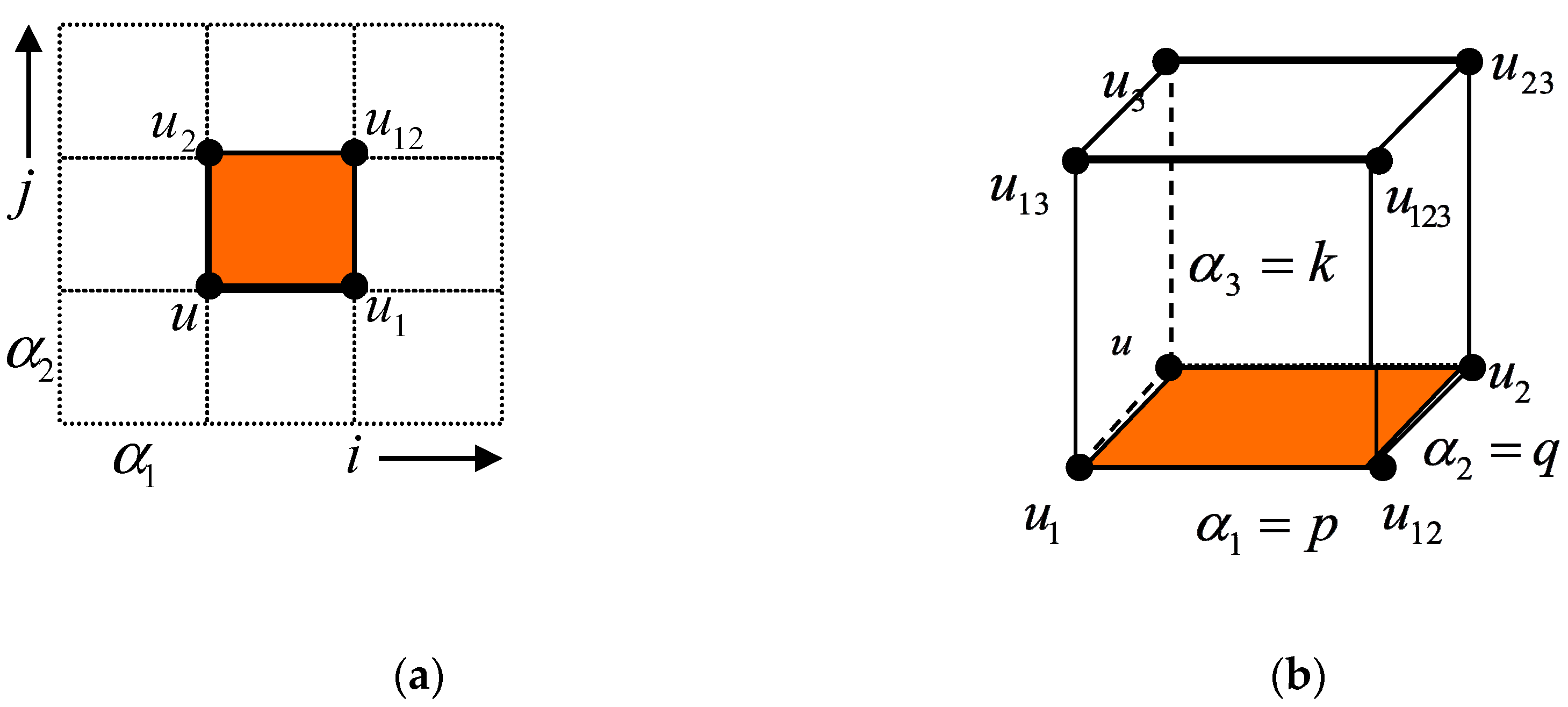
The partial discrete mKdV equation (P∆E mKdV) can be studied through the quadrilateral equation. The quadrilateral equation is used to study the dependent variables in discrete integrated systems via a two-dimensional regular lattice quadratic approach. The method uses a four-sided planar graph (planar quadgraph) that represents the cell decomposition of a surface (see Figure 1a). As shown in Figure 1b, a geometric shape constructed with quadrilaterals is known as a simple cube. A quadrilateral equation is said to have CAC properties if it has the properties of a tetrahedron.
Suppose that a point in a cell is referred to as . Meanwhile, suppose the other three points are and . A simple quadrilateral (orange block in Figure 1) represents an equation that is expressed as
In Equation (1), is affine-linear for all arguments. Thus, for a quadrilateral, as in Figure 1a, Equation (1) is equivalent to
or
where B is a matrix depending on an arbitrary parameter .
In [23], the mathematicians Adler, Bobenko, and Suris (ABS) classified all quadrilateral equations as having CAC properties (tetrahedron properties). For a simple cube, these properties mean that variable depends only on , , and . One of the quadrilateral equations classified as having CAC properties by ABS classification is the P∆E mKdV. On the other hand, the P∆E sine-Gordon is not classified as having CAC properties.
Consider the standard P∆E mKdV equation defined as in [24]:
for the fields defined at the sites of a two-dimensional lattice . In Equation (3), the subscripts denote the values of the independent variable, is the dependent variable, and and are arbitrary constants.
Suppose and . Then, Equation (3) can be written as follows:
Let and . Then, Equation (3) can be expressed with a quadrilateral equation—i.e.,
According to the cube in Figure 1b, several quadrilateral equations can be derived in terms of the down side , left side , back side , top side , right side , and front side . Substituting these quadrilateral equations into Equation (5) and solving for the variable , we arrive at the same quadrilateral equation for the right-top-back side lattices—i.e.,
In Equation (6), the variable depends on , , and only, which means that the P∆E mKdV has CAC properties.
2.2. Traveling Wave Solution for P∆E mKdV (O∆E mKdV)
In [13,25], a four-parameter family of mappings derived from the generalized P∆E mKdV in Equation (4) was studied. Note that a system of ordinary difference equations, O∆E mKdV, can be derived from Equation (4) via the restriction of traveling wave solution with
where and are relatively prime integers (see [26,27] for other applications). Substituting Equation (7) into Equation (4), the following discrete mapping can be obtained:
The map in Equation (8) represents an infinite hierarchy of mappings labeled with and . For fixed and , Equation (8) is a mapping . In [24], for and , the map in Equation (8) has been found to possess several properties—for example, the (anti)measure-preserving property.
Consider the discrete mapping in Equation (8). Let and . This gives the following relation:
The discrete Equation (9) can be written as follows:
where the prime denotes the upshift.
If and , then Equation (10) can be written as
where
Let us assume that is not equal to zero. If , , and , then the following 2D map can be derived from Equation (11):
Furthermore, its integral normal form is (see [13] for other integral normal forms):
where . Thus, for all , the solution for Equation (12) lies in a level set of .
The mapping Equation (12) has several properties:
- Integrable: The mapping has an integral Equation (13), . In other words, is evidently a constant of the mapping’s motion (the orbits of all points in the plane lie on the level sets given by where for any orbit is determined from the initial condition, i.e., .
- Measure-preserving: The mapping is measure-preserving, i.e.,where
- Reversible: There is exists a reversing symmetry such that . It’s means that is reversible (). Note that the mapping is an involution, i.e., , and is identity mapping. The reversibility property ensures that then mapping is invertible.
2.3. Construction of a Two-Dimensional Linear Map (Case Study: Sine-Gordon Map)
Consider a partial discrete sine-Gordon equation on a two-dimensional lattice is defined as follows (see [25,26] for the construction of a generalized sine-Gordon map):
where . A travelling wave solution of Equation (14) was obtained by the ansatz equation (Equation (7)). Therefore, from Equation (14) we then obtained
Let us take and choose and ; we then have the following equation
Equation (16) is equivalent to the mapping
According to Equation (17), we denote by the sequence in , which is defined as . Therefore, a general mapping of the plane , which assigns a point and an image point , can be written as
where
It is easy to check that the mapping (18) has such integrals as follows.
For all , the solution of Equation (16) is on a level set of .
Let us fix λ = 1 to obtain a special case of Equation (18)—namely,
It is easy to check that the mapping in Equation (20) has the integral:
The mapping in Equation (20) has several properties:
- The mapping has an integral equation (Equation (21)).
- is measure-preserving—i.e.,where
- There is a reversing symmetry such that (small circle denoting the symbol for composition). This means that is reversible ().
Note that one of the fixed points on the map is (1,1) [13,26]. Thus, a linear map can be constructed based on the map form in Equation (20) at a closed fixed point (1,1) for which the Jacobian matrix A is written as follows:
From Equation (20) and Equation (22), for , we have the following linear map:
The map described in Equation (23) and Equation (24) can be used for a cryptographic algorithm for a digital image. The maps will be used to change the pixel position of an image without eliminating any information from the image. Note that, due to the reversible map, for the decryption process, we can use the inverse of Equation (24) and the preimage of Equation (23).
2.4. Encryption Scheme for Image Cryptography Based on a Mapping: A Case Study Involving ACM and a 2D Linear Sine-Gordon Map
After developing a mathematical tool, an experiment can be carried out to see how different encryption results will differ using the previous sections mappings. In our experiments, an original image was selected by the authors.
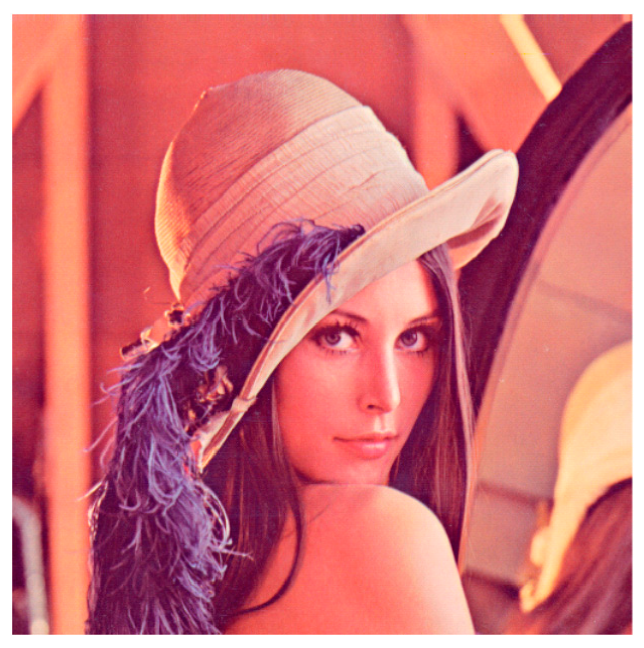
Let us consider Lena plain image in Figure 2. Assume that this image is a private image that will be hidden.
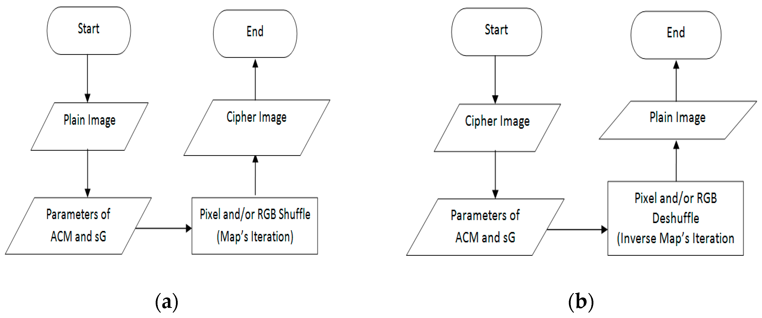
An encryption–decryption scheme for this digital image based on the mappings of (23) and (24) can be constructed as a flow chart in Figure 3.
Based on the encryption algorithm (Figure 3a), the plain image in Figure 2 can be hidden by the following Algorithm 1:
| Algorithm 1: encryption algorithm |
| Input: |
| I: PlainImage (* Figure 2 *); |
| Procedure 2DPlanarMap (: real, numits, dimimage: integer): real; |
| (* numits = number of iterations, |
| and are the entry of matrix coefficient described in Equation (24) *); |
| Begin |
| For i = 1 to numits do |
| For j = 1 to dimimage do |
| Begin |
| ; |
| (* is the map described in Equation (24) and |
| *) |
| End {for j) |
| End {for i}; |
| End{2DPlanarMap } |
| Procedure Image_Transformation (2DPlanarMap:real, I: image): image; |
| Begin |
| Image_Transformation (I, 2DPlanarMap); |
| End{Image_Transformation } |
| {Main Program} |
| Begin |
| Read(I); |
| dimimage Imagedimension(I); |
| Read (, numits); |
| cipherby2DPlanarMap Image_Transformation; |
| Write (cipherby2DPlanarMap); |
| End{Main} |
| Output: |
| chiperby2DPlanarMap: Cipher Image {Figures 4 and 8} |
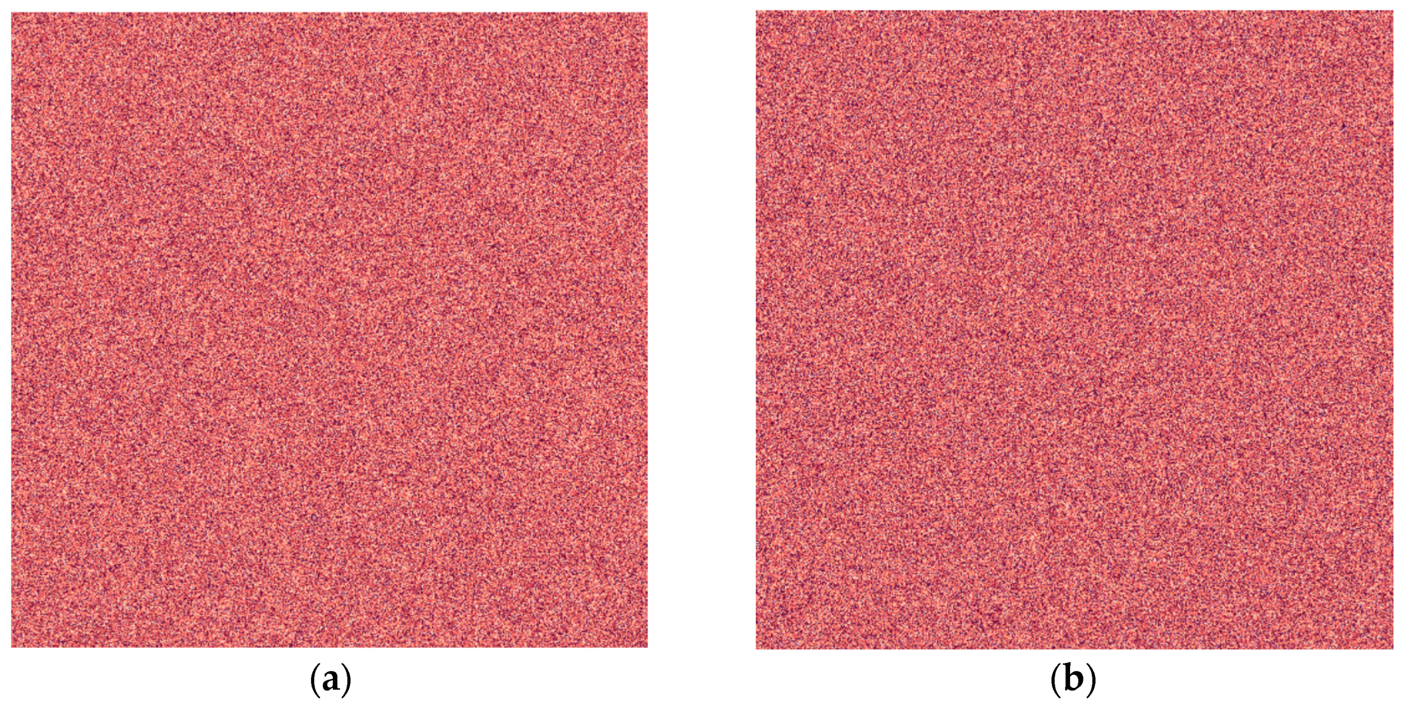
This encryption algorithm for hiding the plain image in Figure 2 in a cipher image is shown in Figures 4 and 8. In Figure 4, the cipher images are the diagrams of the results of the randomization of the original image pixels using a 2D ACM linear map from Equation (24) (Figure 4a) and the 2D sine-Gordon linear map from Equation (23) (Figure 4b). The key parameter values that must be kept secret are µ, p, q, and number of iterations of the map (N). The decryption process requires the same key parameters to retrieve the plain image. To obtain the cipher images based on 2D ACM, we used Equation (24) for and Equation (23) for , respectively.
Note that the cipher images look similar, although they are actually different. To see these differences, pixel data correlations and covariances can be calculated (see Table 1).
3. Results and Discussion
3.1. Dynamics and Bifurcation of the Two-Dimensional mKdV Nonlinear Map
In [26], the dynamics and the bifurcations of the 2D sine-Gordon map in (Equation (20)) were studied. We observed an interesting local bifurcation of critical point in the system—namely, the period doubling bifurcation, where two period–2 points were created from a critical point. For the mapping of all values of , we have four critical points: , , , and . When varies from positive to negative, these critical points change from a saddle type to an elliptic type. Then, we focused on dynamics and bifurcations of the 2-dimensional mKdV map.
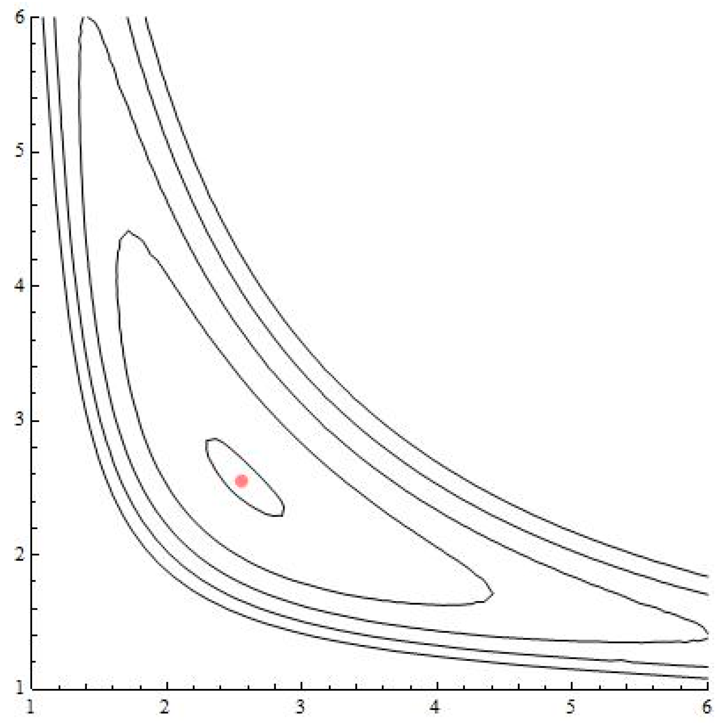
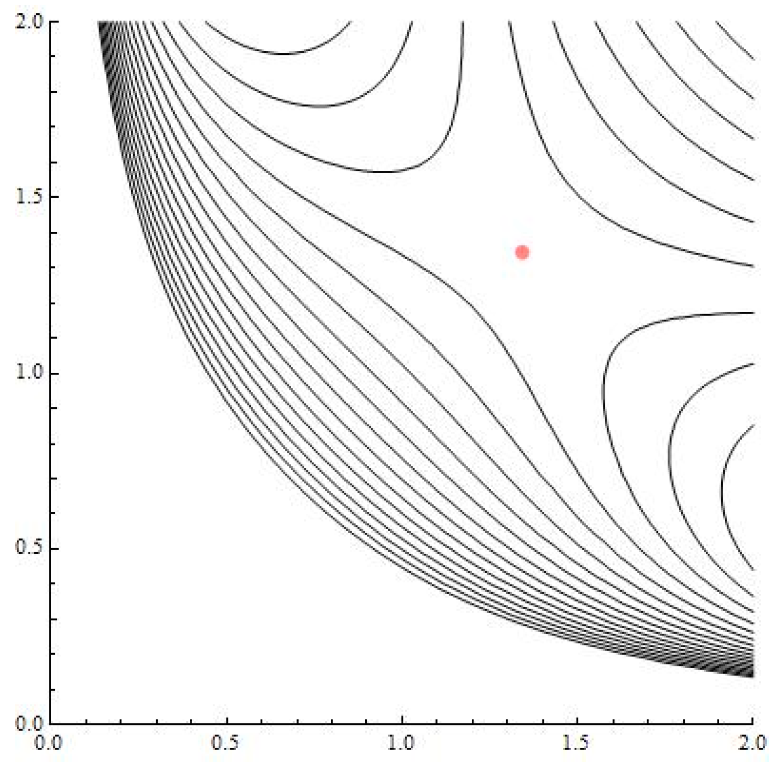
Consider the two-dimensional mKdV map in Equation (12). The dynamics of mapping is contained in the level sets of . In Figure 5, Figure 6 and Figure 7, we have plotted a few of the level sets the function for various values of parameter . We obtained a nonlocal bifurcation involving collision of homoclinic and heteroclinic connections between saddle type critical points (see Figure 6). Additionally, we obtained a change in stability of a critical point from a saddle type into an elliptic type.
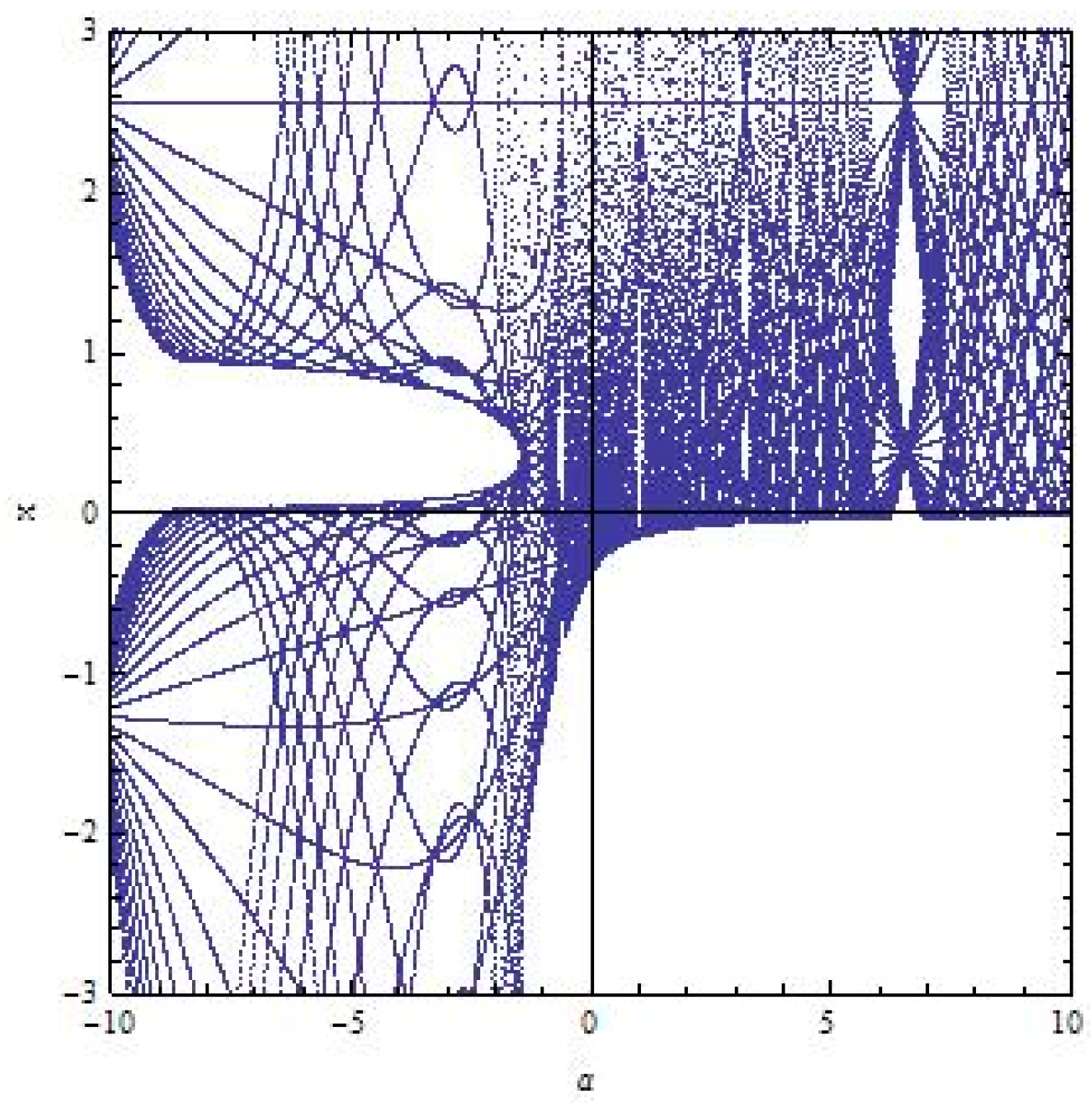
Bifurcations. The word “bifurcation” refers to a sudden qualitative change in the nature of solutions that occurs as the parameter is varied. The bifurcation diagram shows many sudden qualitative changes in the attractor as well as in the periodic orbits [29].
Considering the level set diagrams in Figure 5, Figure 6 and Figure 7, when varies, the critical points of change from an elliptic type to a saddle type. A known mechanism in the literature, for integrable systems, is through a Saddle-Center bifurcation, where one saddle point becomes degenerate, and breaks into three critical points: two saddles and one elliptic (or also known as center) point [26]. In the case of , the bifurcation diagram with respect to varying of is shown in Figure 8. Note that the blue dots that spread out represent the chaotic region.
The Maximum Lyapunov Exponent: The chaotic behavior of a dynamical system is defined by its sensitiveness to initial conditions and unpredictability. The Lyapunov exponent (LE) is a quantitative measurement to determine the dynamical system’s chaotic behavior [30]. LE measures the degree of divergence between any two nearby trajectories of a dynamical system, stretching an orbit. The positive value of maximum LE shows exponential stretching of an orbit. Every chaotic system has at least one positive Lyapunov exponent to achieve chaotic behavior.
A multidimensional chaotic map with more than one LE, and if all the LEs are positive, then the dynamical systems possess hyperchaotic behavior. The hyperchaotic behavior is good for image encryption and it is very difficult for the attacker to predict the secret key [31]. For two-dimensional map , in Equation (12) for example, we can calculate the maximum LE, at the point by using the following formula [29]:
where
- ,
- ,
- .
Now, we can use to acquire the maximum LE for 2D nonlinear mKdV map in Equation (12). For and the fixed point , we have
Substituting , we get and . Finally, we have the maximum LE number is . Thus, the orbit of the mapping in Equation (12) is exponential stretching.
3.2. Two-Dimensional Linear Map Derived from a Nonlinear O∆E mKdV Map
An essential element in the construction of the linear system in Equation (12) is a fixed point. A fixed point can be obtained by finding the critical point of the integral function. The critical points of the integral in Equation (12) are the solutions of
and
After taking the difference between the two equations, we have a line . By substituting these solutions into one of the equations, we have the following critical points that depend on :
where , , , , , , where .
Let be an interval in (finite). Assume that . For , we then have some fixed point values, as seen in Table 2.
To construct a linear map derived from the map in Equation (12) around a fixed point , we can use the values of in Table 2. Thus, a linear map can be constructed based on the Jacobian matrix as follows:
From Equation (12) and Equation (29), for , we have the following linear map:
For example, at and the point , we have a linear map—namely,
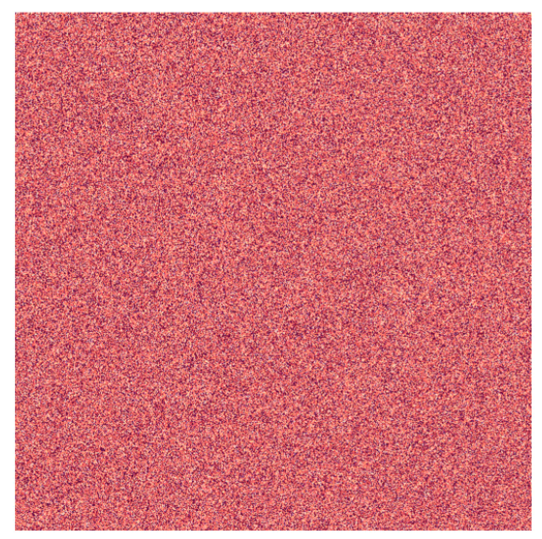
Once more, based on the encryption algorithm in Figure 3a, we used 2D linear mKdV map in Equation (31) to hide the plain image in Figure 2. Applying the linear map in Equation (31), we obtained the cipher image shown in Figure 9.
Note that we used the values of , fixed point , and number of iterations N = 110 to obtain the cipher image shown in Figure 9. They are key values that must be kept secret.
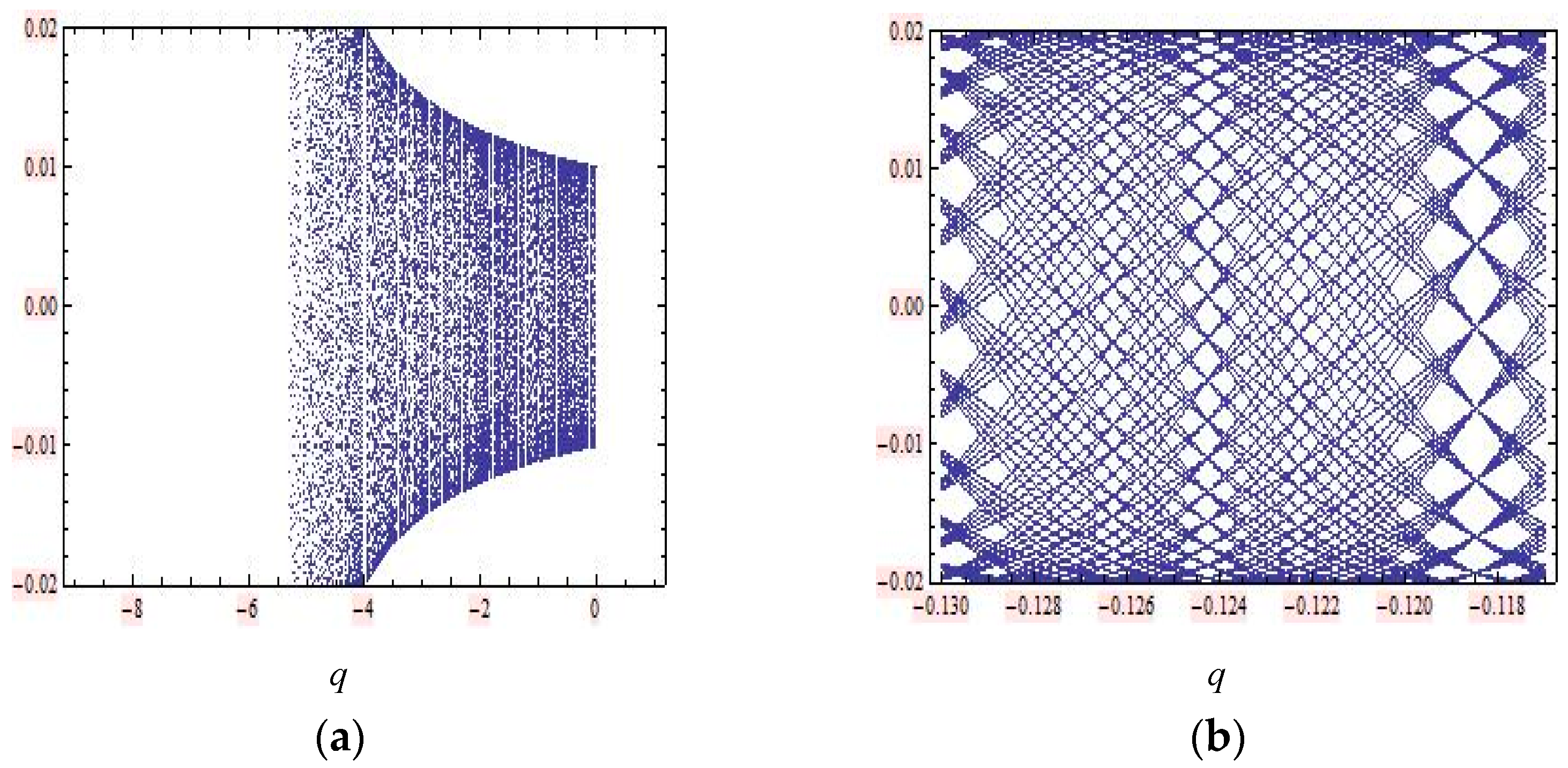
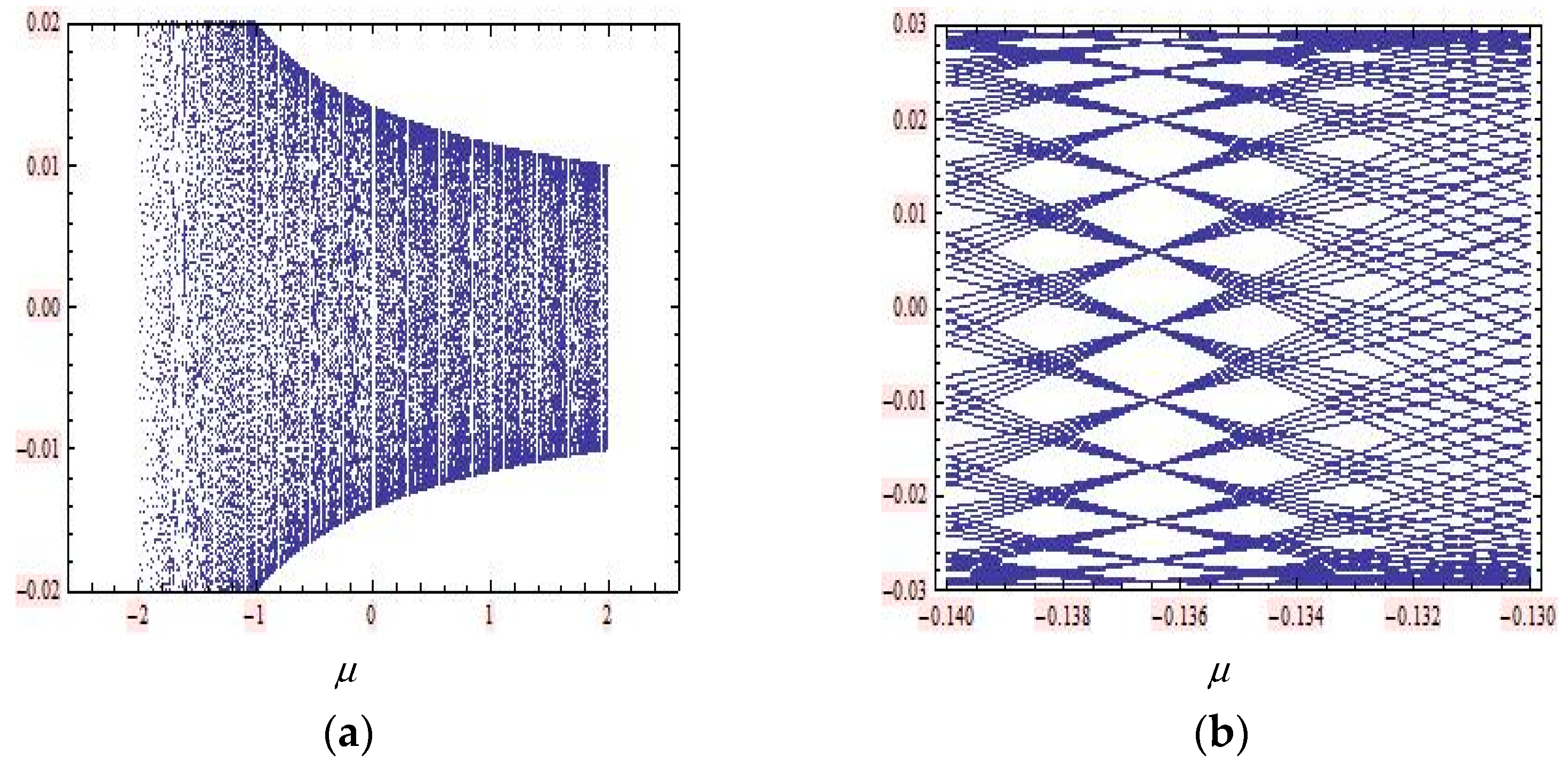
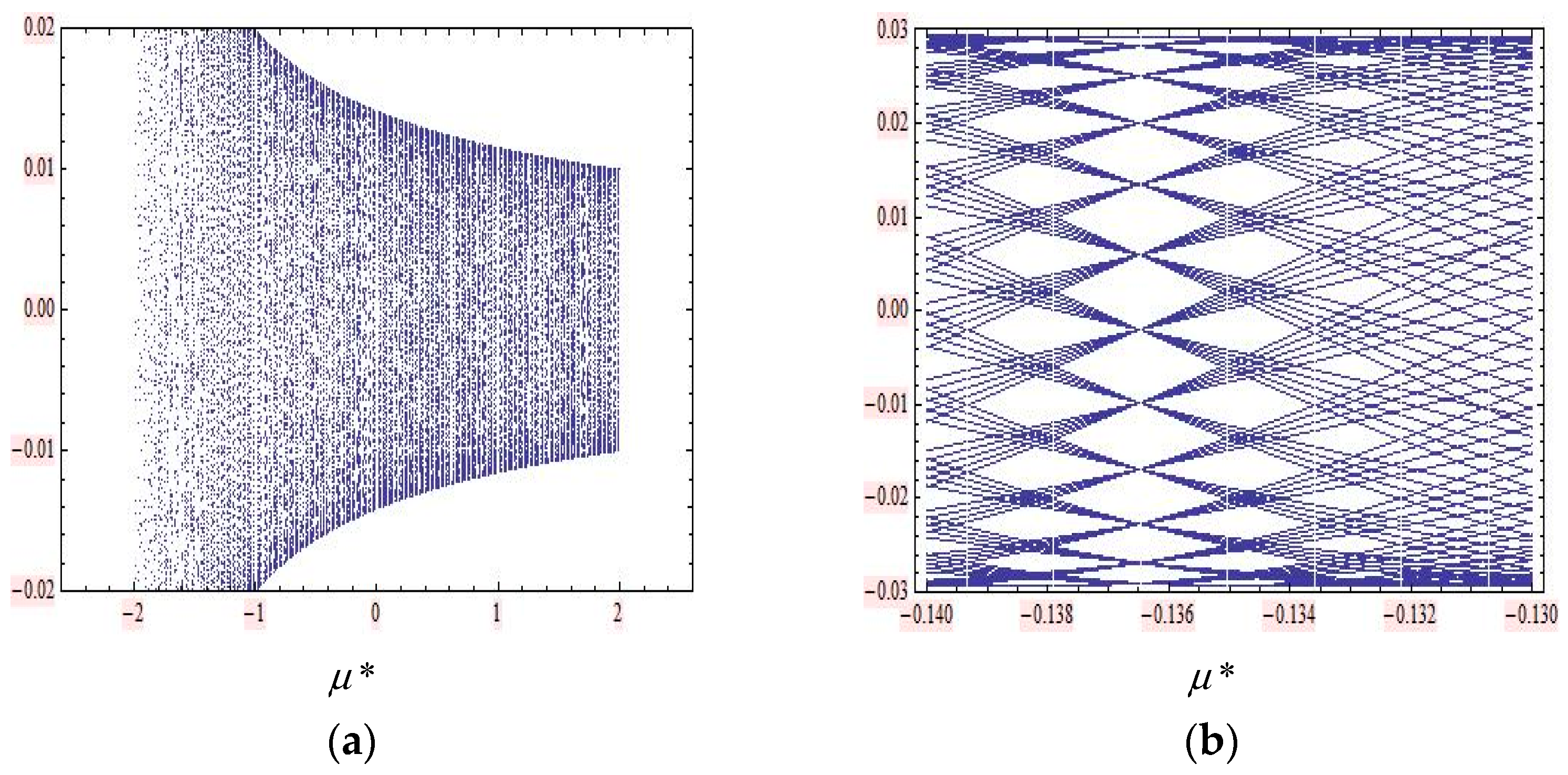
We have already seen that in Figure 6, Figure 7 and Figure 8, different values of the parameter may yield qualitatively different solutions. We are especially interested in the changing nature of solutions as the parameter is varied. To investigate such changes, we shall use the bifurcation diagram plot for all linear maps discussed in this article. Next, we will show the bifurcation diagrams for the 2D linear ACM in Equation (24), sine-Gordon in Equation (23), and mKdV map in Equation (31). These maps have as a fixed point. Using Mathematica, the bifurcation diagrams around can be obtained and are shown in Figure 10, Figure 11 and Figure 12.
For the bifurcation diagram in Figure 10, we fixed p = 0.75 and use a parameter q in bifurcation plots. First, we started with the bifurcation diagram where , with 300 steps; 200 is the number of the first iteration shown, 150 is the maximum number of iterations, and (0.01, 0.01) is the starting point of the iteration. The range in the vertical axis is set to (−0.02, −0.02). Zooming in, we acquired an interesting “net pattern”. The bifurcation values for the periodic solutions of periods 19 can be located precisely on this plot with around . In the same procedure, to produce the bifurcation diagrams in Figure 11, we used the parameter values of in bifurcation plots. Zooming in, we acquired an interesting “net pattern”. The bifurcation values for the periodic solutions of periods 21 can be located precisely on this plot with around . As for the 2D sine-Gordon map, to produce the bifurcation diagrams for the 2D mKdV map, as shown in Figure 12, we fixed a parameter in bifurcation plots. This gave us the same bifurcation diagrams as with the 2D sine-Gordon map.
Consider the LE formula in Section 3.1. We can use the formula to obtain the LEs for the 2D linear ACM map, sine-Gordon map, and mKdV map and also the Lyapunov number that defined as the exponent of the LE, , as shown in Table 3.
Based on Table 3, the 2D linear sine-Gordon map and the 2D linear mKdV map are chaotic systems.
3.3. Histogram, Covariance, and Correlation Computations Based on the Weighted Data in the Image Pixels
When considering cryptographic image data processing, there are two important tools used to analyze image processing—i.e., the gradient filter and the gradient orientation filter. The gradient filter provides an image corresponding to the image gradient’s magnitude and is computed using the discrete derivatives of a Gaussian of the pixel radius. Meanwhile, the gradient orientation filter provides an image corresponding to the local orientation that is parallel to the image gradient and is computed using the discrete derivatives of a Gaussian of the pixel radius, thus returning values between and [32].
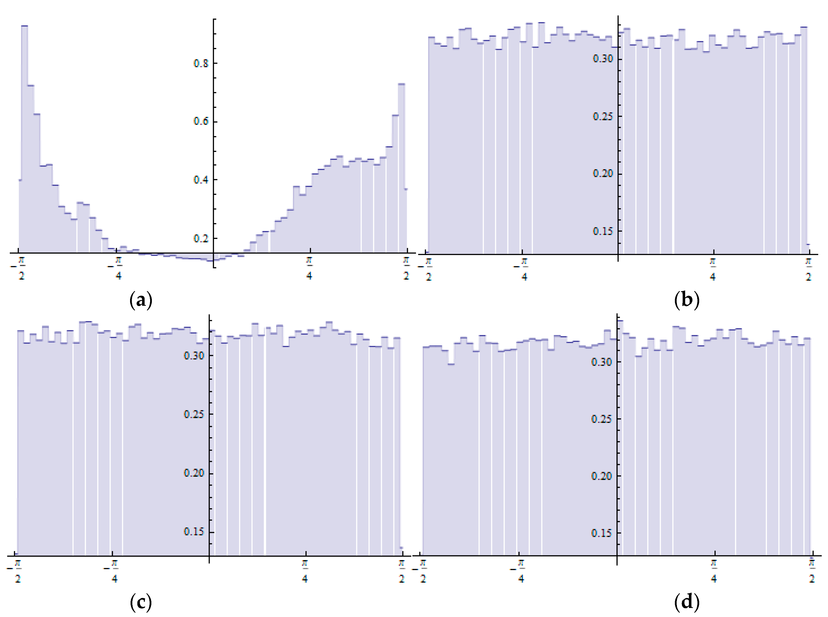
The important analyses for image cryptography via encryption algorithms are the histogram, covariance, and correlation analyses. Histogram analysis is conducted to determine the pixel distribution. The distribution of an image’s pixel values prior to encryption is usually concentrated on the pixels’ highest space value. Therefore, the best encryption spreads the pixel values out over the pixel space. Another tool, the adjacent pixel correlation, was used to test the correlations between pairs of adjacent pixels.
Mathematica was used to produce the histogram distributions for the ACM encryption in Equation (24), 2D linear map in Equation (23), and 2D linear map in Equation (31). Four histogram distributions of the weighted data for the images shown in Figure 2, Figure 4 and Figure 9 are shown in Figure 13. There are clear differences between the histograms for the plain image and those for the cipher images.
Generally, the histograms generated by the cipher images have flat distributions (uniform). In contrast, the histogram generated by the plain image focuses on some space pixel values. The covariances and correlations for the image data for N = 110 iterations are shown in Table 4.
4. Conclusions
A 2D linear map derived from an O∆E mKdV equation was constructed. The 2D mKdV linear map can be used for the cryptographic encoding of an image. Based on the implementation of the encoding algorithm, a linear map derived from generalized sine-Gordon mapping can be used to secure a digital image. We compared three linear mappings—namely, the 2D Arnold’s cat map, 2D sine-Gordon linear map, and 2D mKdV linear map—in terms of their abilities to conceal an image. The comparison showed that the 2D mKdV linear map provided a very low correlation value compared to the other two mappings, which means that the 2D mKdV linear map provides a higher level of encryption. Nevertheless, we cannot conclude that the 2D mKdV linear map provides the best results under all conditions. However, this mapping’s decryption results can be tested using the concept of dilation and erosion operation, which is a crucial image processing algorithm. One method used in dilation and erosion operations is the quantum method (see [33] for details). Other than that, in the process of restoring the original image (decryption), we recommend that our proposed mappings be tested for resisting a certain degree of source noise pollution and effectively recover the original signal (see [9,34] for details). Further investigation is necessary.
Author Contributions
Conceptualization, L.Z. and A.A.; methodology, L.Z. and E.Y.; software, L.Z. and E.Y.; validation, L.Z., A.A. and E.Y.; formal analysis, L.Z.; investigation, L.Z. and E.Y.; resources, L.Z. and A.A.; data curation, L.Z.; writing—original draft preparation, L.Z.; writing—review and editing, L.Z. and A.A.; visualization, L.Z. and E.Y.; supervision, L.Z.; project administration, L.Z.; funding acquisition, A.A. All authors have read and agreed to the published version of the manuscript.
Funding
This research was funded by Directorate of Research and Community Services at Kemendikbud RI grant number 044/SP2H/LT/DRPM/2020 and the APC was funded by First Author.
Institutional Review Board Statement
Not applicable.
Informed Consent Statement
Not applicable.
Acknowledgments
The authors would like to thank the Directorate of Research and Community Services at Kemendikbud RI for funding this research through Research Grant 044/SP2H/LT/DRPM/2020 and the Head of the Institute of Research and Community Services of Lampung University, who supported this research.
Conflicts of Interest
The authors confirm that they have no conflict of interest to declare.
References
- Elgamal, T. A public key cryptosystem and a signature scheme based on discrete logarithms. Lect. Notes Comput. Sci. (Incl. Subser. Lect. Notes Artif. Intell. Lect. Notes Bioinform.) 1985, 31, 10–18. [Google Scholar]
- Munir, R. Algoritma enkripsi selektif citra digital dalam Ranah frekuensi berbasis permutasi chaos (digital image selective encryption algorithm in frequency domain based on chaos permutation). J. Rekayasa Elektr. 2015, 10, 66–72. [Google Scholar]
- Hidayat, A.D.; Afrianto, I. Sistem kriptografi citra digital pada jaringan intranet menggunakan metode kombinasi chaos map dan teknik selektif (digital image cryptography system on intranet network using combination method of chaos map and selective techniques). J. Ultim. 2017, 9, 59–66. [Google Scholar] [CrossRef] [Green Version]
- Ronsen, P.; Halim, A.; Syahputra, I. Enkripsi citra digital menggunakan Arnold’s cat map dan nonlinear chaotic algorithm (digital image encryption using Arnold’s cat map and nonlinear chaotic algorithm). JSM STMIK Mikroskil 2014, 15, 61–71. [Google Scholar]
- Soleymani, A.; Nordin, J.; Sundararajan, E. A chaotic cryptosystem for images based on Henon and Arnold cat map. Sci. World J. 2014, 2014, 1–21. [Google Scholar] [CrossRef] [Green Version]
- Abbas, N.A. Image encryption based on independent component analysis and Arnold’s cat map. Egypt. Inform. J. 2016, 17, 139–146. [Google Scholar] [CrossRef] [Green Version]
- Revanna, C.R.; Keshavamurthy, C. A secure document image encryption using mixed chaotic system. Int. J. Appl. Eng. Res. 2017, 12, 8854–8865. [Google Scholar]
- Abaas, S.A.; Shibeeb, A.K. A new approach for video encryption based on modified AES algorithm. IOSR J. Comput. Eng. 2015, 17, 44–51. [Google Scholar]
- IEEE-Indonesia; Munir, R. Robustness Analysis of Selective Image Encryption Algorithm Based on Arnold Cat Map Permutation. In Proceedings of the 3rd Makassar International Conference on Electrical Engineering and Informatics (MICEEI), Makassar, Indonesia, 28 November–1 December 2012; pp. 1–5. [Google Scholar]
- Fu, C.; Chen, Z.; Zhao, W.; Jiang, H. A New Fast Color Image Encryption Scheme Using Chen Chaotic System. In Proceedings of the International Conference on Software Engineering, Artificial Intelligence, Kazanawa, Japan, 26–28 June 2017; Networking and Parallel/Distributed Computing (SNPD 2017): Los Alamitors, CA, USA, 2017; pp. 121–126. [Google Scholar]
- Abbadi, N.K.E.; Yahya, E.; Aladilee, A. Digital RGB Image Encryption Based on 2D Cat Map and Shadow Numbers. In Proceedings of the Annual Conference on New Trends in Information & Communications Technology Applications (NTICT 2017), Baghdad, Iraq, 7–9 March 2017; IEEE: Pistacaway, NJ, USA, 2017; pp. 162–167. [Google Scholar]
- Tan, Y.-F.; Guo, X.; Tan, W.-N. Reversible data hiding using reference points coding. In Proceedings of the 2017 IEEE 2nd Information Technology, Networking, Electronic and Automation Control Conference (ITNEC), Chengdu, China, 12–15 December 2017; pp. 55–59. [Google Scholar]
- Zakaria, L.; Notiragayu, N.; Nuryaman, A.; Suharsono, S. The integral normal form of a three-dimensional traveling wave solution mapping derived from generalized ∆∆-mKdV equation. Adv. Differ. Equ. Control Process. 2018, 19, 37–48. [Google Scholar] [CrossRef] [Green Version]
- Yuliani, E.; Zakaria, L. Asmiati A Two-Dimensional Map Derived From An Ordinary Difference Equation of mKdV and Its Properties. J. Phys. Conf. Ser. 2021, 1751, 012010. [Google Scholar] [CrossRef]
- Notiragayu, N.; Zakaria, L. The Implementation of Digital Text Coding Algorithm Through A Three Dimensional Mapping Derived from Generalized ΔΔ-mKdV Equation Using Mathematica. In Proceedings of the International Conference on Applied Sciences Mathematics and Informatics (ICASMI 2018), Bandar Lampung, Indonesia, 9–11 August 2018; Institute of Physics-UK: London, UK, 2019; Volume 1338, p. 7. [Google Scholar]
- Schief, W.K. Lattice geometry of the discrete darboux, KP, BKP, and CKP equations. Menelaus’ and Carnot’s theorems. J. Non-Linear Math. Phys. 2003, 10, 194–208. [Google Scholar] [CrossRef]
- Susanto, H.; Karjanto, N.; Zulkarnain; Nusantara, T.; Widjanarko, T. Soliton and breather splitting on star graphs from tricrystal josephson junctions. Symmetry 2019, 11, 271. [Google Scholar] [CrossRef] [Green Version]
- Ablowitz, M.J.; Ladik, J.F. Nonlinear differential-difference equations and Fourier analysis. J. Math. Phys. 1976, 17, 1011–1018. [Google Scholar] [CrossRef]
- Islam, S.; Khan, K.; Akbar, M.A. An analytical method for finding exact solutions of modified Korteweg–de Vries equation. Results Phys. 2015, 5, 131–135. [Google Scholar] [CrossRef] [Green Version]
- Das, A. Integrable Models (Work Scientific Lecture Notes in Physics); Work Scientific Publishing Co. Pte. Ltd.: Singapore, 1989; p. 30. [Google Scholar]
- Kou, X.; Zhang, D.J.; Shi, Y.; Zhao, S.L. Generating solutions to discrete Sine-Gordon equation from modified Backlund transformation. Commun. Theor. Phys. 2011, 55, 545–550. [Google Scholar] [CrossRef]
- der Kamp, P.H.V. Initial value problems for lattice equations. J. Phys. A Math. Theor. 2009, 42, 404–419. [Google Scholar] [CrossRef]
- Adler, V.; Bobenko, A.; Suris, Y. Classification of integrable equations on quad-graphs. The consistency approach. Commun. Math. Phys. 2003, 233, 513–543. [Google Scholar] [CrossRef] [Green Version]
- Hietarinta, J. Searching for CAC-maps. J. Nonlinear Math. Phys. 2005, 12, 223–230. [Google Scholar] [CrossRef]
- Zakaria, L.; Tuwankotta, J.M. Dynamics of A Re-Parametrization of A 2-Dimensional mapping derived from double discrete Sine-Gordon mapping. Int. J. Math. Eng. Manag. Sci. 2020, 5, 363–377. [Google Scholar] [CrossRef]
- Zakaria, L.; Tuwankotta, J.M. Dynamics and bifurcations in a two-dimensional map derived from a generalized\delta\delta-sine-gordon equation. Far East J. Dyn. Syst. 2016, 28, 165–194. [Google Scholar] [CrossRef]
- Quispel, G.; Capel, H.; Papageorgiou, V.; Nijhoff, F. Integrable mappings derived from soliton equations. Phys. A Stat. Mech. Its Appl. 1991, 173, 243–266. [Google Scholar] [CrossRef]
- Implementing Arnold’s Cat Map. Available online: https://mathematica.stackexchange.com/questions/164070/implementing-arnolds-cat-map (accessed on 22 July 2019).
- Kulenovic, M.R.S.; Merino, O. Discrete Dynamical Systems and Difference Equations with Mathematica; Chapman and Hall/CRC: Boca Raton, FL, USA, 2002. [Google Scholar]
- Mondal, B.; Behera, P.K.; Gangopadhyay, S. A secure image encryption scheme based on a novel 2D sine–cosine cross-chaotic (SC3) map. J. Real-Time Image Process. 2021, 18, 1–18. [Google Scholar] [CrossRef]
- Ali, M.; Saha, L. Local Lyapunov Exponents and characteristics of fixed/periodic points embedded within a chaotic attractor. J. Zhejiang Univ. A 2005, 6A, 296–304. [Google Scholar] [CrossRef]
- Mathematica Online: www. wolfram.com; Wolfram Research Inc.: Champaign, IL, USA, 2002.
- Ma, S.-Y.; Khalil, A.; Hajjdiab, H.; Eleuch, H. Quantum dilation and erosion. Appl. Sci. 2020, 10, 4040. [Google Scholar] [CrossRef]
- Yu, J.; Xie, Y.; Guo, S.; Zhou, Y.; Wang, E. Parallel encryzption of noisy images based on sequence generator and chaotic measurement matrix. Complexity 2020, 2020, 1–18. [Google Scholar] [CrossRef]
Figure 1.
Simple quadrilateral (a) and simple cube (b).

Figure 2.
An example of an original (plain) image.

Figure 3.
A flow chart for an encryption (a) and decryption (b) algorithm.

Figure 4.
Cipher images after using Arnold’s Cat Map (ACM) (a) and sine-Gordon (b) map obtained from encrypting the original image in Figure 2 with Equation (24) and Equation (23).
Figure 4.
Cipher images after using Arnold’s Cat Map (ACM) (a) and sine-Gordon (b) map obtained from encrypting the original image in Figure 2 with Equation (24) and Equation (23).

Figure 5.
The level set of for . The fixed point is stable.

Figure 6.
The level set of for . The fixed point is stable.

Figure 7.
The level set of for . The fixed point is unstable.

Figure 8.
A bifurcation diagram of for and .

Figure 9.
The cipher image obtained after using the 2D linear map in Equation (31) on the original image in Figure 2.
Figure 9.
The cipher image obtained after using the 2D linear map in Equation (31) on the original image in Figure 2.

Figure 10.
Two bifurcation diagrams and a Lyapunov exponent (LE) curve of the 2D ACM linear map in Equation (24) around fixed point . (a) Bifurcation diagram for plotting . (b) Bifurcation diagram for zooming around .
Figure 10.
Two bifurcation diagrams and a Lyapunov exponent (LE) curve of the 2D ACM linear map in Equation (24) around fixed point . (a) Bifurcation diagram for plotting . (b) Bifurcation diagram for zooming around .

Figure 11.
Two bifurcation diagrams of the 2D sine-Gordon linear map in Equation (23) around fixed point . (a) Bifurcation diagram for plotting . (b) Bifurcation diagram for zooming around .
Figure 11.
Two bifurcation diagrams of the 2D sine-Gordon linear map in Equation (23) around fixed point . (a) Bifurcation diagram for plotting . (b) Bifurcation diagram for zooming around .

Figure 12.
Two bifurcation diagrams of the 2D mKdV linear map in Equation (22) around fixed point . (a) Bifurcation diagram for plotting . (b) Bifurcation diagram for blowing up around .
Figure 12.
Two bifurcation diagrams of the 2D mKdV linear map in Equation (22) around fixed point . (a) Bifurcation diagram for plotting . (b) Bifurcation diagram for blowing up around .

Figure 13.
Histogram distributions based on weighted data: (a) Distribution of the plain image (before encryption). (b) Distribution of the cipher image after encryption with ACM in Equation (24). (c) Distribution of the cipher image after encryption with the 2D linear map in Equation (23). (d) Distribution of the cipher image after encryption with the 2D linear map in Equation (31).


Table 1.
The computation of the covariances and correlations of the image data based on the weighted data (gradient orientation filter, gradient filter) for the images.
Table 1.
The computation of the covariances and correlations of the image data based on the weighted data (gradient orientation filter, gradient filter) for the images.
| Covariance | Correlation | |
|---|---|---|
| Plain Image (Figure 2) | 0.000919690 | 0.024302828 |
| Cipher Image Generated by Equation (24) (Figure 4a) | −0.000001413 | −0.000078930 |
| Cipher Image Generated by Equation (23) (Figure 4b) | 0.000005278 | 0.000295260 |
Table 2.
The relationship between the parameter values and fixed points for three values of α.
| No. | α | Fix Point | Fixed Point Positions |
|---|---|---|---|
| 1. | |||
| 2. | |||
| 3. |
Table 3.
The LE number and LN number for the 2D linear ACM map (Equation (24)), the 2D linear sine-Gordon map (Equation (23)), and the 2D linear mKdV map (Equation (31)) closed fixed points
Table 3.
The LE number and LN number for the 2D linear ACM map (Equation (24)), the 2D linear sine-Gordon map (Equation (23)), and the 2D linear mKdV map (Equation (31)) closed fixed points
| No. | 2D Linear Map | LE: | LN: | |
|---|---|---|---|---|
| 1. | ACM | (0.001, 0.001) | 0.9533117189 | 2.59428699560 |
| 2. | sine-Gordon | (0.001, 0.001) | 6.6821101678 | 798.001253131 |
| 3. | mKdV | (0.001, 0.001) | 0.7638455683 | 2.14651493883 |
Table 4.
The covariances and correlations of the image data based on the weighted data (gradient orientation filter, gradient filter) of the image for N = 110 iterations.
Table 4.
The covariances and correlations of the image data based on the weighted data (gradient orientation filter, gradient filter) of the image for N = 110 iterations.
| Covariance | Correlation | |
|---|---|---|
| Plain Image | 0.001048070 | 0.01704610 |
| Cipher Image Generated by Equation (24) | 0.000202934 | 0.00928261 |
| Cipher Image Generated by Equation (23) | 0.000042265 | 0.00187458 |
| Cipher Image Generated by Equation (31) | −0.00000098 | −0.00041965 |
Publisher’s Note: MDPI stays neutral with regard to jurisdictional claims in published maps and institutional affiliations. |
© 2021 by the authors. Licensee MDPI, Basel, Switzerland. This article is an open access article distributed under the terms and conditions of the Creative Commons Attribution (CC BY) license (https://creativecommons.org/licenses/by/4.0/).
Share and Cite
MDPI and ACS Style
Zakaria, L.; Yuliani, E.; Asmiati, A. A Two-Dimensional mKdV Linear Map and Its Application in Digital Image Cryptography. Algorithms 2021, 14, 124. https://0-doi-org.brum.beds.ac.uk/10.3390/a14040124
AMA Style
Zakaria L, Yuliani E, Asmiati A. A Two-Dimensional mKdV Linear Map and Its Application in Digital Image Cryptography. Algorithms. 2021; 14(4):124. https://0-doi-org.brum.beds.ac.uk/10.3390/a14040124
Chicago/Turabian StyleZakaria, La, Endah Yuliani, and Asmiati Asmiati. 2021. "A Two-Dimensional mKdV Linear Map and Its Application in Digital Image Cryptography" Algorithms 14, no. 4: 124. https://0-doi-org.brum.beds.ac.uk/10.3390/a14040124
Note that from the first issue of 2016, this journal uses article numbers instead of page numbers. See further details here.