
A Multinomial DGA Classifier for Incipient Fault Detection in Oil-Impregnated Power Transformers


1
African Center of Excellence in Internet of Things, University of Rwanda, Kigali P.O. Box 42 85, Rwanda
2
Department of Computer Science, Egerton University, Egerton P.O. Box 536-20115, Kenya
*
Author to whom correspondence should be addressed.
Algorithms 2021, 14(4), 128; https://0-doi-org.brum.beds.ac.uk/10.3390/a14040128
Submission received: 25 January 2021
/
Revised: 4 March 2021
/
Accepted: 30 March 2021
/
Published: 20 April 2021
(This article belongs to the Special Issue Supervised and Unsupervised Classification Algorithms)
Abstract
:This study investigates the use of machine-learning approaches to interpret Dissolved Gas Analysis (DGA) data to find incipient faults early in oil-impregnated transformers. Transformers are critical pieces of equipment in transmitting and distributing electrical energy. The failure of a single unit disturbs a huge number of consumers and suppresses economic activities in the vicinity. Because of this, it is important that power utility companies accord high priority to condition monitoring of critical assets. The analysis of dissolved gases is a technique popularly used for monitoring the condition of transformers dipped in oil. The interpretation of DGA data is however inconclusive as far as the determination of incipient faults is concerned and depends largely on the expertise of technical personnel. To have a coherent, accurate, and clear interpretation of DGA, this study proposes a novel multinomial classification model christened KosaNet that is based on decision trees. Actual DGA data with 2912 entries was used to compute the performance of KosaNet against other algorithms with multiclass classification ability namely the decision tree, k-NN, Random Forest, Naïve Bayes, and Gradient Boost. Investigative results show that KosaNet demonstrated an improved DGA classification ability particularly when classifying multinomial data.
1. Introduction
The transformer is an indispensable piece of equipment in generating, transmitting, and distributing electricity [1]. They are also expensive and account for massive capital expenditure in the contemporary electrical network. Not only do they require huge fiscal investments but the reliability and dependability of the entire electricity grid depends primarily on their operational stability [2,3,4,5]. It is, therefore, imperative that utility companies give priority to failure prevention and the sustenance of optimal operational status of their electrical network. Maintaining these assets in an optimal and efficient state is a key priority of many electric utilities globally. In fact, a huge portion of the annual budget of these utility companies is allocated to condition monitoring and maintenance of these assets [6,7,8]. Condition monitoring and asset management is therefore a key concern in all electric utility providers. With a typical electrical network deploying transformers in their thousands, condition monitoring easily becomes a labor-intensive and time-consuming exercise.
The basic principle upon which a transformer works is that of mutually induced magnetic flux that links the primary with the secondary windings. When an alternating current flows through the primary windings, it induces a voltage that is greater than or less than that across the secondary windings depending on whether the unit is a stepdown or step-up transformer [1,9]. The frequency of the induced and inducing voltages however remain unchanged. Figure 1 illustrates the basic manner of construction of a transformer.
The transformer comprises of an intricate arrangement of a pair of coils wound on an iron core. To prevent the iron core from acting as a conductor, it is assembled using thin layers of varnish coated steel [10]. During normal operation, an alternating current on the primary windings produces a changing flux within the core. The flux in turn induces an electromotive force (emf) within the core that in turn sets up the circulating currents called Eddy Currents. Eddy currents produces losses, which manifest as heat. The magnitude of this loss can be calculated by Equation (1) [11].
where Pe is the hysteresis loss in Watts, Ke is the stein Metz hysteresis coefficient; t is the material thickness; Bm is the flux; f the rate of magnetic oscillations and V volume of in m3.
As is seen from Equation (1), the heating up of a transformer during operation is anticipated. The concern therefore is how to prevent and manage the excessive build-up of heat to destructive levels. Several techniques have been used to accomplish this. One of these being to immerse the transformer core and winding in mineral oil. Oil not only acts as a coolant but also is itself also an insulating material [12].
Recent studies suggest that many transformers do not live up to their expected lifetime of between 25–35 years [2]. In Kenya for instance, as many as 10–12% of the population of distribution transformers are prematurely retired against an international annually rate of between 1 and 2% in the more industrialized countries [2]. The failure of a single transformer disrupts economic activities for both the consumers and utility company [13]. For continued reliability and availability there must be continuous monitoring and maintenance of the transformer. However, with the huge number of transformers deployed in an electrical network, monitoring, and maintenance is a daunting task that requires massive labor and time. Kenya Power has reported that it owns about 70,000 transformers countrywide deployed at various locations scattered all around the country [14].
Dissolved and free gas analysis is a widely used and highly regarded means of detecting incipient faults in oil-immersed transformers. DGA reliably gauges a transformer’s operational status and is extensively used in routine maintenance [15,16]. It is an investigative process in which oil samples collected from oil-immersed transformers are inspected for fault gases. The concentration, ratio, and type of the gases tell a tale about the internal condition of the transformer. Insulating oil not only performs functions such as cooling the unit and dousing arcs, but more significantly, it dissolves any gases produced as a result of cellulose deterioration or ambient moisture from the environment. A common cause of early failure of transformer units is the deterioration of insulating oil. It is estimated that about 70–80% of the faults in a transformer are incipient in nature which implies that any effort to detect these faults can potentially reduce the manifestation of faults on the grid by a similar margin [15,17].
Classical methods of DGA interpretation include Key Gases, Duval and Nomography [18]. The interpretation of DGA data has for decades relied on these classical approaches. These classical approaches however tend to rely extensively on the experience, judgment, and intuition of a human expert rather than technical formulation. This reliance on a human benefactor has often led to an inconclusive assessment of the severity of the faults or in the extreme case, a misidentification altogether [19]. Numerous studies have been conducted that propose methods by which the severity of incipient power transformers faults can be determined. In [20] for instance, Prasojo et al. studied fuzzy logic to determine faults on power transformers created by using gas levels and gas rates as well as interpreted DGA data. The Duval Pentagon Method (DPM) was assimilated with the Support Vector Machine (SVM) algorithm being the chosen interpretation method. The study resulted in an accuracy score of 97.5%. In [21] a study was conducted which designed a smart fuzzy reinforcement learning-based fault classifier for transformers. DGA data, collected from actual transformers and other credible secondary sources, were used. The results showed that the suggested fuzzy reinforcement learning technique is superior as compared to other contemporary approaches attaining an accuracy score of 99.7%. Fuzzy logic models however tend to perform poorly when subjected to new data. In [22] a multilayer perceptron (MLP) network is discussed with boundaries defined using a fuzzy class. The model is centered on the Duval Pentagon and gas ratio combination. A multilayer perceptron network was trained on actual DGA records with fault conditions specifically marked. The proposed method had a good region of certainty for some fault conditions while for others the uncertainty was high. Generally, the method yielded an overall accuracy of only 83%. In addition, the method has a low performance when dealing with multinomial data. It is within this perspective that we propose to develop a model that elegantly handles multinomial DGA data while simultaneously maintain high accuracy. The proposed model shall be installed on a cloud-based server that will perform DGA data interpretation. This cloud-based machine shall act as a data aggregator. Sensors installed on the transformer shall send real-time DGA data readings which will then be analyzed and displayed at the monitoring and control center as proposed in [23]. This solution is designed to use low-cost devices and only requires the purchase of an inexpensive IoT monitoring device that costs about $100 each. The installation of the monitoring device physically on the transformer will be done by using an inlet and outlet valve fashioned as a closed loop.
This article is hereafter structured in the following fashion: in Section 2, related research is discussed; Section 3 offers an account of the methods and modeling used; in Section 4 the setup used to simulate the model is explained; Section 5 gives the results and discussion, where the outcomes are lengthily espoused; and, in Section 6, the conclusion is explained, and future work is presented.
2. Related Works
Recent advancement in field-deplorable computer technology has revamped interest in the deployment of computing technology for mundane tasks especially those that are labor-intensive. In this regard, various research scholars have undertaken several studies to explore novel approaches of automated faultfinding on the electrical grid. For instance in [24], Benmahamed et al. evaluated the kNN algorithm and Naïve Bayes to diagnose transformer oil insulation through the analysis of DGA data. Five input vectors namely the Duval triangle reports, Dornrenberg ratios, Rogers ratios, DGA data (in percentages and ppm) were used in the study to map to five output classes. The rate of accuracy for both classifiers was determined using 155 samples. Results showed that the kNN algorithm generally performed better than the Naïve Bayes technique with an accuracy score of 92%, when Duval’s triangle reports were considered. Tanfilyeva et al. [25] undertook a study that described the application of two fault determination techniques; k-Nearest Neighbor (kNN) and Bayesian classifier algorithms. A data set with 1340 entries of seven gases was used to build the classifier. The study discovered that after k was set to 13 (k = 13), there was no further improvement in the accuracy. Chatterjee et al. in [22] proposed a new DGA procedure which works by combining the gas ratio method with the Duval’s Pentagon 1; the two techniques that are known to have a high prediction accuracy. In essence, the technique is a blend of the gains of the ratio and graphical methods. The faulty zones were identified based on the level of confidence in the prediction. The study resulted in an overall prediction accuracy of 83%. An interesting observation was made in [19] where it was noted that interpretation methods based on ratios may fail to make accurate inferences when multiple fault conditions exist in the data set. To correct this, [19] introduced an enhanced approach to overcome the limitations of conservative DGA analysis practices, in addition to automating and standardizing the DGA interpretation techniques. An expert system was built using Gene Expression Programming. The results showed that the proposed approach provided greater reliability than others that use individual conventional techniques that are presently embraced in industrial practice.
Parejo et al. [26] made a proposition that entailed installing a network of sensors to overlay the main power cables of the distribution network. The setup involved installing a network node in each maintenance hole along the line. The node comprised a current transformer that encircles every cable individually. The current transformer permits simultaneous the continuous measurement and communication non-intrusively. This kind of setup permits the system operator to monitor the currents of each phases of the feeder system underground. A probable use-case was proposed whereby multiple variables (particularly humidity and temperature) that are obtained can be used to model the aging of the cables. In [27], swarm optimization techniques and artificial neural networks are combined and used to predict incipient transformer faults. It was noted that artificial neural networks are a good approach for modeling relationships that are difficult to describe explicitly. Evolutionary Particle Swarm Optimization techniques mimic the natural behavior of how birds flock or fish school together. Implementation of the ANN and PSO algorithms was done in the MATLAB programming language. The efficacy of several PSO techniques when combined with ANN were compared with the experimental outcome from the real fault diagnosed. The results showed that evolutionary PSO yielded the highest accuracy score at 98%. In yet another study Illias & Liang [28] modified evolutionary particle swarm optimization then combined it with Support Vector Machine. This proposed hybrid algorithm was proposed to identify incipient faults. Dissimilar arrangements of PSO factors were tested and evaluated to identify values with the highest accuracy. Results showed that SVM-MEPSO-TVAC method offered the best precision averaging at 99.5%. The SVM-MEPSO-TVAC technique was therefore proposed as a substitute technique for incipient diagnosis of DGA results.
3. Methods and Modeling
Distribution and power transformers operate in multifarious environments that makes them susceptible to generic failures whose consequence is prolonged episodes of power outages and disrupted economic activity [29]. Unlike overhead conductors that are easy to troubleshoot and repair, transformers are factory sealed thus depriving engineers and technicians the opportunity to inspect their internal components. The onset of failures of in-service transformers occasion substantial loss of returns to power utility companies apart from the costly reparation or replacement expenses, and the risk of explosion or fire. Dissolved gas analysis is the only technique available that makes it possible to detect incipient transformer failures [30]. Although the measurement accuracy of DGA techniques is relatively high, the techniques used to interpret DGA results remains reliant on the expertise of technical personnel rather than on systematic formulation [19,21,27]. This study therefore seeks to propose and implement a new machine-learning-based DGA interpretation technique that interprets DGA results accurately particularly when dealing with multinomial data.
3.1. Materials and Methods
The data used in this work was obtained from Kenya Power Ltd., the sole power utility company in the East African Republic of Kenya. It had 2912 records organized into seven columns, six of which are input variables representing gases levels in ppm (parts per million) and the seventh is the label indicating the fault that was observed. Six categories of faults were observed from the dataset with an additional label indicating a normal working condition. A simulation approach in the Python programing language was used using the following packages, dependencies and libraries: Pandas, Numpy, Matplotlib, SciPy, and Scikit-Learn. After the data was obtained, an exhaustive exploration of the data was carried out as outlined in Section 3.3. The aim of the explorative exercise was to profile the data so that anomalies may be unearth and patterns detected. With Exploratory Data Analysis (EDA), one can handle missing values, deal appropriately with outlying data points, normalize and scale numeric values, and encode categorical features. EDA also makes it possible to obtain a descriptive and visual representations of the data [31].
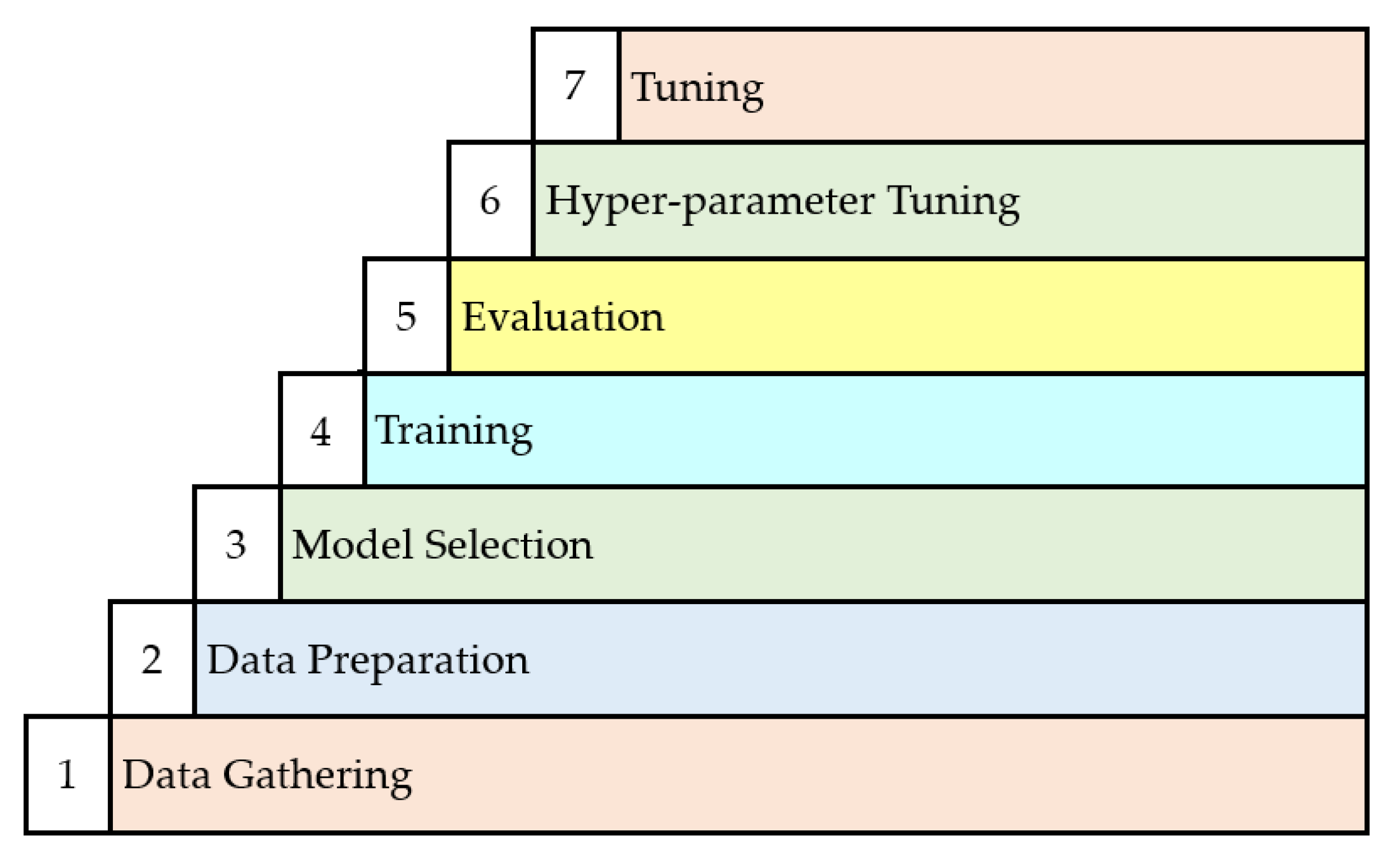
After data quality and confirmation issues were addressed, the interpretation of the DGA data commenced and a model was developed using the steps illustrated in Figure 2.
3.2. Main Notations
Table 1 expands the main abbreviations that have been used here.
3.3. Analysis of Dissolved Gases
One of the most prevalent technique for detecting progressing faults in transformers immersed in oil is gas analysis. DGA became an established art following the discovery in 1928 by Buchholz [32] that by extracting and studying dissolved gases generated during a progressively deteriorating condition in oil-filled transformers, one is be able to detect the problem with adequate precision. Since the gases formed in the course of a slow evolution of faults are dissolved in oil, extracting and analyzing these dissolved gases can foretell the onset of incipient fault condition [7,8,19]. Faults that are identifiable through DGA include corona discharge, heating of the core, arcing, and partial discharge. This early detection of emergent faults not only results in appreciable cost savings but also in intangible benefits such the timely decommissioning of faulty transformer units whose continued use may be risky. Additionally, early detection of emergent faults allows personnel to create a maintenance outage schedule for units in a precautionary state and document anomalies for newly purchased units under warranty. Cost saving is attained by preventing or alleviating damage to the transformer [12].
DGA, which discriminates against normal and abnormal conditions, is founded on the premise that an oil-immersed transformer in proper working conditions generates little or no fault gases. The DGA process begins with the collection oil samples from the transformer. The samples are then subjected to tests and procedures to determine the identity and quantity of liquefied gases [8]. Gases of interest for DGA analysis that are typically found dissolved in oil comprise ethane (C2H6), ethylene (C2H4), oxygen (O2), methane (CH4), acetylene (C2H2), nitrogen (N2) and hydrogen (H2). Fault gases can be categorized into three [7,8,33,34,35,36,37,38] namely;
- Hydrogen gas and hydrocarbons: H2, CH4, C2H2, C2H4
- Carbon oxides: CO2 and CO
- Non-fault gases: N2 and O2
The quantity and ratios of these gases will vary depending on whether a fault is developing in the transformer or not. A critical evaluation of the variation of gases present can precisely determine the underlying condition and the extent to which internal damages have been occasioned [39]. The leading causes of gas formation within an in-service transformer are either of thermal or electrical origins. DGA not only detects and identifies possible faults, but also improves the safety and reliability of the equipment while minimizing maintenance cost [23]. Typical faults that manifest in in-service transformers have been identified in [12,40,41] as follows;
- Partial Discharge (PD)—A partial discharge occurs when a confined section of a solid or fluid insulation material under high voltage stress experiences a partial collapse but does not entirely seal the space in between two conducting materials. In our context, the term PD refers only to corona PDs occurring in gas bubbles or voids as explained in [40].
- Energy Discharges—Energy discharge is the creation of a local conducting path or short circuit between capacitive stress grading foils that creates sparking around loose connections.
- Thermal Faults—refers to the circulation of electric current in insulating paper that result from excessive dielectric losses. These losses are themselves associated with moisture or an improperly selected insulating material that result in excessive dielectric temperatures.
The faults described above may manifest themselves in different ways as described in Table 2.
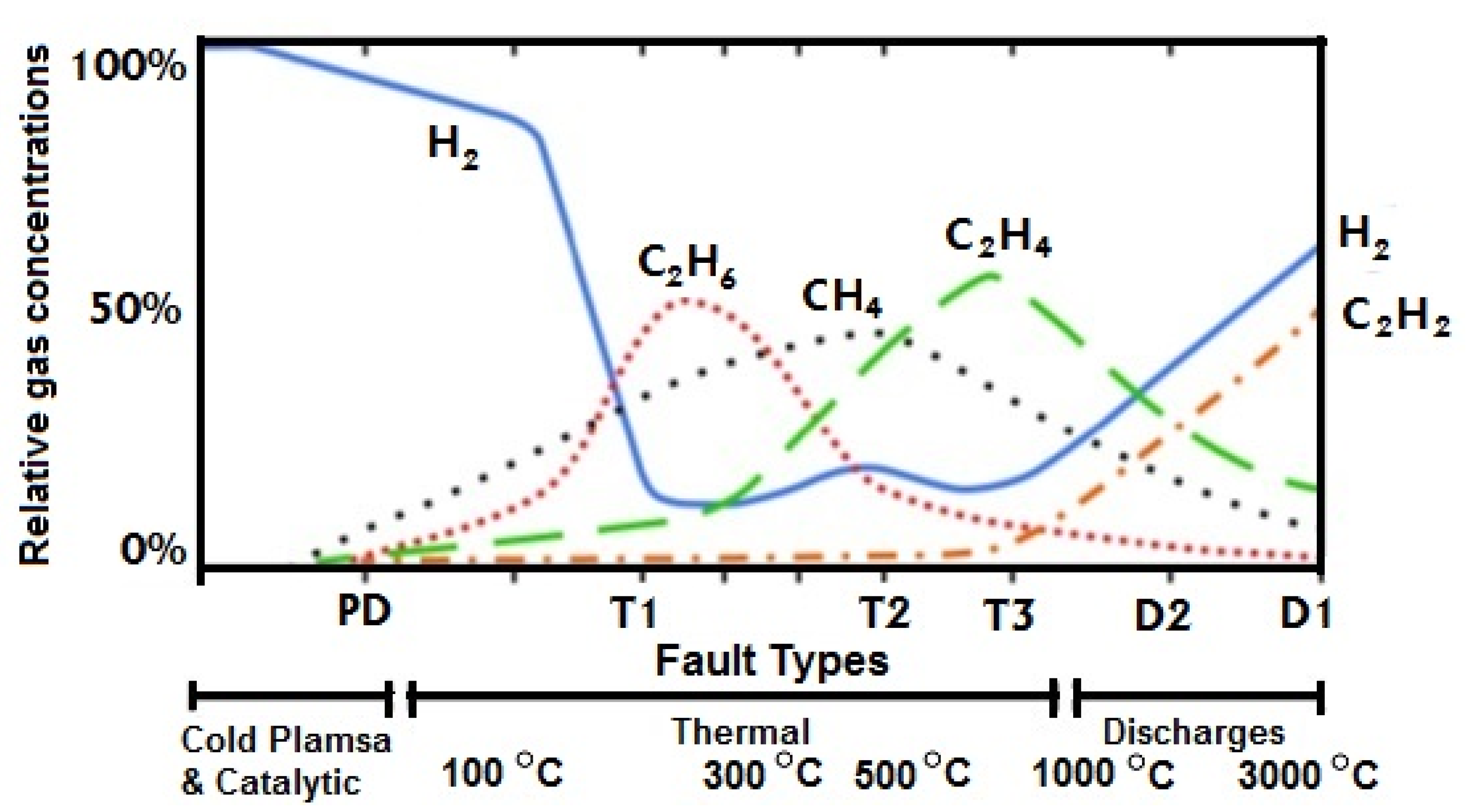
When mineral oil heats up to between 150–500 °C, methane, ethane, ethylene, and hydrogen are formed in varying quantities. As the temperature rises to exceed 500 °C, acetylene is generated in large quantities [16,17]. In the presence of high temperatures, paper insulation, and other solid insulating materials are known to produce carbon monoxide. At temperatures lower than 300 °C, carbon dioxide is produced.
Gas chromatography isolates each dissolved gas from all others making it possible to analyze and measure their individual concentrations. [41] provides standard procedures for collecting samples of oil from transformers and [42] details the analytical laboratory processes that separate and measure gas concentrations.
The IEEE [12], Conseil International des Grands Réseaux Électriques (CIGRÉ) [43] and The International Electrotechnical Commission (IEC) [40] are reputable international organizations that have separately drawn technical guidelines used to interpret DGA results. As seen in [12,40,41] each fault has a distinct signature in terms of the quantity and combination of the various fault gases. This distinction makes it possible to detect impending or active faults. Further to this, the particular combination of gases generated depends on the energy level and temperature at the location of the fault. High energy levels tend to produce higher temperatures. High temperatures in turn result in an accelerated rate of production of gases.
Figure 3 shows how the temperature influences the production of gases at various temperatures and the faults they are likely to suggest.
3.4. The Data Set
An exhaustive analysis of the data was carried through data exploration. Exploratory Data Analysis (EDA) is a preprocessing procedure used on raw data to obtain additional insight about the data before engaging in model building and training. During the EDA, the investigator is interested in knowing the shape of the data, the number of features it contains and the types of variables therein. EDA techniques are ran on raw data to extract its essential characteristics, define feature variables and obtain guidance on the selection of machine-learning algorithms [44,45,46]. To understand the data fully, multiple exploratory techniques are used, and the results aggregated. Figure 4 shows the contemporary methods employed in EDA and which have been used in this work.
Univariate visualization provides statistics for each parameter and is visualized in a one-dimensional space. Bivariate visualization determines the relationship that exist between each variable in the dataset and the dependent variable. Multivariate visualization aids in the identification of existing interactions between different fields in the dataset and examines the variables for correlation. Dimensionality reduction is a technique used to identify the most critical predictors so that the model is built using the minimum number of predictors required to maintain high accuracy [44,45,46].
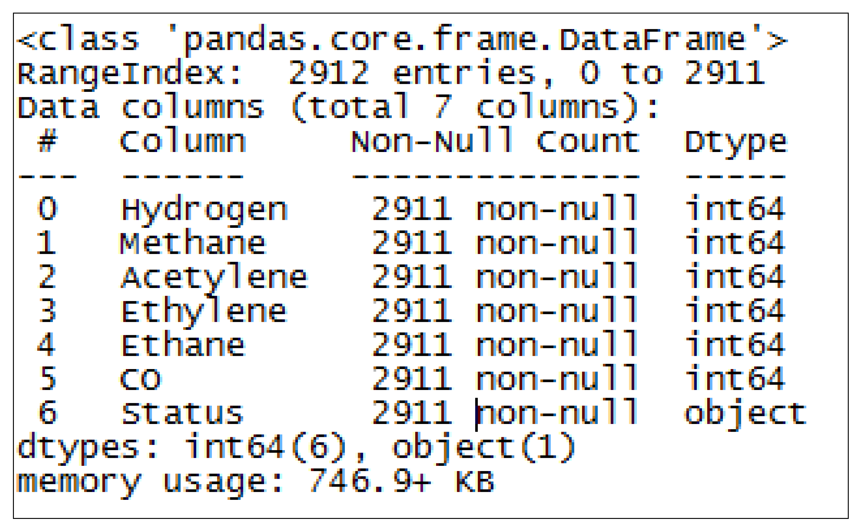
Figure 5 shows the type and number of variables in the dataset. The variable “Status” is the dependent variable and is of a categorical type while the rest are integers. The total number of observations for each were 2912 entries.
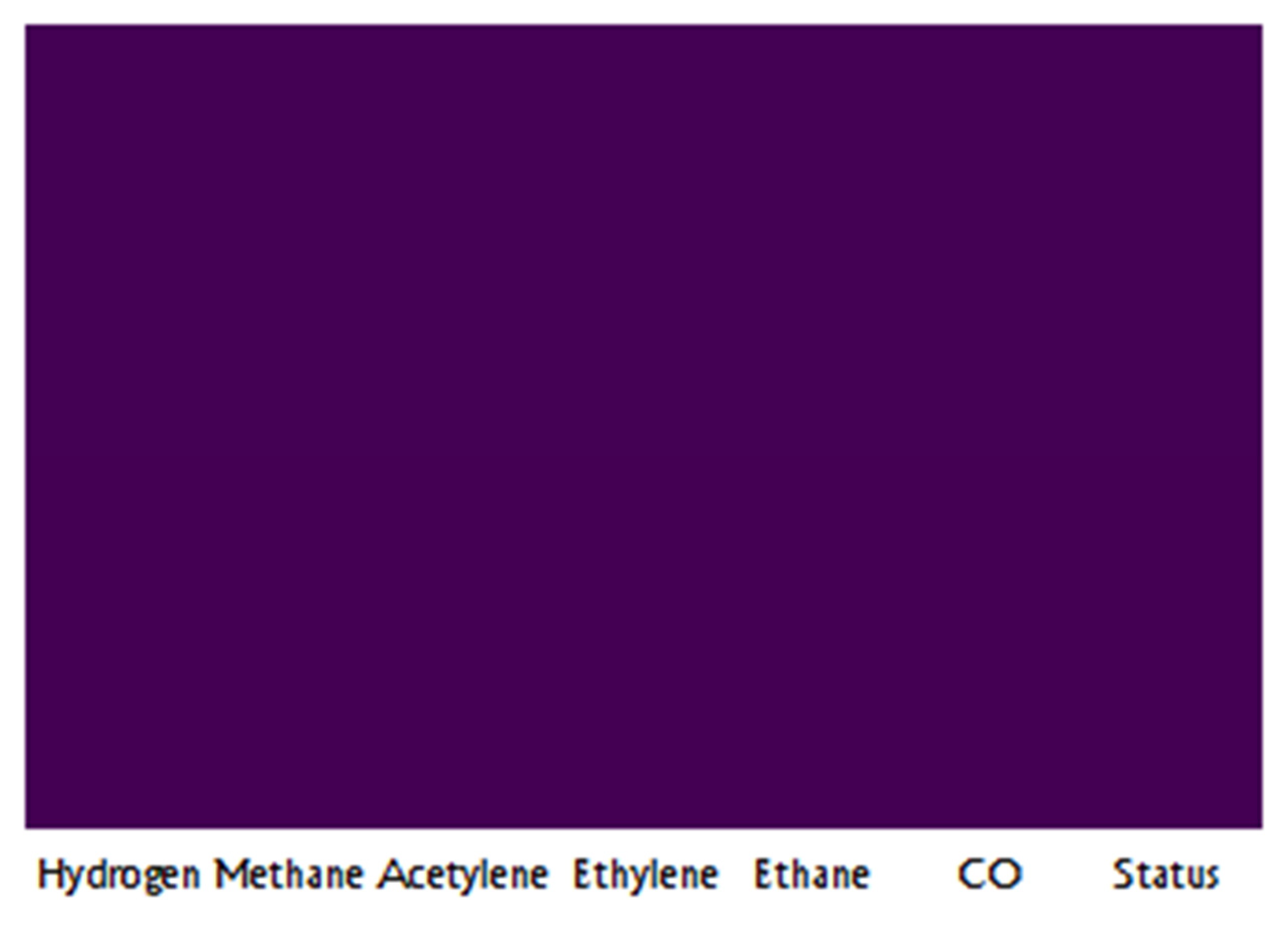
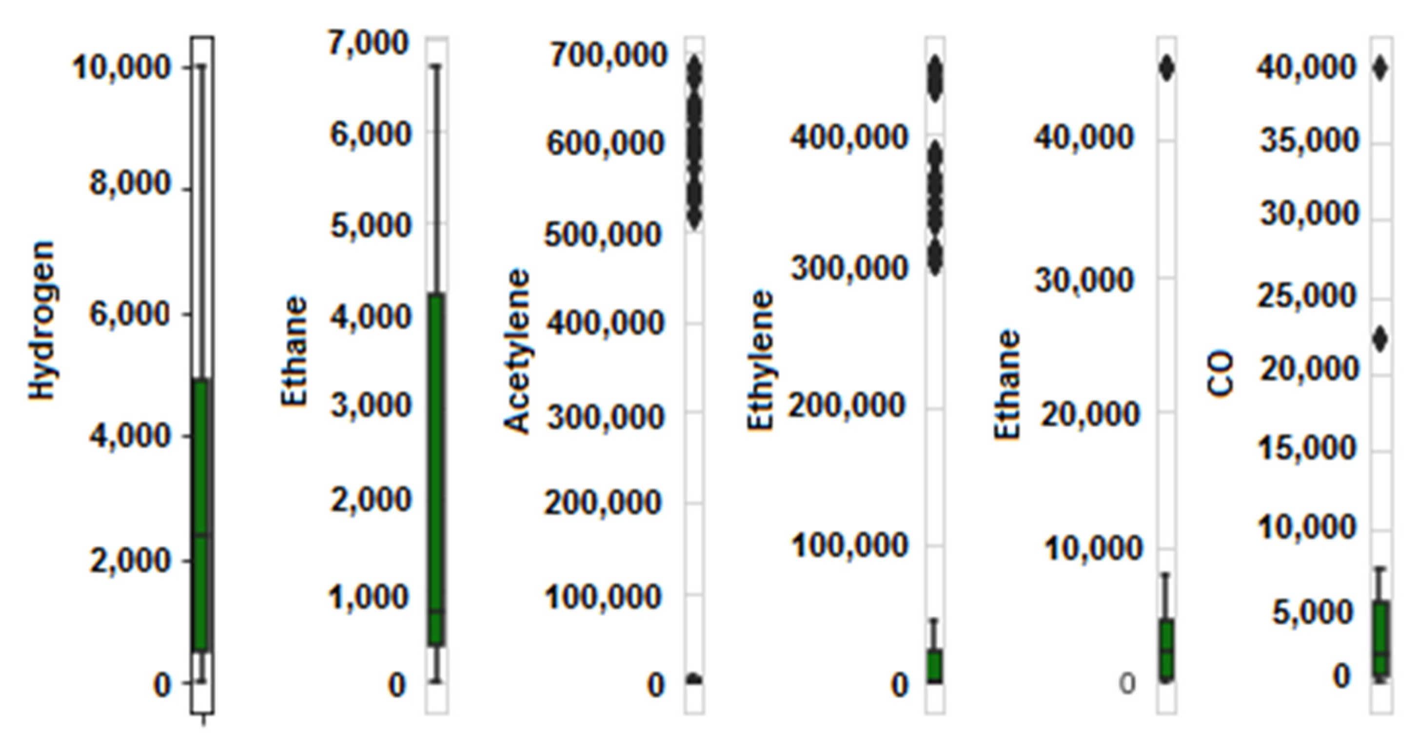
Primarily, the data was investigated for missing values. Figure 6 shows that there are no missing values. Whenever missing values exist, the columns affected show discontinuous gaps. In this case, the columns are continuous indicating that there are no missing values. Next, a box-and-whisker plot was created as shown in Figure 7. It suggests that the variables, acetylene and ethylene, have several outlying points above the outer whisker while hydrogen (H2), and carbon monoxide (CO) have no outliers. Outliers are normally handled by prediction or imputation (using the mean, mode and median) but by looking at the data, it is difficult to conclude that the outliers are as a result of human or mechanical error [47,48,49]. Therefore, the outliers were left as they were. It becomes imperative to handle outliers when it is evident that they result from errors committed during data collection or entry.
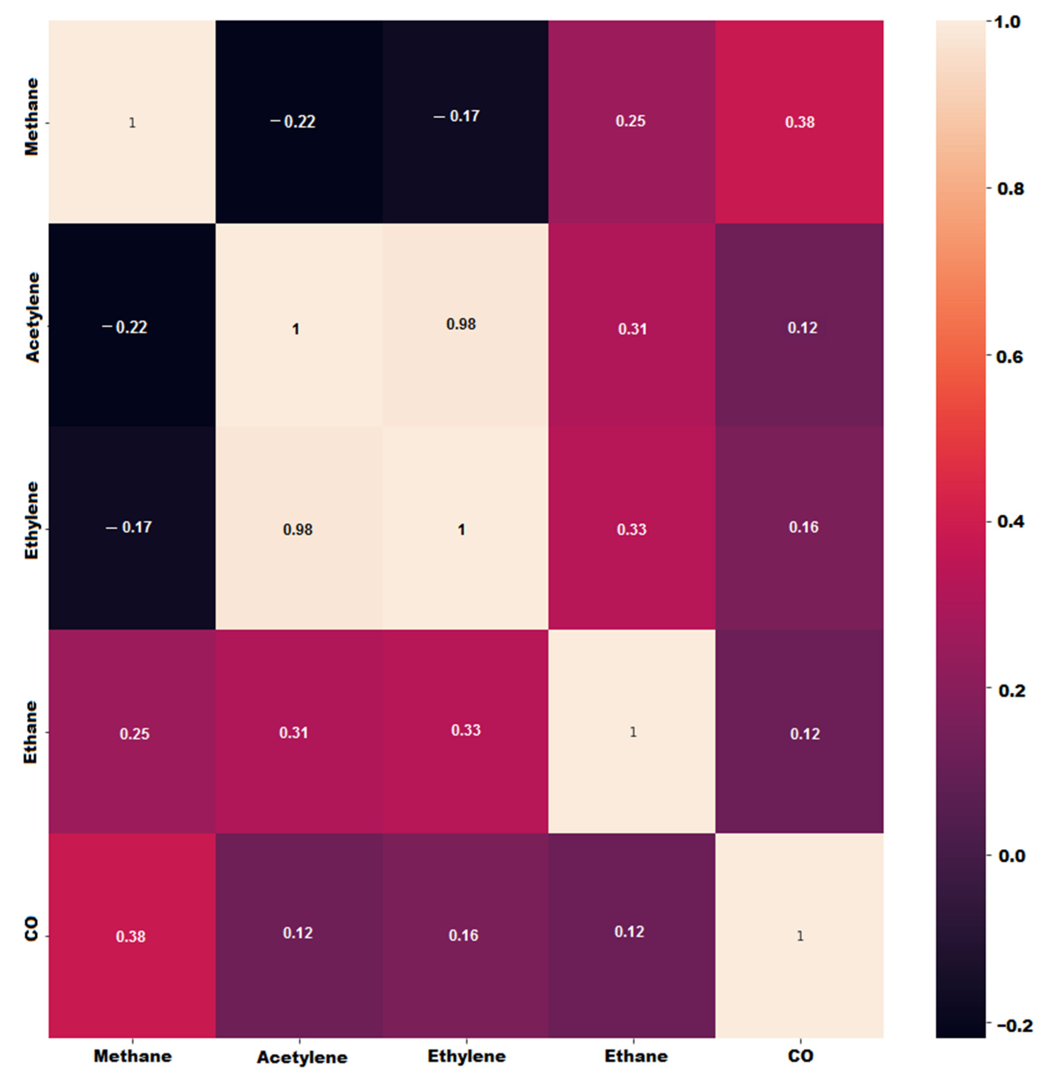
The correlation matrix or heat-map shown in Figure 8 establishes the correlation between the various pairs of variables from where it is determined that the correlation between the two variables, acetylene and ethylene, is high. A keen consideration of Figure 3 reveals that this correlation occurs in a coincidental manner because as the temperature rises there is a parallel increased production of both gases in slightly differing quantities. It is, therefore, concluded that this correlation does not imply causality [50].
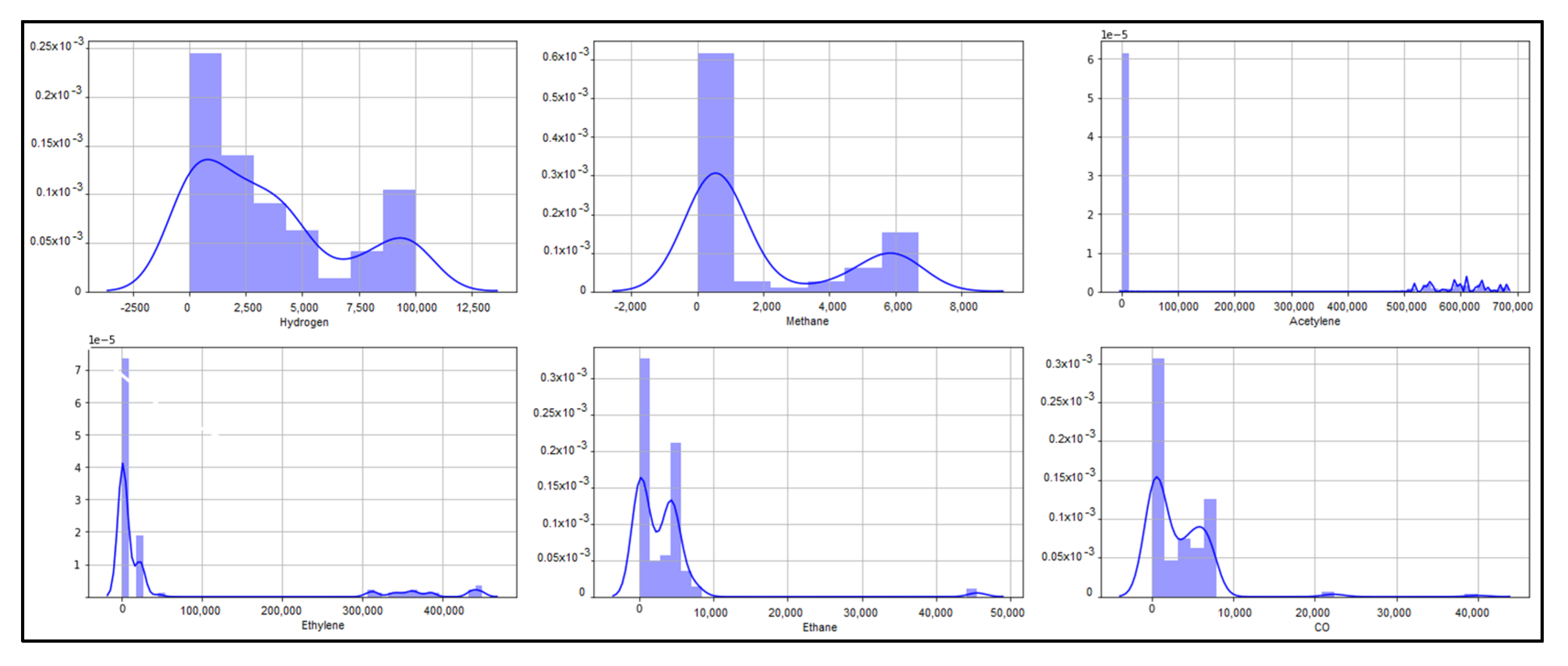
Figure 9 investigates the probability distribution of the variables. The variables hydrogen, methane, ethylene, ethane, and carbon monoxide appear to have a Gaussian distribution.
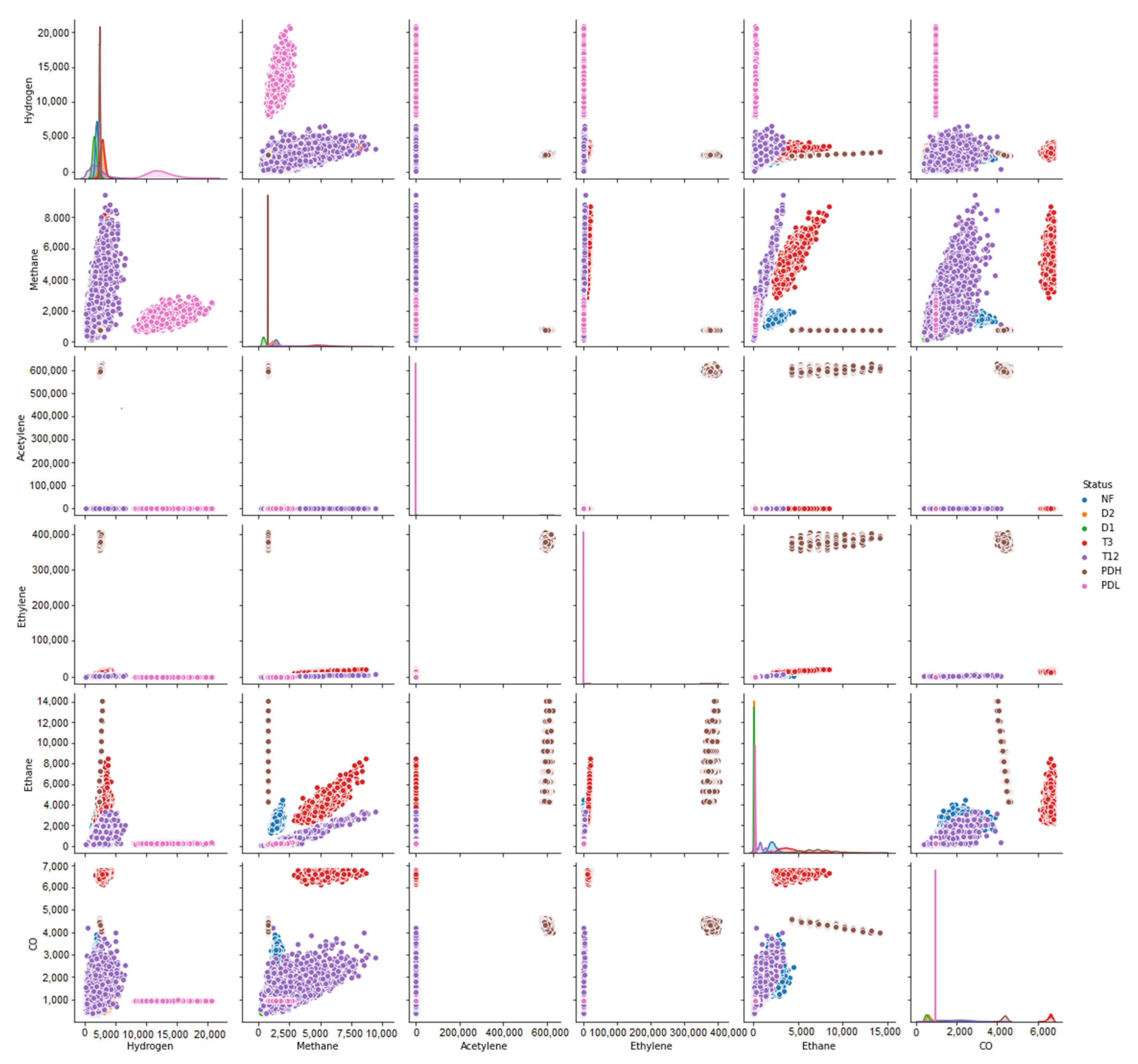
Figure 10 gives the pairs plot that visualizes the distribution of solitary input vectors and relationships between them. From Figure 10, we see that the variables pairs methane and ethane, and methane and hydrogen, are positively correlated. The same can be said about the variables methane and carbon monoxide.
3.5. Decision Trees (DT)
The DT algorithm is a machine learning method that estimates likelihood by developing a tree-like structure that repeatedly splits into smaller and smaller segments until it terminates in nodes called leaf nodes. The classification of data items in a decision tree is done through an iterative process of repeatedly questioning the features associated with the items [51,52,53]. The questions are enclosed in the nodes with each interior node pointing to a child node for every probable answer to its queries. In this manner, the queries create a hierarchically encoded tree structure.
The selection of the node on which the decision tree splits is done by examining its impurity. The impurity measures the similarity of the markers on a node and is implemented as the Gini Index or information gain. By definition, the Gini Index is a measure of the differences between the probability distributions of the dependent attribute values and divides the node in a manner that gives the smallest amount of impurity while the impurity measure used by the information gain is the entropy quantity. The node upon which a split is caused must result in the most amount of information gain. Equation (2) gives the formula for information gain while Equation (3) gives the formula for Gini Index.
where P prediction models constructed on tree-based algorithms are stable, accurate, and easy to interpret. In addition, they map well to non-linear interactions and are highly adaptive in solving a diverse range of problems unlike linear models [52].
3.6. Naïve Bayes
Naïve Bayes is a principle used in classification algorithms based on the Bayes theorem that states that
Naïve Bayes works on the assumption that every feature is independent of all others hence its name, “Naïve Bayes”. One strength of the Naïve Bayes algorithm, however, is that it can be trained on very small datasets.
3.7. Gradient Boosting
The gradient boosting, invented by Jerome Friedman, is used for both regression and classification tasks. It operates by creating a model that comprises an ensemble of frail prediction models from decision trees. As with all other supervised learning algorithm, gradient boosting defines a loss function as shown in Equation (5) and attempts to lessen its effect.
where = ith target value,
= ith prediction, L
is a Loss function.
3.8. The k–Near Neighbors (k-NN)
k-NN is a pre-trained ML process that works by first learning on a labelled dataset and then classifying new objects by recalling the examples on which it was trained [25], [54,55,56]. k-NN hinges on the assumption that data points that are similar most often lie close to each other. The k in k-NN signifies the number of adjacent neighbors that are retrieved by the classifier and used to predict a new data point. A value for k must be chosen iteratively such that it is just right for the data. It must be seen to reduce the number of errors encountered while maintaining the algorithms ability to make accurate predictions [25].
The k-Nearest Neighbors classifier algorithm works in the following manner. If xtrain is a training set with labels ytrain, and given that a new instance xtest is to be classified:
- First look for the most related occurrences (say XNN) to xtest that are in Xtrain.
- Obtain the labels yNN for all the occurrences in XNN.
- Predict the label for xtest by relating the labels yNN.
A sample is categorized by determining the majority vote cast by its k-neighbors, with the sample being assigned to the most popular vote. The metric that is traditionally used is the Euclidean distance, which is calculated as shown in Equation (6).
where m, n are two observations in the Euclidean space.
The k-NN algorithm is easy to implement but performs poorly as the number of predictor variables increase [24].
3.9. Random Forests
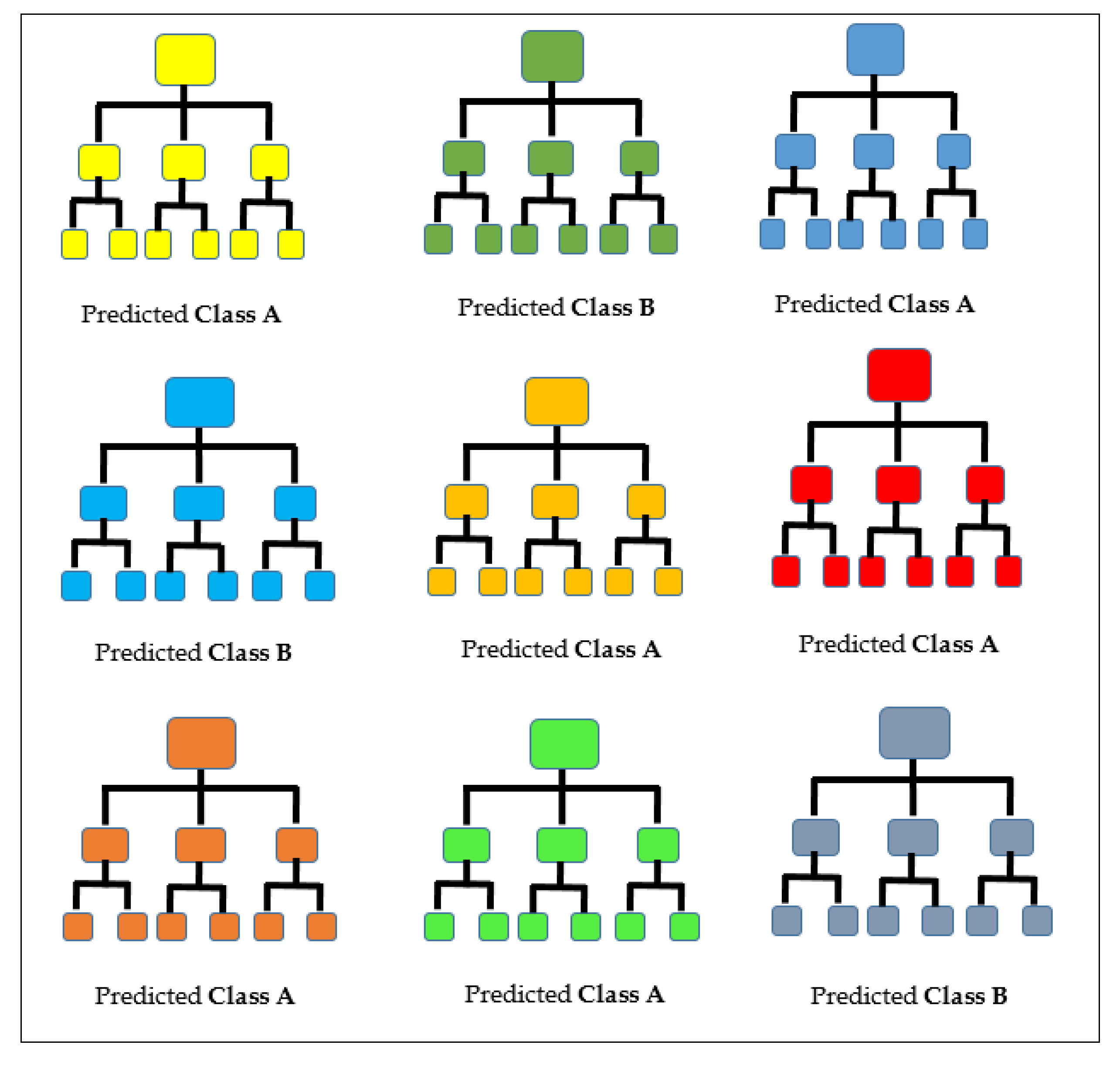
The Random Forest, also known as Random Decision Forest, presents a powerful way of exploring and analyzing data with the potential to perform predictive modeling. The Random Forest is made up numerous discrete decision trees that create a forest and hence the name Random Forest. The fundamental principle underlying the Random Forest is that individual constituent models cannot outperform numerous delinked trees working as a group. To make a prediction, each classifier in the assembly submits a prediction [57,58,59]. The votes are then tallied and the class that garners the highest ballots is presumed to be the prediction of the overall model as shown in Figure 11. Some of the reasons why the Random Forest is a powerful algorithm is that it does not suffer from overfitting and it is highly accurate, maintaining this accuracy even when some of the data is missing.
A Random Forest is defined as a class predictor made up of an ensemble of autonomous tree structures
where
are random vectors and
is the input vector [58]. A distinctive phenomenon of the Random Forest is that each tree is independent of all past random vectors but have a similar distribution. In creating the tree structures, a random attribute is selected upon which the split takes effect. The pool of potential attributes to split on is kept limited by calculating the first integer less than
[59].
In growing its trees, the Random Forest begins by first selecting randomly at each node a small group of input vectors on which to split then secondly it calculates a suitable split point. The best feature to split on is determined randomly.
The Random Forest algorithm works by executing the following three steps [60]:
- Selection of the set used for training. Using an indiscriminate sampling technique, several training sets are selected from the first dataset such that the magnitude of each is equal to that of the original.
- Construction a Random Forest model. For each of the bootstrap training set, a forest of classification trees is created to produce a similar number of decision trees.
- Form a simple voting. The training of the Random Forest can proceed simultaneously because the process of training its members is independent of each other, thus considerably enhancing its efficiency. To decide on some sample input, every decision tree submits a vote. The Random Forest algorithm decides the ultimate category of the submitted sample in accordance to the voting pattern.
3.10. KosaNet
KosaNet is designed as an ensemble-based machine-learning technique that improves upon the decision tree algorithm by creating a semblance of an electoral college where decisions are made by a majority vote. KosaNet hinges on the notion that when many separate and independent entities vote in a particular direction, they are highly likely to be correct [61]. The electoral college operates like a democracy where the minority have their say and the majority their way. The vote of the majority constitutes the prediction of the model. To minimize the variance of our predictions, several classifiers modeled on separate sub-samples of the same data set were built. The results of the vote by the separate classifiers are tallied and the majority vote determined which then constitute the prediction of the model.
4. Experiments and Model Evaluation
To implement the KosaNet model, Python programming environment is used. After the model was implemented, its performance was evaluated. Several metrics were considered for this purpose. This section outlines how the model was implemented and explains the evaluation metrics used in its assessment.
4.1. Implementation Environment, Cost, and Complexity
KosaNet has been implement in the Python programming environment. Apart from being completely open source, Python boasts of a rich set of libraries that support data analytic and analysis [62]. In addition, Python has a comfortable learning curve for programming novices [63]. The specific libraries that were used in conjunction with Python are Matplotlib, Numpy, Pandas, Seaborn, Keras, Tensorflow and Scikit-Learn [44,45,62,64,65].
The proposed framework is a cloud-based solution. The proposed algorithm shall reside on a cloud-based server machine. This server shall not only perform DGA data interpretation but shall also aggregate the data received from the sensors. The computational complexity of the proposed framework is
during training and
during prediction as suggested in [66].
4.2. Classification Evaluation Metrics
Multiple methods exist for the performance evaluation of classifier algorithms. Subsequent sections present a detailed discourse on the evaluation metrics that were employed in this study.
4.2.1. Confusion Matrix (CM)
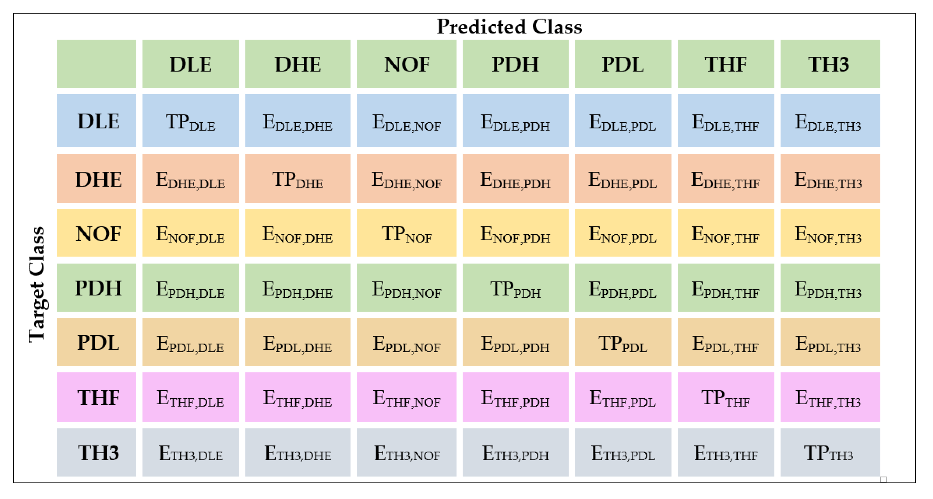
The CM is an arithmetically derived means of quantifying how well a model performs during classification. It gives a comprehensive and complete picture of how the classifier performed, where it went wrong and offers guidance on how to correct the situation. It is basically an N by N-dimensional table that compares the “Actual” versus the “Predicted” entries [67,68,69]. In this case, N = 7 representing the various classes available in the data set and it shows the definite positives, definite negatives, projected positives, and projected negatives. The running diagonal represents the values of the correctly predicted instances and is also known as true positive (TP). The values in the off diagonal represents the incorrectly classified instances and manifest as falsely positive or falsely negative. The falsely positive are referred to as the Type I errors while the falsely negative instances are Type II errors.
4.2.2. Classification Accuracy
4.2.3. Classification Error
The classification error provides an indication of how often the classifier is incorrect [70,71,72,73,74,75,76] and is calculated using Equation (8).
where trp, trn, fap, and fan denotes the factual positive, factual negative, erroneous positive, erroneous negative respectively, for every class x such that x∈{x:y}.
4.2.4. Averaged Instance Sensitivity
The sensitivity, also referred to as the recall, is an intuitive measure of how sensitive the classifier is to detecting faults whenever they occur [70,71,72,73,74,75,76]. The averaged sensitivity is obtained as shown in Equation (9)
where trnj refers to the true negative rate for class j, trpj is true positive rate for class j while ej,x represents the classification error where class j is incorrectly classified as class x.
4.2.5. Averaged Precision
Average precision answers the question of how often a prediction is correct when a positive value is foretold from the aggregate prediction patterns in an affirmative class. [70,71,72,73,74,75,76]. The precision is calculated per class then averaged as shown in Equation (10).
4.2.6. Averaged F1 Score
5. Evaluation and Results
The results of the evaluation of KosaNet vis-à-vis other multinomial classifiers models are presented and discussed based on the metrics discussed previously in Section 4.2.
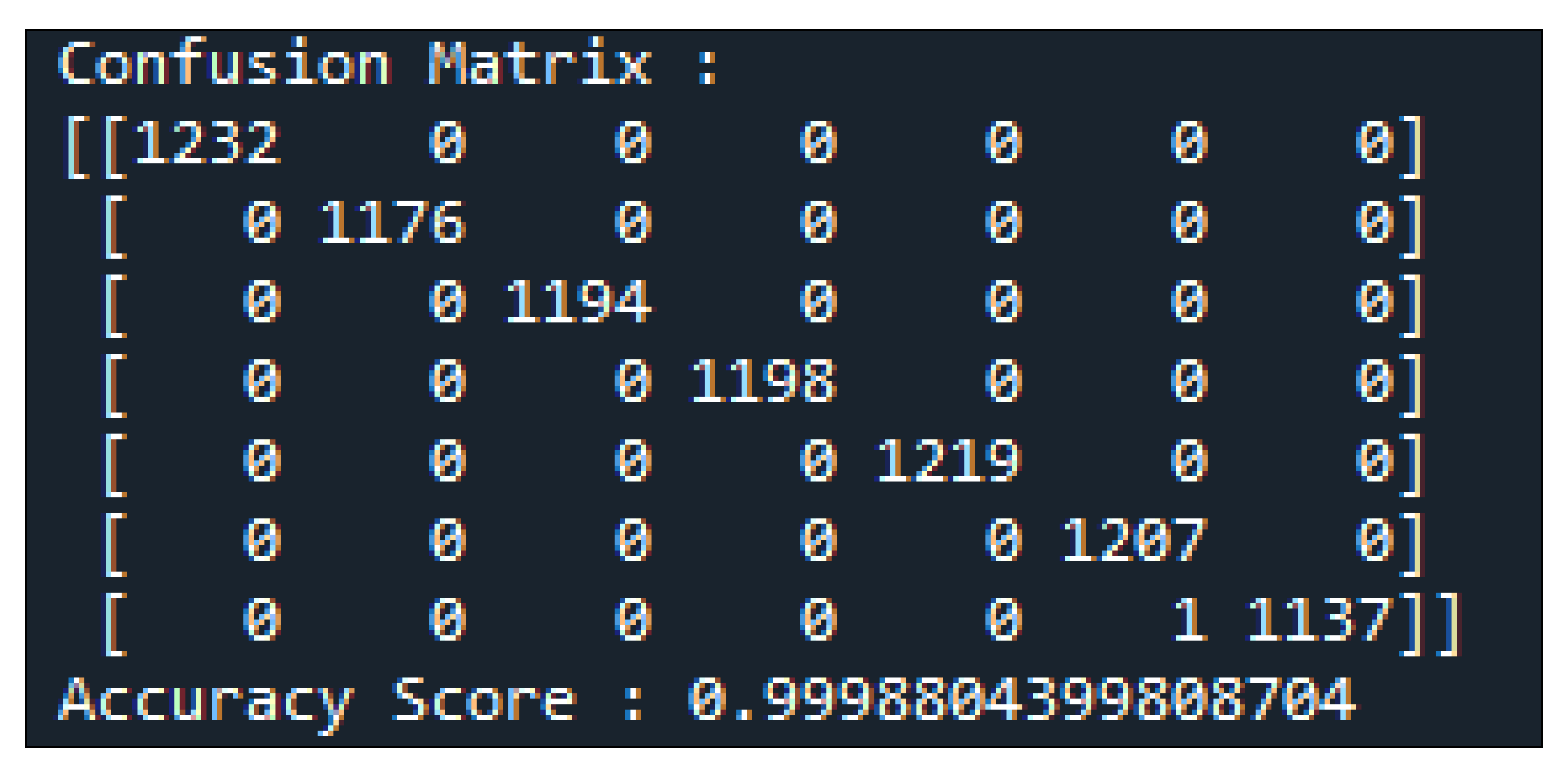
Figure 13 shows the confusion matrix that was obtained from the KosaNet model.
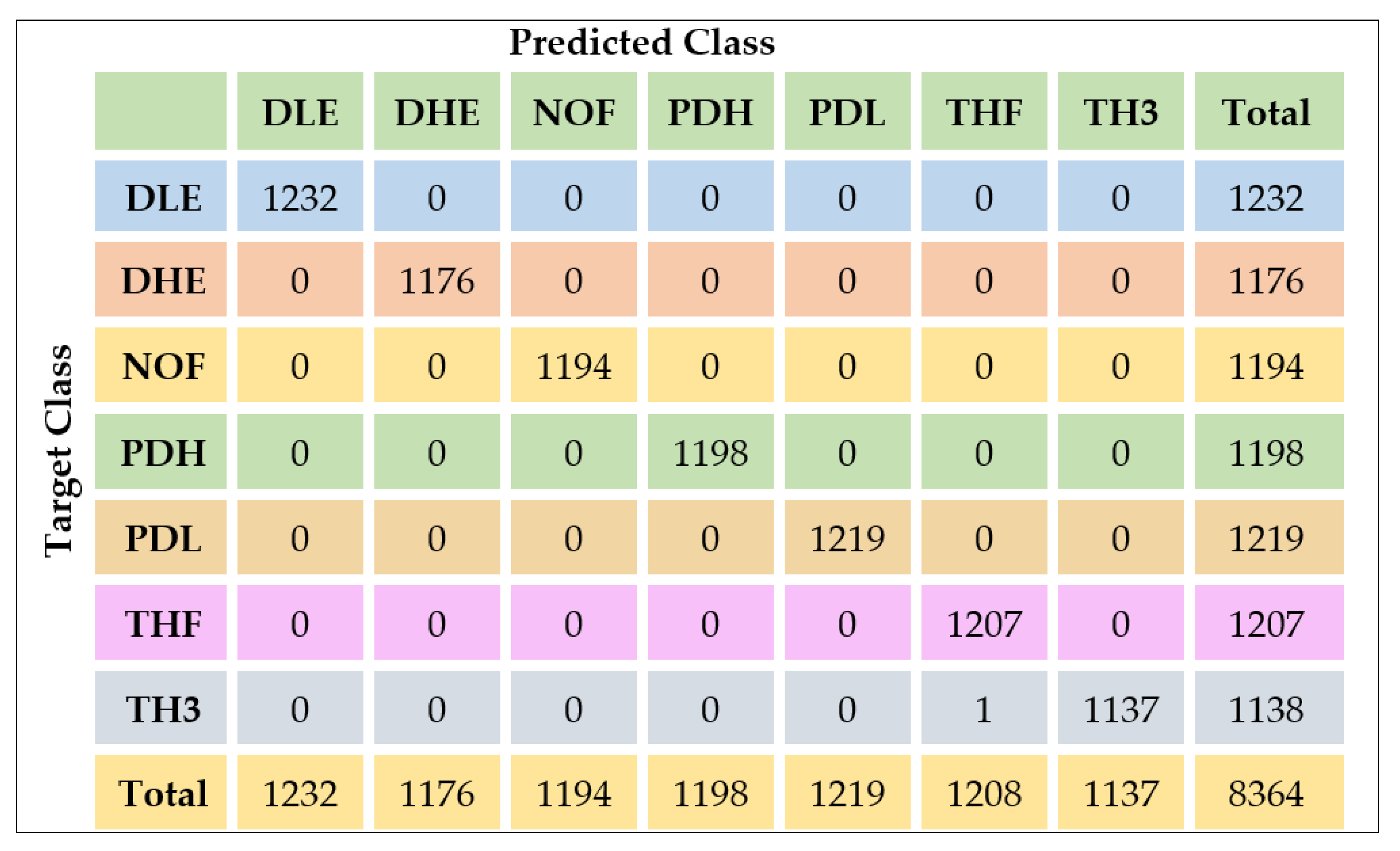
The label encoder assigned the columns in the following order: DLE, DHE, NOF, PDH, PDL, THF, and TH3. To facilitate further discussion, the confusion matrix has been decomposed as shown in Figure 14.
In Figure 14, an additional row and column for tabulating the total has been included to allow us to compute evaluation metrics discussed in Section 4.2. The confusion matrix enables us to calculate the classification accuracy, classification error, sensitivity, precision and the f1-score [70,71,72,73,74,75,76,77]. Table 3 is an extract of the DGA data in ppm that was used to evaluate the model.
Table 4 shows how classical techniques compare against the proposed model. The incorrectly labelled classes are marked in red.
In Table 4, a comparison of classification results using Key Gases, Duval Triangle, Nomography, and KosaNet is made. These results show that the Key Gases method correctly classified 18 out of 20 or 90%. This performance was replicated by the Duval triangle method that also correctly classified 90%. The Nomography technique had the least accuracy attaining only 85%. In comparison, KosaNet attained an accuracy of 95% of accurately classified instances. Table 5 provides the results obtained when the model is compared against other algorithms with multiclass classification ability.
As seen in Table 5, the decision tree, Naïve Bayes, gradient boosting, k-NN, random Forest, and KosaNet realized an accuracy of 68.5%, 70%, 83%, 89.7% 92.4% and 99.9% respectively. This implies that with KosaNet, less than 1 out of 10 labels are incorrectly labelled. With KosaNet, the precision value was high with an implication that more than 9 out of 10 labels are incorrectly classified. Similarly, the recall value of 99.9% means that less than 1 out of 10 DGA readings are incorrectly labelled. The f1 score, which helps preserve a balance between precision and recall, tends towards one, which is an excellent value for this metric [14].
6. Conclusions and Future Work
This manuscript endorses an intuitive DGA interpretation algorithm christened KosaNet is proposed. Actual DGA data was obtained from Kenya Power Ltd., the sole utility power company in Kenya. The dataset was used to build and evaluate the performance of KosaNet vis-à-vis other algorithms with multinomial classification abilities. Experimental results have shown that KosaNet has superior classification ability particularly for multiclass DGA data. With a classification accuracy of 99.98%, KosaNet would greatly enhance the detection of incipient power transformer faults hence giving technicians and managers the opportunity to plan for reparative maintenance. The deployment of KosaNet has the potential to increase network uptime by more than 75%, resulting in fewer disruptions to the supply of electrical energy. We advocate for the use of KosaNet in the analysis and classification of DGA data to enhance the early discovery of silently active fault s in transformers units.
In a future study, the authors will explore the use of KosaNet for time series data where IoT-enabled smart sensors will be deployed for real-time observation of transformers.
Author Contributions
Conceptualization, data collection, methodology, formal analysis, validation, software, investigation, and writing original draft, G.O.; writing, review, and editing, G.O., R.M. and D.H.; supervision, R.M. and D.H. All authors have read and agreed to the published version of the manuscript.
Funding
This research study received no funding.
Institutional Review Board Statement
Not applicable.
Informed Consent Statement
Not applicable.
Data Availability Statement
3rd Party Data Restrictions apply to the availability of these data. Data was obtained from Kenya Power Ltd. and are available from the authors upon request with the permission of Kenya Power Ltd.
Acknowledgments
G.O. thanks R.M. and D.H. for the tireless support. The seemingly endless cycle of reviewing and editing this manuscript is highly appreciated. G.O. further thanks the management of Kenya Power Ltd. for providing the data used in this work.
Conflicts of Interest
The authors have no conflict of interest to declare.
Abbreviations
| ANN | Artificial Neural Network |
| CIGRÉ | Conseil International des Grands Réseaux Électriques |
| CD | Cellulose Decomposition |
| DLE/D1 | Low Energy Discharge (Sparking) |
| DHE/D2 | High Energy Discharge (Arcing) |
| DGA | Dissolved gas analysis |
| DPM | Duval Pentagon Method |
| DSO | Distributed System Operator |
| EDA | Exploratory Data Analysis |
| emf | electromotive force |
| FN | False Negatives |
| FP | False Positives |
| H2 | Hydrogen |
| IEC | International Electrotechnical Commission |
| IEEE | The Institute of Electrical and Electronics Engineers |
| kNN | k-Nearest Neighbor |
| MLP | multilayer perceptron |
| N2 | Nitrogen |
| O2 | Oxygen |
| PD | Partial Discharge |
| ppm | Parts Per Million |
| PSO | Particle Swarm Optimization |
| PTD | Partial Discharge |
| RF | Random Forests |
| ROC | Region of Certainty |
| SVM | Support Vector Machine |
References
- Grigsby, L.L. Electric Power Generation, Transmission, and Distribution, 3rd ed.; CRC Press: Boca Raton, FL, USA, 2012. [Google Scholar]
- Ndungu, C.; Nderu, J.; Ngoo, L.; Hinga, P. A Study of the Root Causes of High Failure Rate of Distribution Transformer—A Case Study. Int. J. Eng. Sci. 2017, 6, 14–18. [Google Scholar] [CrossRef]
- Wang, L. The Fault Causes of Overhead Lines in Distribution Network. Int. Semin. Appl. Phys. Optoelectron. Photonics 2017, 61, 02017. [Google Scholar] [CrossRef] [Green Version]
- Abotsi, A.K. Power Outages and Production Efficiency of Firms in Africa. Int. J. Energy Econ. Policy 2016, 6, 98–104. [Google Scholar] [CrossRef] [Green Version]
- Sarma, J.J.; Sarma, R. Fault analysis of High Voltage Power. Int. J. Adv. Res. Electr. Electron. Instrum. Eng. 2017, 6, 2411–2419. [Google Scholar]
- Sun, H.C.; Huang, Y.C.; Huang, C.M. A review of dissolved gas analysis in power transformers. Energy Procedia 2012, 14, 1220–1225. [Google Scholar] [CrossRef] [Green Version]
- Chakravorti, S.; Dey, D.; Chatterjee, B. Recent Trends in the Condition Monitoring of Transformers; Springer: London, UK, 2013. [Google Scholar]
- Ranjan, S.; Narayana, P.L.; Kirar, M. Dissolved Gas Analysis based Incipient Fault Diagnosis of Transformer: A Review. Impending Power Demand Innov. Energy Paths 2015, 1, 325–332. [Google Scholar]
- Theraja, B.L.; Theraja, A.K. A Textbook of Electrical Technology; S Chand & Co Ltd.: Uttar Pradesh, India, 1999; Volume 1. [Google Scholar]
- Turkar, R.; Shahare, R.; Sidam, P.; Giradkar, V.; Patil, A.; Sarode, P. Design and fabrication of a Single-phase 1KVA Transformer with automatic cooling system. Int. Res. J. Eng. Technol. 2018, 5, 679–682. [Google Scholar]
- Nickelson, L. Electromagnetic Theory and Plasmonics for Engineers; Springer: Singapore, 2019. [Google Scholar]
- IEEE-C57.104. IEEE Guide for the Interpretation of Gases Generated in Mineral Oil-Immersed Transformers; IEEE: New York, NY, USA, 2019. [Google Scholar]
- Hartnack, M. Rising Power Outage Cost and Frequency Is Driving Grid Modernization Investment. Navig. Res. 2018. Available online: https://www.navigantresearch.com/news-and-views/rising-power-outage-cost-and-frequency-is-driving-grid-modernization-investment (accessed on 27 December 2020).
- Africa Energy Series: Kenya Special Report; Invest in the Energy Sector of Kenya: Nairobi, Kenya, 2020.
- Apte, S.; Somalwar, R.; Wajirabadkar, A. Incipient Fault Diagnosis of Transformer by DGA Using Fuzzy Logic. In Proceedings of the 2018 IEEE International Conference on Power Electronics, Drives and Energy Systems (PEDES), Chennai, India, 18–21 December 2018; pp. 1–5. [Google Scholar]
- Soni, R.; Joshi, S.; Lakhiani, V.; Jhala, A. Condition Monitoring of Power Transformer Using Dissolved Gas Analysis of Mineral Oil: A Review. Int. J. Adv. Eng. Res. Dev. 2015, 3, 2348–4470. [Google Scholar]
- Faiz, J.; Heydarabadi, R. Diagnosing power transformers faults. Russ. Electr. Eng. 2014, 85, 785–793. [Google Scholar] [CrossRef]
- Bage, M.; Bisht, P.S.; Khanna, A. Transformer Fault Diagnosis Based on DGA using Classical Methods. Int. J. Eng. Res. Technol. 2016, 4, 1–7. [Google Scholar]
- Abu-Siada, A. Improved consistent interpretation approach of fault type within power transformers using dissolved gas analysis and gene expression programming. Energies 2019, 12, 730. [Google Scholar] [CrossRef] [Green Version]
- Prasojo, R.A.; Gumilang, H.; Suwarno; Maulidevi, N.U.; Soedjarno, B.A. A fuzzy logic model for power transformer faults’ severity determination based on gas level, gas rate, and dissolved gas analysis interpretation. Energies 2020, 13, 1009. [Google Scholar] [CrossRef] [Green Version]
- Malik, H.; Sharma, R.; Mishra, S. Fuzzy reinforcement learning based intelligent classifier for power transformer faults. ISA Trans. 2020, 101, 390–398. [Google Scholar] [CrossRef] [PubMed]
- Chatterjee, K.; Dawn, S.; Jadoun, V.K.; Jarial, R.K. Novel prediction-reliability based graphical DGA technique using multi-layer perceptron network & gas ratio combination algorithm. IET Sci. Meas. Technol. 2019, 13, 836–842. [Google Scholar]
- Bustamante, S.; Manana, M.; Arroyo, A.; Castro, P.; Laso, A.; Martinez, R. Dissolved Gas Analysis Equipment for online monitoring of transformer oil: A review. Sensors 2019, 19, 4057. [Google Scholar] [CrossRef] [Green Version]
- Benmahamed, Y.; Kemari, Y.; Teguar, M.; Boubakeur, A. Diagnosis of Power Transformer Oil Using KNN and Naïve Bayes Classifiers. In Proceedings of the 2018 IEEE 2nd International Conference on Dielectrics ICD, Budapest, Hungary, 1–5 July 2018; pp. 1–4. [Google Scholar]
- Tanfilyeva, D.V.; Tanfyev, O.V.; Kazantsev, Y.V. K-nearest neighbor method for power transformers condition assessment. IOP Conf. Ser. Mater. Sci. Eng. 2019, 643, 012016. [Google Scholar] [CrossRef]
- Parejo, A.; Personal, E.; Larios, D.F.; Guerrero, J.I.; García, A.; León, C. Monitoring and Fault Location Sensor Network for Underground Distribution Lines. Sensors 2019, 19, 576. [Google Scholar] [CrossRef] [Green Version]
- Illias, H.A.; Chai, X.R.; Bakar, A.H.A.; Mokhlis, H. Transformer incipient fault prediction using combined artificial neural network and various particle swarm optimisation techniques. PLoS ONE 2015, 10, e0129363. [Google Scholar] [CrossRef]
- Illias, H.A.; Liang, W.Z. Identification of transformer fault based on dissolved gas analysis using hybrid support vector machine-modified evolutionary particle swarm optimisation. PLoS ONE 2018, 13, e0191366. [Google Scholar] [CrossRef] [Green Version]
- Liu, Y.; Song, B.; Wang, L.; Gao, J.; Xu, R. Power transformer fault diagnosis based on dissolved gas analysis by correlation coefficient-DBSCAN. Appl. Sci. 2020, 10, 4440. [Google Scholar] [CrossRef]
- Pattanadech, N.; Sasomponsawatline, K.; Siriworachanyadee, J.; Angsusatra, W. The conformity of DGA interpretation techniques: Experience from transformer 132 units. In Proceedings of the 2019 IEEE 20th International Conference on Dielectric Liquids (ICDL), Roma, Italy, 23–27 June 2019; pp. 1–4. [Google Scholar]
- Borcard, D.; Gillet, F.; Legendre, P. Numerical Ecology with R; Springer International Publishing AG: Manhattan, NY, USA, 2018. [Google Scholar]
- Bin, N.; Bakar, A. A New Technique to Detect Loss of Insulation Life in Power Transformers. Ph.D. Thesis, Curtin University, Perth, Australia, 2016. [Google Scholar]
- Bakar, N.A.; Abu-Siada, A.; Islam, S. A Review of Dissolved Gas. Deis Featur. Artic. 2014, 30, 39–49. [Google Scholar]
- Sisic, E. Chromatographic analysis of gases from the transformer. Transform. Mag. 2015, 2, 36–41. [Google Scholar]
- Ravichandran, N.; Jayalakshmi, V. Investigations on power transformer faults based on dissolved gas analysis. Int. J. Innov. Technol. Explor. Eng. 2019, 8, 296–299. [Google Scholar]
- Duval, M. A review of faults detectable by gas-in-oil analysis in transformers. In IEEE Electrical Insulation Magazine; IEEE: New York, NY, USA, 2002; Volume 18, pp. 8–17. [Google Scholar]
- Akbari, A.; Setayeshmehr, A.; Borsi, H.; Gockenbach, E.; Fofana, I. Intelligent agent-based system using dissolved gas analysis to detect incipient faults in power transformers. In IEEE Electrical Insulation Magazine; IEEE: New York, NY, USA, 2010; Volume 26, pp. 27–40. [Google Scholar]
- Golkhah, M.; Shamshirgar, S.S.; Vahidi, M.A. Artificial neural networks applied to DGA for fault diagnosis in oil-filled power transformers. J. Electr. Electron. Eng. Res. 2011, 3, 1–10. [Google Scholar]
- Huang, Y.C.; Huang, C.M.; Sun, H.C. Data mining for oil-insulated power transformers: An advanced literature survey. Wiley Interdiscip. Rev. Data Min. Knowl. Discov. 2012, 2, 138–148. [Google Scholar] [CrossRef]
- CIGRE-SC.15. Recent Developments on the Interpretation of Dissolved Gas Analysis in Transformers; Commission Electrotechnique Internationale: Geneva, Switzerland, 2006; Volume 296. [Google Scholar]
- IEC-60599. Mineral Oil-Filled Electrical Equipment in Service–Guidance on the Interpretation of Dissolved and Free Gases Analysis; IEC: Geneva, Switzerland, 2015. [Google Scholar]
- ASTM-D923-15. Standard Practices for Sampling Electrical Insulating Liquids; ASTM International: West Conshohocken, PA, USA, 2015. [Google Scholar]
- ASTM-D3612-02. Standard Test Method for Analysis of Gases Dissolved in Electrical Insulating Oil by Gas Chromatography; Conseil International des Grands Réseaux Électriques: Paris, France, 2017; Volume 5. [Google Scholar]
- Kumar, A. Master Data Science and Data Analysis With Pandas; Packt Publishing Ltd.: Birmingham, UK, 2020. [Google Scholar]
- Garg, H. Mastering Exploratory Analysis with Pandas; Packt Publishing Ltd.: Birmingham, UK, 2018. [Google Scholar]
- Larose, D.T.; Larose, C.D. Discovering Knowledge in Data: An Introduction to Data Mining; John Wiley & Sons, Inc.: Hoboken, NJ, USA, 2014. [Google Scholar]
- Mostafa, S.M. Imputing missing values using cumulative linear regression. CAAI Trans. Intell. Technol. 2019, 4, 182–200. [Google Scholar] [CrossRef]
- Niederhut, D. Safe handling instructions for missing data. In Proceedings of the Python in Science Conferences, Trento, Italy, 28 August–1 September 2018; pp. 56–60. [Google Scholar]
- Bertsimas, D.; Pawlowski, C.; Zhuo, Y.D. From predictive methods to missing data imputation: An optimization approach. J. Mach. Learn. Res. 2018, 18, 1–39. [Google Scholar]
- Devroop, K. Correlation versus Causation: Another Look at a Common Misinterpretation. Alberta J. Educ. Res. 2000, 41, 271–284. [Google Scholar]
- Basuki, A.; Suwarno. Online dissolved gas analysis of power transformers based on decision tree model. In Proceedings of the 2018 Conference on Power Engineering and Renewable Energy (ICPERE), Solo, Indonesia, 29–31 October 2018; pp. 1–6. [Google Scholar]
- Galitskaya, E.G.; Galitskkiy, E.B. Classification trees. Sotsiologicheskie Issled. 2013, 3, 84–88. [Google Scholar]
- Chiu, S.; Tavella, D. Introduction to Data Mining; Routledge: Oxfordshire, UK, 2008; pp. 137–192. [Google Scholar]
- Luo, X.; Yu, J.X.; Li, Z. Advanced Data Mining and Applications. In Proceedings of the 10th International Conference, ADMA, Guilin, China, 19–21 December 2014; Volume 8933. [Google Scholar]
- Zhang, Z. Introduction to machine learning: K-nearest neighbors. Ann. Transl. Med. 2016, 4, 218–226. [Google Scholar] [CrossRef] [PubMed] [Green Version]
- Imandoust, S.B.; Bolandraftar, M. Application of K-Nearest Neighbor (KNN) Approach for Predicting Economic Events: Theoretical Background. Int. J. Eng. Res. Appl. 2013, 3, 605–610. [Google Scholar]
- Gao, X.; Wen, J.; Zhang, C. An Improved Random Forest Algorithm for Predicting Employee Turnover. Math. Probl. Eng. 2019, 2019, 1–12. [Google Scholar] [CrossRef]
- Breiman, L. Random Forests. Mach. Learn. 2001, 45, 5–32. [Google Scholar] [CrossRef] [Green Version]
- Sug, H. Applying randomness effectively based on random forests for classification task of datasets of insufficient information. J. Appl. Math. 2012, 2012, 1–13. [Google Scholar] [CrossRef]
- Kaur, M.; Kalra, S. A Review on IOT Based Smart Grid. Int. J. Energy Inf. Commun. 2016, 7, 11–22. [Google Scholar] [CrossRef]
- Bakhtouchi, A. A Tree Decision Based Approach for Selecting Software Development Methodology. In Proceedings of the 2018 International Conference on Smart Communications in Network Technologies (SaCoNeT), Nice, France, 20–24 May 2018; pp. 211–216. [Google Scholar]
- Williams, E. Python for Data Science; O’Reilly Media, Inc.: Sebastopol, CA, USA, 2019. [Google Scholar]
- Shaw, Z.A. Learn Python 3 the Hard Way; Addison-Wesley: Boston, MA, USA, 2017. [Google Scholar]
- Morgan, P. Data Analysis From Scratch with Python; AI Sciences LLC.: Conshohocken, PA, USA, 2019. [Google Scholar]
- Géron, A. Machine Learning with Scikit-Learn, Keras, and TensorFlow, 2nd ed.; O’Reilly Media, Inc.: Sebastopol, CA, USA, 2019; Volume 53. [Google Scholar]
- Buczak, A.L.; Guven, E. A Survey of Data Mining and Machine Learning Methods for Cyber Security Intrusion Detection. IEEE Commun. Surv. Tutor. 2016, 18, 1153–1176. [Google Scholar] [CrossRef]
- Xu, J.; Zhang, Y.; Miao, D. Three-way confusion matrix for classification: A measure driven view. Inf. Sci. 2020, 507, 772–794. [Google Scholar] [CrossRef]
- Beauxis-Aussalet, E.; Hardman, L. Simplifying the visualization of confusion matrix. In Proceedings of the Belgian/Netherlands Artificial Intelligence Conference, Belgian, The Netherlands, 6–7 November 2014; pp. 133–134. [Google Scholar]
- Visa, S.; Ramsay, B.; Ralescu, A.; van der Knaap, E. Confusion Matrix-based Feature Selection. In Proceedings of the 22nd Midwest Artificial Intelligence and Cognitive Science, Cincinnati, OH, USA, 16–17 April 2011; Volume 710, p. 8. [Google Scholar]
- Gopinath, J.; Manirathnam, A.V.; Kumar, K.M.; Murugan, C. High Impedance Fault Detection and Location in a Power Transmission Line Using ZIGBEE. Int. J. Innov. Res. Sci. Eng. Technol. 2016, 5, 2586–2591. [Google Scholar]
- Oprea, S.; Tudorica, B.G.; Belciu, A.; Botha, I. Internet of Things, Challenges for Demand Side Management. Inform. Econ. 2017, 21, 59–72. [Google Scholar] [CrossRef]
- Bikmetov, R.; Raja, M.Y.A.; Sane, T.U. Infrastructure and applications of Internet of Things in smart grids: A survey. In Proceedings of the 2017 North American Power Symposium (NAPS), Morgantown, West Virginia, 17–19 September 2017; pp. 1–6. [Google Scholar]
- Gu, Q.; Zhu, L.; Cai, Z.; Science, C. Evaluation Measures of the Classification Performance of Imbalanced Data Sets. Commun. Comput. Inf. Sci. 2009, 51, 461–471. [Google Scholar]
- Hossin, M.; Sulaiman, M.N.A. Review on Evaluation Metrics for Data Classification Evaluations. Int. J. Data Min. Knowl. Manag. Process. 2015, 5, 1–11. [Google Scholar]
- Cichosz, P. Assessing the quality of classification models: Performance measures and evaluation procedures. Cent. Eur. J. Eng. 2011, 1, 132–158. [Google Scholar] [CrossRef]
- Staeheli, L.A.; Mitchell, D. The Relationship between Precision-Recall and ROC Curves. In Proceedings of the 23rd International Conference on Machine Learning, Pittsburgh, PA, USA, 25–29 June 2006; pp. 546–559. [Google Scholar]
- Flach, P. Performance Evaluation in Machine Learning: The Good, the Bad, the Ugly, and the Way Forward. In Proceedings of the AAAI Conference on Artificial Intelligence, Honolulu, HI, USA, 27 January–1 February 2019; Volume 33, pp. 9808–9814. [Google Scholar]
Figure 1.
Arrangement of a Single-Phase Transformer Windings and Core.

Figure 2.
Seven-step Machine-Learning Process.

Figure 3.
Comparative proportion of dissolved gas concentrations in mineral oil as a function of temperature and fault type [12].
Figure 3.
Comparative proportion of dissolved gas concentrations in mineral oil as a function of temperature and fault type [12].

Figure 4.
Major steps of Exploratory Data Analysis.

Figure 5.
The Independent and Dependent Variables.

Figure 6.
Checking for missing values.

Figure 7.
Box-and-whisker plot.

Figure 8.
The correlation matrix showing inter-variable correlation.

Figure 9.
The probability distribution of the variables.

Figure 10.
Pair-plot of various pairs of variables.

Figure 11.
Tally: Class A—6 votes, Class B—3 votes; Prediction Class A.

Figure 12.
Confusion Matrix for DGA Multiclass Classification.

Figure 13.
Confusion Matrix.

Figure 14.
Labelled Confusion Matrix including Row and Column totals.


Table 1.
Expansion of Key Abbreviations.
| Symbol | Meaning |
|---|---|
| C2H2 | Acetylene |
| C2H4 | Ethylene |
| C2H6 | Ethane |
| CD | Cellulose Decomposition |
| CH4 | Methane |
| D1/DLE | Discharge of Low Energy |
| D2/ DHE | Discharge of High Energy |
| DPM | Duval Pentagon Method |
| DT | Mix of Thermal and Electrical Faults |
| H2 | Hydrogen |
| N2 | Nitrogen |
| O2 | Oxygen |
| PD | Partial Discharge |
| T1/ TF1 | Thermal Fault 1 (temp < 300 °C) |
| T2/ TF2 | Thermal Fault 2 (300 °C < temp < 700 °C) |
| T3/ TF3 | Thermal Fault 3 (temp > 700) |
| Type | Fault |
|---|---|
| PTD | Partial Discharge |
| DLE | Discharge of Low Energy |
| DHE | Discharge of High Energy |
| TF1 | Thermal Fault 1 (for t < 300 °C) |
| TF2 | Thermal Fault 2 (for 300 °C < t < 700 °C) |
| TF3 | Thermal Fault 3 (t > 700) |
Table 3.
DGA data extract.
| Gases Concentration (ppm) | |||||||
|---|---|---|---|---|---|---|---|
| SN | Hydrogen | Methane | Acetylene | Ethylene | Ethane | CO | CO2 |
| 0 | 112 | 29 | 62 | 27 | 20 | 672 | 1441 |
| 1 | 1 | 23 | 1 | 141 | 90 | 255 | 3864 |
| 2 | 59 | 609 | 0.3 | 1649 | 731 | 99 | 1315 |
| 3 | 7 | 147 | 0.2 | 15 | 240 | 557 | 1648 |
| 4 | 131 | 77 | 50 | 21 | 32 | 881 | 3523 |
| 5 | 243 | 39 | 222 | 61 | 21 | 839 | 5164 |
| 6 | 374 | 900 | 55 | 5759 | 932 | 327 | 2689 |
| 7 | 59 | 29 | 1.6 | 9 | 18 | 867 | 3124 |
| 8 | 653 | 47 | 333 | 50 | 0.6 | 211 | 3009 |
| 9 | 2 | 605 | 59 | 1593 | 439 | 156 | 3221 |
| 10 | 1446 | 3902 | 111 | 599 | 1111 | 939 | 15,653 |
| 11 | 2 | 7 | 3 | 24 | 15 | 243 | 3543 |
| 12 | 1073 | 2813 | 1 | 319 | 673 | 679 | 7798 |
| 13 | 75 | 281 | 0.8 | 631 | 291 | 55 | 59 |
| 14 | 109 | 27 | 66 | 30 | 9 | 297 | 2208 |
| 15 | 0.3 | 113 | 0.9 | 15 | 149 | 472 | 3473 |
| 16 | 19 | 17 | 33 | 80 | 20 | 297 | 7056 |
| 17 | 9 | 11 | 0.4 | 10 | 4 | 23 | 289 |
| 18 | 2 | 114 | 0.1 | 6 | 233 | 357 | 1978 |
| 19 | 12 | 103 | 0.9 | 0.7 | 113 | 600 | 1964 |
Table 4.
Comparison of classification results using Key Gases, Duval Triangle, Nomography and KosaNet.
Table 4.
Comparison of classification results using Key Gases, Duval Triangle, Nomography and KosaNet.
| SN | Key Gases | Duval | Nomography | KosaNet | Actual Fault |
|---|---|---|---|---|---|
| 0 | ARC | D1 | TH and PD | DLE | ARC |
| 1 | TH | T3 | TH | TH3 | TH > 700 °C + CD |
| 2 | TH | T3 | TH | TH3 | TH > 700 °C |
| 3 | TH | T1 | TH and PD | THF | TH < 300 °C |
| 4 | ARC | D1 | ARC | DHE | ARC + CD |
| 5 | ARC | D1 | ARC | DHE | ARC + CD |
| 6 | TH | T3 | TH and PD | TH3 | TH > 700 °C |
| 7 | NR | DT | TH | NOF | NR |
| 8 | TH | D1 | ARC | DLE | ARC |
| 9 | TH | T2 | TH | TH3 | TH > 700 °C |
| 10 | TH | T1 | TH and PD | TH3 | TH > 700 °C + CD |
| 11 | NR | T3 | TH | NR | NR |
| 12 | TH + ARC | T3 | TH | THF | TH |
| 13 | TH | T3 | TH | THF | TH |
| 14 | ARC | D2 | TH | NOF | DP |
| 15 | TH | T1 | TH | TH3 | TH < 300 °C |
| 16 | ARC | DT | DP et TH | DHE | ARC + CD |
| 17 | ARC | T3 | ARC | THF | TH |
| 18 | TH | T1 | TH | TH3 | TH < 300 °C |
| 19 | ARC | T1 | ARC | TH3 | TH > 700 °C + CD |
Table 5.
Average performance rate for each model.
| Decision Tree | Naïve Bayes | Gradient Boosting | k-NN | Random Forest | KosaNet | |
|---|---|---|---|---|---|---|
| Accuracy | 0.685 | 0.70 | 0.83 | 0.8967 | 0.9241 | 0.9998 |
| Precision | 0.685 | 0.67 | 0.83 | 0.8967 | 0.9241 | 0.9998 |
| Recall | 0.685 | 0.80 | 0.83 | 0.8967 | 0.9241 | 0.9998 |
| F1 Score | 0.685 | 0.73 | 0.82 | 0.8851 | 0.9241 | 0.9998 |
| Error | 0.315 | 0.30 | 0.17 | 0.1033 | 0.0759 | 0.0002 |
Publisher’s Note: MDPI stays neutral with regard to jurisdictional claims in published maps and institutional affiliations. |
© 2021 by the authors. Licensee MDPI, Basel, Switzerland. This article is an open access article distributed under the terms and conditions of the Creative Commons Attribution (CC BY) license (https://creativecommons.org/licenses/by/4.0/).
Share and Cite
MDPI and ACS Style
Odongo, G.; Musabe, R.; Hanyurwimfura, D. A Multinomial DGA Classifier for Incipient Fault Detection in Oil-Impregnated Power Transformers. Algorithms 2021, 14, 128. https://0-doi-org.brum.beds.ac.uk/10.3390/a14040128
AMA Style
Odongo G, Musabe R, Hanyurwimfura D. A Multinomial DGA Classifier for Incipient Fault Detection in Oil-Impregnated Power Transformers. Algorithms. 2021; 14(4):128. https://0-doi-org.brum.beds.ac.uk/10.3390/a14040128
Chicago/Turabian StyleOdongo, George, Richard Musabe, and Damien Hanyurwimfura. 2021. "A Multinomial DGA Classifier for Incipient Fault Detection in Oil-Impregnated Power Transformers" Algorithms 14, no. 4: 128. https://0-doi-org.brum.beds.ac.uk/10.3390/a14040128
Note that from the first issue of 2016, this journal uses article numbers instead of page numbers. See further details here.