
Self-Configuring (1 + 1)-Evolutionary Algorithm for the Continuous p-Median Problem with Agglomerative Mutation †


Reshetnev Siberian State, University of Science and Technology, Institute of Informatics and Telecommunications, 660037 Krasnoyarsk, Russia
*
Author to whom correspondence should be addressed.
†
Comparative study of local search in SWAP and agglomerative neighbourhoods for the continuous p-median problem. In Proceedings of the 9th International Workshop on Mathematical Models and their Applications, Krasnoyarsk, Russia, 16–18 November 2020.
Algorithms 2021, 14(5), 130; https://0-doi-org.brum.beds.ac.uk/10.3390/a14050130
Submission received: 28 March 2021
/
Revised: 17 April 2021
/
Accepted: 18 April 2021
/
Published: 22 April 2021
(This article belongs to the Special Issue Mathematical Models and Their Applications II)
Abstract
:The continuous p-median problem (CPMP) is one of the most popular and widely used models in location theory that minimizes the sum of distances from known demand points to the sought points called centers or medians. This NP-hard location problem is also useful for clustering (automatic grouping). In this case, sought points are considered as cluster centers. Unlike similar k-means model, p-median clustering is less sensitive to noisy data and appearance of the outliers (separately located demand points that do not belong to any cluster). Local search algorithms including Variable Neighborhood Search as well as evolutionary algorithms demonstrate rather precise results. Various algorithms based on the use of greedy agglomerative procedures are capable of obtaining very accurate results that are difficult to improve on with other methods. The computational complexity of such procedures limits their use for large problems, although computations on massively parallel systems significantly expand their capabilities. In addition, the efficiency of agglomerative procedures is highly dependent on the setting of their parameters. For the majority of practically important p-median problems, one can choose a very efficient algorithm based on the agglomerative procedures. However, the parameters of such algorithms, which ensure their high efficiency, are difficult to predict. We introduce the concept of the AGGLr neighborhood based on the application of the agglomerative procedure, and investigate the search efficiency in such a neighborhood depending on its parameter r. Using the similarities between local search algorithms and (1 + 1)-evolutionary algorithms, as well as the ability of the latter to adapt their search parameters, we propose a new algorithm based on a greedy agglomerative procedure with the automatically tuned parameter r. Our new algorithm does not require preliminary tuning of the parameter r of the agglomerative procedure, adjusting this parameter online, thus representing a more versatile computational tool. The advantages of the new algorithm are shown experimentally on problems with a data volume of up to 2,000,000 demand points.
1. Introduction
1.1. Problem Statement
One of the central problems of location theory is the p-median problem. The goal of the continuous p-median problem is to find p points (centers, medians) such that the sum of the distances from N known points (called demand points or data vectors) to the nearest of the p centers reaches its minimum.
Let us assume that we have N known demand points A1, …, AN in a continuous space, Ai = (ai,1, …, ai,d), , and S = {X1, …, Xp} is the set of sought points (medians, centers). The objective function (sum of distances) of the p-median problem is [1]:
Here, integer p must be known in advance.
The distance metric L (·,·) between objects is the key concept in the location theory. As a rule, a metric is understood as a function or an equation that determines the distance between any points and classes in a metric space [2]. A metric space is a set of points with a defined distance function. The distance of order l between two points is determined by the Minkowski function [3]:
The parameter l is determined by the researcher. We can use it to progressively increase or decrease the weight of the ith variable. Special cases of the Minkowski function are distinguished by the value of l. For l = 2 the function calculates Euclidean metric between two points. By default, location problems use Euclidean metric:
Here, are sought centers, also called medians, are known points called demand points or data vectors.
For l = 1, the function calculates Manhattan distance [3]. For l = +∞, the function calculates Tschebychev distance (L∞ metric), and for l = 0, the function calculates Hamming distance [4].
Weber, in his work [5], investigated the problem of finding the center for a set of weighted points (the Weber problem or 1-median problem [5]) which is a special (simplest) case of the problem (1) for p = 1. At the same time, the Weber problem is a generalization of a similar Fermat problem [6] with three demand points (N = 3, p = 1). Weiszfeld, in his work [7], proved a theorem formulated by Sturm [8] and derived a sequence that converged to the optimal solution of the Weber problem. This was a version of the gradient descent algorithm [9] for the Weber problem.
The clustering problem is to divide a given set (sample) of N objects (data vectors) into p disjoint subsets, called clusters, so that each cluster consists of similar objects, and the objects of different clusters differ significantly. In the process of grouping a set of objects into certain groups (subsets), the general features of the object and the applied algorithms play an important role. Some of the automatic grouping problems can be considered from the point of view of location problems. The most popular k-means clustering model [10] can be described by Equation (1) where L (·,·) is the squared Euclidean distance between two points. The existence of a trivial non-iterative solution of the corresponding Weber problem with the squared Euclidean distances [11] makes the k-means problem one of the most popular optimization models for clustering. A disadvantage of this model is its high sensitivity to the outliers (separately located data points), and the p-median model is free from this drawback.
1.2. State-of-the-Art
Weiszfeld proposed an iterative procedure for solving the Weber problem (1-median problem), one of the simplest location problems, based on the iterative weighted least squares method [7]. This algorithm determines a set of weights that are inversely proportional to the distances from the current estimate to the sample points, and creates a new estimate that is the weighted average of the sample according to those weights. The Weiszfeld procedure is very slow if the solution coincides with one of the demand points. Many researchers have developed modifications of the Weiszfeld algorithm [6,15,16,17,18,19,20] to avoid this disadvantage. The Weiszfeld algorithm can be embedded into more complex algorithms such as the Alternate Location-Allocation (ALA) procedure also called Lloyd’s algorithm. This algorithm alternates the allocation step which divides the demand points into p groups in accordance with the number of the closest center and the location step which recalculates the center of each group (i.e., solves the Weber problem for each of groups). The idea of the ALA algorithm is applicable for both network and continuous p-median problems.
Hakimi considered the problem of finding the median of a graph (the Weber problem on a network) [12] and generalized this problem to finding the p-medians [23]. The authors of [24,25,26] proposed a branch-and-bounds algorithm solving the network p-median problem, and in [27,28] the authors considered algorithms based on graph theory for rather small problems. Lagrangian relaxations enables us to obtain an approximate solution to medium-sized problems [29,30].
Many heuristic approaches have been developed for large-scale problems. The simplest approaches consist in local search, in which a set of network nodes adjacent to the nodes of the current intermediate solution is considered as a search neighborhood [31,32]. Drezner et al. [33,34,35,36] presented local search approaches for solving continuous p-median location problems including the Variable Neighborhood Search (VNS). Bernabe-Loranca et al. [37] introduce the use of a Hybrid VNS/TABU Algorithm to determine the correct location of p centers. In addition, Drezner et al. [34] proposed heuristic procedures including the genetic algorithm (GA), for rather small datasets.
Modern literature on location methods offers many heuristic approaches [21,38] to setting the initial centers of the ALA procedure, which are mainly various evolutionary and random search methods. A standard local search algorithm starts with some initial solution S and goes to a neighboring solution if this solution turns out to be superior. Moreover, finding the set of neighbor solutions n(S) is the key issue. Elements of this set are formed by applying a certain procedure to a solution S. At each local search step, the neighborhood function n(S) specifies the set of possible search directions [39,40] and determines the efficiency of the algorithm [41].
Local search methods have been developed in metaheuristics. Mladenovich and Hansen [41,42,43,44] proposed a search algorithm with alternating neighborhoods (Variable Neighborhood Search, VNS). In works of Kochetov, Mladenovich, and Hansen [41,42,45,46,47,48], the authors provide an overview of local search methods based on the idea of alternating neighborhoods, including methods of combining these methods with other metaheuristics which reduce the dependence of the result on the choice of the neighborhood. Flexibility and high efficiency explain the VNS competitiveness in solving NP-hard problems, in particular, for solving automatic grouping and location problems [49,50], multiple Weber problem [51], p-median problem [50,51], and many others. For example, VNS algorithms [35,52] or agglomerative algorithms [53,54] demonstrate good results for the p-median problem. Initialization procedures for local search algorithms may include random seeding or an accurate seeding based on the estimation of the demand points density [38]. However, multiple launches of simple local search algorithms from various randomly generated solutions do not provide a solution to a problem which is close to the global optimum. More advanced algorithms allow us to obtain the objective function values many times better than the local search methods [52].
Evolutionary algorithms are a class of search algorithms that are often used as function optimizers for static objective functions. Using specific evolutionary operators, the evolutionary algorithms recombine and modify a set (population) of candidate solutions to a problem. Various efficient evolutionary algorithms were developed for almost all types of optimization problems including machine learning problems. The use of the genetic and other evolutionary algorithms for solving discrete and continuous location problems [55,56,57,58,59,60] is also a popular approach. For example, in [61], the authors proposed the online-learning-based reference vector evolutionary many-objective algorithm guided by the reference-vector-based decomposition strategy which employs a learning-based technology to enhance its generalization capability. This strategy employs a learning automaton to obtain the feature of the problem and the searching state according to the feedback information from the environment to adjust the mutation strategy for each sub-problem in different status situations and enhance the optimization performance. The authors use clustering to form groups of reference vectors with the same mutation strategy. The work [62] focuses on a discrete optimization problem of improving the seaside operations at marine container terminals. The authors proposed a new Adaptive Island Evolutionary Algorithm for the berth scheduling problem, aiming to minimize the total weighted service cost of vessels. The developed algorithm simultaneously executes separate evolutionary algorithms in parallel on its “islands” (subpopulations of solutions) and exchanges individuals between the “islands” based on an adaptive mechanism, which enables more efficient exploration of the problem search space. The authors of [63] proposed an alternative many-objective EA, called AnD. In evolutionary many-objective optimization, there exists a problem of selecting some promising individuals from the population. The AnD uses two strategies: angle-based selection and shift-based density estimation, which are employed to remove poor individuals one by one. In a pair of individuals with the minimum vector angle (most similar search directions), one of the individuals is considered as a candidate for elimination. In addition, the EA is a popular solution methodology, showing a promising performance in solving different types of vehicle routing problems [64,65]. In [66], the authors presented an efficient EA developed to solve the mathematical model, which addresses the vehicle routing problem with a “factory-in-a-box”. In [67], the authors proposed an approach to distinguish between bacterial and viral meningitis using genetic programming and decision trees able to determine the typology of meningitis for any combination of clinical parameters by achieving 100% of sensitivity.
The EAs are popular for training in various the machine learning methods. In [68], the Salp Swam Algorithm (SSA) was deployed in training the Multilayer Perceptron (MLP) for data classification. The proposed method shows supremacy in results as compared with other evolutionary algorithm-based machine learning problems.
In the case of p-median and similar location problems, evolutionary algorithms recombine the initial solution obtained by the ALA procedure or a local search algorithm. In genetic algorithms, a set (population) of solutions is successively improved with the use special genetic operators (algorithms) of initialization, selection, crossover, and mutation. The crossover operator recombines the elements (“genes”) of two parent solution for generating a new (“offspring”) solution. One-point and two-point crossover which are standard for many other genetic algorithms have been proved to present drawbacks when applied to problems such as k-means and p-median problems [69] due to generating the offspring solutions too far from their parents. The GAs with the greedy agglomerative crossover operator demonstrates better results [58,70,71]. In this crossover operator, as well as in the IBC algorithms [53,54], the number of centers is successively reduced down to the desired number p. Being originally developed for the network p-median problems, they were adapted for continuous p-median and k-means problems [72]. Metaheuristic approaches, such as genetic algorithms [73], are aimed at finding the global optimum. However, in large-scale instances, such approaches require very significant computational costs, especially if they are adapted to solving continuous problems [58]. The greedy agglomerative procedure is a computationally expensive algorithm, especially in the case of continuous problems when it includes multiple execution of a local search algorithm. However, this procedure allows us to find solutions that are difficult to improve by other methods without significantly increasing the calculation time.
The concept of the usage of greedy agglomerative procedures as the crossover operator in genetic algorithms is as follows. First, for two selected parent solutions (sets of medians) S1 and S2, the algorithm constructs an intermediate solution S’ adding r randomly selected medians (centers) from the second parent solution S2 to the first solution S1: . Here, S2′’ is a randomly chosen subset of S2, |S2| = r. Integer parameter r can be given in advance (often, r = 1 or r = p). After improving this new intermediate solution with the ALA or local search algorithm, one or more excessive medians are removed until |S’| = p. At each iteration, the greedy agglomerative procedure removes such a median that its elimination results in the least significant increase of the objective Function (1).
In [74], the authors systematized approaches to constructing algorithms for searching in neighborhoods (denoted as GREEDYr) formed using greedy algorithmic procedures for the k-means problem. Searching in SWAP and GREEDYr neighborhoods has advantages over the simplest Lloyd’s procedure [75,76]. However, the results strongly depend on the parameter of the greedy agglomerative procedures, and the optimal values of these parameters differ significantly for test problems. However, the GREEDYr search outperforms the SWAP search in terms of accuracy. Moreover, such algorithms often outperform more complex genetic algorithms.
Embedding the computationally expensive greedy agglomerative procedures into metaheuristics is even more computationally expensive, which limits the application of such a combination of algorithms to large problems. Nevertheless, the development of massively parallel systems expands the capabilities of such algorithmic combinations [74,77].
The (1 + 1)-evolutionary algorithms or (1 + 1)-EAs are similar with the local search and VNS algorithms but they have no clearly defined neighborhood; therefore, they can reach in one single step any point in the search space [78]. Unlike genetic algorithms, in (1 + 1)-EAs, there is no true population of solutions, and usually, they successively improve a single current solution with the application of the mutation operator to it.
In an (1 + 1)-evolutionary algorithm [78] for pseudo-Boolean optimization problems, the bitwise mutation operator flips each bit independently of the others with some probability pm that depends on the length of the bit string. The current bit string is replaced by the new one if the fitness of the current bit string is not superior to the fitness of the new string.
In their work, Borisovsky and Eremeev made the study on performance of the (1 + 1)–EA [79] and compared other evolutionary algorithms to the (1 + 1)–EA [80]. In [80], the authors studied the conditions under which (1 + 1)-EA is competitive with other evolutionary algorithms (EAs) in terms of the distribution of the fitness function at a given iteration and relative to the average optimization time. Their approach is applicable when the (1 + 1)-EA mutation operator prevails in the reproduction operator of the evolutionary algorithm. In this case, the lower bounds obtained for the expected optimization time of (1 + 1)-EA can be extended to other EAs based on the dominant operator. They proved that under the domination condition it is an optimal search technique with respect to the probability of finding solutions of sufficient quality after a given number of iterations. In the case of domination, the (1 + 1)-EA is also preferable with respect to the expected fitness at any iteration and the expected optimization time.
Reference [81] considers the scenario of the (1 + 1)-EA and randomized local search (RLS) with memory. The authors present two new algorithms: (1 + 1)-EA-m (with a raw list and hashtable option) and RLS-m+ (and RLS-m if the function is known in advance to be unimodal). These algorithms can be regarded as very simple forms of tabu search. Empirical results, with a reasonable fitness evaluation time assumption, verify that (1 + 1)-EA-m and RLS-m+ are superior to their conventional counterparts. In paper [82], the authors investigate the (1 + 1)-EA for optimizing functions over the space {0, ..., r}n, where r is a positive integer. They show that for linear functions over {0, 1, 2}n, the expected runtime of this algorithm is O(n log n). This result generalizes an existing result on pseudo-Boolean functions and is derived using drift analysis. They also show that for large values of r, no upper bound for the runtime of the (1 + 1)-EA for linear function on {0, ..., r}n can be obtained with this approach nor with any other approach based on drift analysis with weight-independent linear potential functions.
In [83], the authors investigate the performance of the (1 + 1)-EA, on the maximum independent set problem (MISP) from a theoretical point of view. They showed that the (1 + 1)-EA can obtain an approximation ratio of (∆ + 1)/2 on this problem in expected time O(n4), where ∆ and n denote the maximum vertex degree and the number of nodes in a graph, respectively. They reveal that the (1 + 1)-EA has better a performance than the local search algorithm on an instance of MISP and demonstrate that the local search algorithm with 3-flip neighborhood will be trapped in local optimum while the (1 + 1)-EA can find the global optimum in expected running time O(n4).
In [84], the authors theoretically investigate the approximation performance of the (1 + 1)-EA, on the minimum degree spanning tree (MDST) problem which is a classical NP-hard optimization problem and show its capability of obtaining an approximate solution for the MDST problem with a limited maximum degree in expected polynomial time. In [85], the authors analyze the expected runtime of the (1 + 1)-EA solving robust linear optimization problems (i.e., linear problems under robust scenarios) with a cardinality constraint. They consider two common robust scenarios, i.e., deletion-robust and worst-case, and disclose the potential of (1 + 1)-EAs for robust optimization.
An interesting approach was proposed in [86]. The authors propose a (1 + 1)-fast evolutionary algorithm ((1 + 1)-FEA) with an original approach to the adjustment of the mutation rate. This algorithm uses a random variable λ = which takes its values in accordance with some distribution D. The mutation operator in this (1 + 1)-FEA generates an instance λ’ of λ in accordance with this distribution, applies the mutation with the mutation rate λ’ to the current solution (replacing λ’ bits with random values), and, if the new obtained solution improves the objective function value, then it replaces the current solution with the new one and corrects the probability distribution D so that the probability of generating the current value λ’ increases. The worst case estimation of (1 + 1)-FEA for any black box function is significantly smaller than that for the original (1 + 1)-EA with a random mutation rate.
1.3. Research Gap and Our Contribution
Many important practical problems require obtaining a solution to a problem with a minimum error. For the p-median problem, such cases may include optimal location problems with a high cost of error, determined, for example, by the cost of transportation between sites. If the p-median problem is considered as a mathematical statement for clustering problems, it may be necessary to obtain a solution that would be difficult to improve by known methods without a multiple increase in the computation time. When comparing the accuracy of various algorithms, we need a reference solution which is not necessarily the exact global optimum of the problem, but at the same time is the best known solution. In this work, aimed at obtaining the most accurate solutions, we understand the accuracy of the algorithm exclusively as the achieved value of the objective function.
Algorithms based on the use of greedy agglomerative procedures, despite their computational costs without guaranteeing an exact result or even a result with a predetermined accuracy, enable one to obtain solutions to practical p-median problems that are difficult to improve by other known methods in comparable time [71,77]. Such algorithms are extremely sensitive to the parameter r of these procedures which determines the number of centers (medians) added to the intermediate solution [77]. In the field of (1 + 1)-evolutionary algorithms for pseudo-Boolean optimization problems, there are known approaches that can adjust a similar mutation parameter that determines the number of replaced bits in the current solution.
The work hypotheses of this article are as follows:
- The efficiency of the greedy agglomerative procedure applied to successive improvement of the p-median problem solution embedded into a more complex algorithm, such as evolutionary algorithm, highly depends on its parameter r (a number of excessive centers to be eliminated), and this dependence is hardly predictable.
- The principle of adjusting the numerical parameter of the mutation operator by changing the probability distribution of its values, which is used in (1 + 1)-evolutionary algorithms with 0–1 coding of solutions for pseudo-Boolean optimization problems, can also be effectively applied to adjust the numerical parameter of the agglomerative mutation operator based on the use of agglomerative procedures in an evolutionary algorithm with real coding of solutions when solving the p-median problems.
We propose a new algorithm based on the ideas of known search algorithms with greedy agglomerative procedures and (1 + 1)-evolutionary algorithms which successively improves the current solution with the use of greedy agglomerative procedures with the randomly chosen value of parameter r and simultaneously adjusts the probability distribution of parameter r in such procedures.
This article is an extended version of the paper presented at the International Workshop on Mathematical Models and their Applications (IWMMA’2020, 16–18 November 2020, Krasnoyarsk, Russia) [79].
The rest of this article is organized as follows. In Section 2, we describe known algorithms for the p-median problem including the algorithms with greedy agglomerative procedures. We investigate the dependence of their efficiency on parameter r. We propose the a massive parallel (CUDA) version for the greedy agglomerative procedures. In addition, using the similarities between local search algorithms and (1 + 1)-evolutionary algorithms, as well as the ability of the latter to adapt their search parameters, we propose a new algorithm based on the use of greedy agglomerative procedures with the automatically tuned parameter r. In Section 3, we describe the results of our computational experiments on various datasets up to 2 million demand points. Experiments demonstrate the advantage of our new algorithm in comparison with known ones. In Section 4, we discuss the applicability of the new algorithm to practical problems and propose possible directions for the further development of such algorithms. In Section 5, we give a short conclusion.
2. Methods
2.1. The Basic Algorithmic Approaches
Based on the algorithm proposed by Lloyd [75] for discrete p-median problems on a network, Alternate Location-Allocation (ALA) procedure [87,88] also known as the standard k-means procedure [76] the most popular algorithm for the k-means and p-median problems. This simple algorithm can be considered as a special case of similar Expectation Maximization (EM) procedure [89,90,91,92]. The ALA procedure sequentially improves an intermediate solution, enabling us to find a local minimum of the objective Function (1).
In terms of continuous optimization, the ALA procedure is not a true local search algorithm since it searches for a new solution not necessarily in the -neighborhood of the existing solution.
However, it usually outperforms simpler local optimization methods: gradient or coordinate descent, etc.
In the case of a p-median problem, Algorithm 1 solves the Weber problem (i.e., center search problem or a 1-median problem) for each cluster. The iterative Weiszfeld procedure gives an approximate solution to the Weber problem with given accuracy . At each subsequent iteration, the coordinates of the solution (center) of a subset of demand points are calculated from the previous solution as follows:
| Algorithm 1 ALA (): Alternate Location-Allocation (Lloyd’s procedure) |
| Require: Set S of initial centers S = {. |
| 1. For each center , , define its cluster as a subset of demand points having the same closest center . |
| 2. For each cluster , , recalculate its center , i.e., solve the Weber problem: |
| 3. Repeat from Step 1 if Steps 1, 2 made any changes. |
These calculations are repeated until . Usually, the Weiszfeld procedure converges quickly. For the majority of problems, no more than 50 iterations are required in order to reach the accuracy limits of the double data type except include the cases where the solution coincides with one of the demand points. Such situations are easily bypassed:
Here, is a minimum distance at which two points are considered different.
Embedding the Weiszfeld iterative procedure in an iterative ALA algorithm, which, in turn, is embedded in more complex algorithms, makes such algorithmic constructions difficult to use effectively with large-scale problems. Steps 1 and 2 of the ALA algorithm are aimed at the reduction of the objective function. Knowing the coordinates of the centers , without changing their coordinates, Step 1 redistributes the demand points among the centers (i.e., forms clusters of demand points around the centers) so that the sum of the distances from each of the demand points to the nearest center becomes minimal. Step 1 solves a simplest simple discrete optimization problem. Step 2 solves a series of continuous optimization problems (Weber problems) which minimize the total distance from the center to the demand points of its cluster. Each iteration of the Weiszfeld procedure (4) is also aimed at gradual improvement of the current solution X. For a gradual improvement of solutions, the Weber problem does not have to be solved to a given accuracy at each iteration of the ALA algorithm. Thus, Steps 2 and 3 can take the following form:
Step 2: For each cluster , , correct its center with an iteration of Weiszfeld procedure:
Step 3: Repeat from Step 1 if Steps 1 and 2 moved at least one of centers by a distance exceeding .
The essence of the VNS [42] is that for some intermediate solution, we determine a set of neighborhoods of this solution. From this set, the next type of neighborhood is selected, and we apply the corresponding local search algorithm for searching in this solution. If this algorithm finds an improved solution, the intermediate solution is replaced by this new solution, and the search continues in the same neighborhood. If the next local search algorithm cannot improve the solution, a new search neighborhood is selected from the set of neighborhoods. The stop criterion is the time limitation.
Several algorithms use only two types of neighborhoods: the first is ε-neighborhood (i.e., at this step, the problem of continuous optimization is solved). For example, the search in SWAP neighborhood is a popular method for solving p-median and k-means problems. The j-means [93] algorithm using these neighborhoods is one of the most accurate methods for solving such problems. The essence of the search in SWAP neighborhoods is as follows. Let S = {X1, …, Xp} be the local optimum of the p-median problem in ε-neighborhood (such a solution can be obtained by the ALA algorithm or other algorithms such as gradient descent). If the value of the objective function has improved due to this replacement, then the search continues in the ε-neighborhood of the new obtained solution (the problem of continuous optimization is solved again).
The search algorithm makes an attempt to replace some of the medians X1, …, Xp with one of the data vectors A1, …AN. Search in the SWAP neighborhoods can be regular (all possible replacements are enumerated) or randomized (the medians and demand points are randomly picked for the replacement).
Let us denote by SWAPr a neighborhood (set of solutions) of a current solution obtained by the replacement of r medians by demand points.
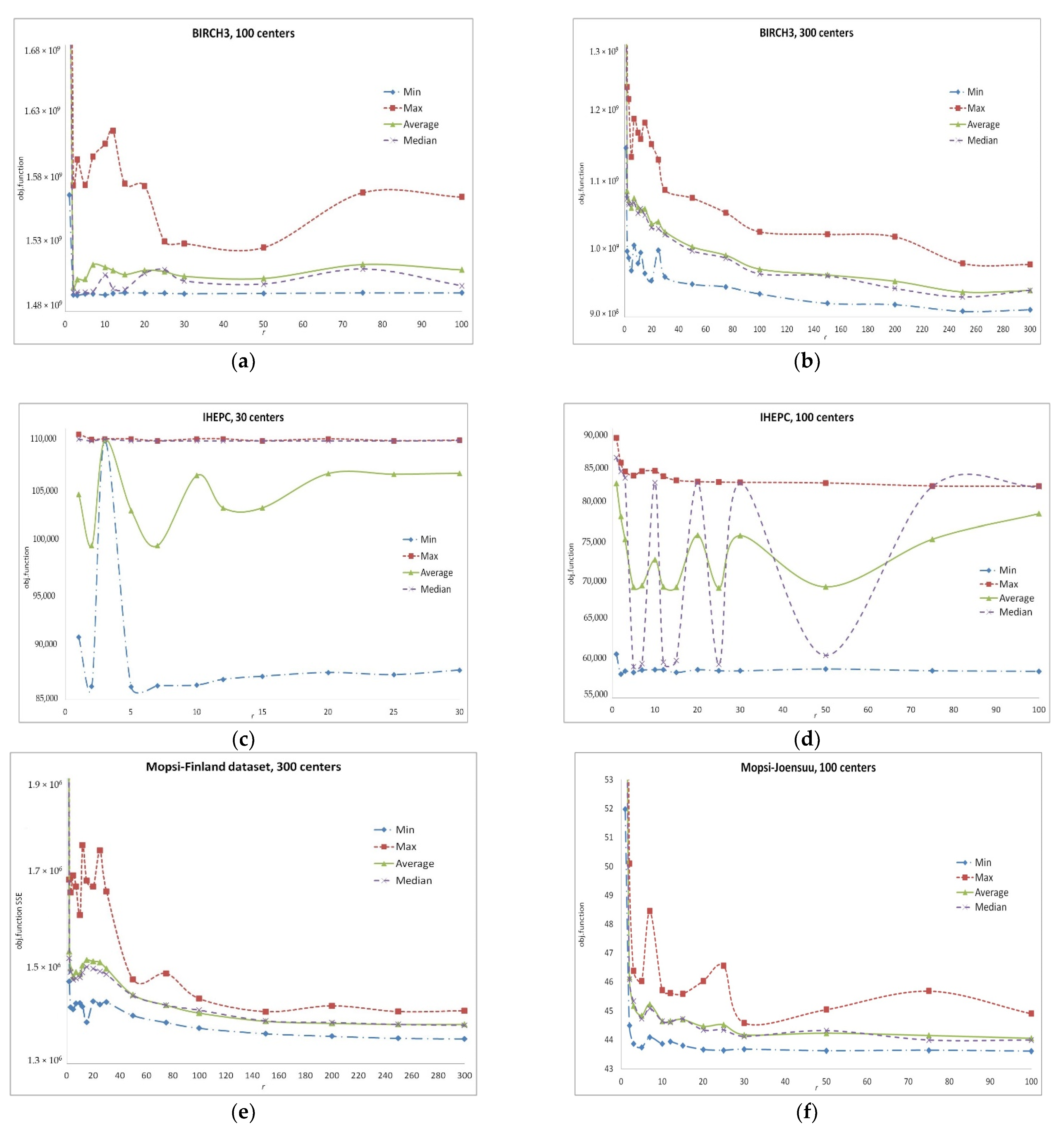
In our computational experiments (described in detail in Section 3) on various problems from repositories [94,95], we investigated the dependence of the efficiency (ability to reach the minimum values of the objective functions) of the search in SWAPr neighborhood on the parameter r. The results obtained after the fixed runtime are given in Figure 1. Obviously, these results are highly dependent on r.
2.2. Greedy Agglomerative Procedures
The agglomerative approach to solving the p-median problem is often successful [70]. To solve the p-median problem in a continuous space, the authors of [60] use genetic algorithms with various crossover operators based on greedy agglomerative procedures. Alp, Erkut, and Drezner in [70] presented a genetic algorithm for facility location problems, where evolution is facilitated by a greedy agglomerative heuristic procedure. A genetic algorithm with a faster greedy heuristic procedure for clustering and location problems was also proposed in [71].
Greedy agglomerative procedures can be used as independent algorithms or embedded in VNS or evolutionary algorithms [52,96]. Such procedures can be described as follows in Algorithm 2:
| Algorithm 2 BasicAggl (S) |
| Require: Set of initial centroids S = {X1, …, XK}, |S| = K > k, required final number of centroids k. |
| Improve S with the two-step local search algorithm if possible; |
| while |S| > k do |
| for do |
| end for; |
| Select a subset S’⊂S of to remove centroids with the minimum values of the corresponding variables Fi; // By default, rtoremove = 1; |
| Improve this new solution with the two-step local search algorithm; |
| end while. |
To improve the performance of such a procedure, the number of simultaneously eliminated centers can be calculated as . In [52,97], the authors used the elimination coefficient value = 0.2. This means that at each iteration, up to 20% of the excessive centers are eliminated, and such values are proved to make the algorithm faster.
The agglomerative procedure for obtaining an AGGLr neighborhood can be defined as follows in Algorithm 3:
| Algorithm 3 AGGLr (S, S2) |
| Require: Two sets of centers S, S2, |S|=|S2|= p, the number of centers r of the solution S2 which are used to obtain the resulting solution, . |
| for do |
| 1. Select a subset ; |
| 2. |
| 3. if F(S’) < F(S) then |
| end if; |
| end for; |
| return S. |
Such procedures use various values of , and nrepeats depends on r: nrepeats = max {1,}.
If the solution S2 is fixed, then all possible results of applying the AGGLr(S, S2) procedure form a neighborhood of the solution S, and S2 as well as r are parameters of such a neighborhood. If S2 is a randomly chosen locally optimal solution obtained by ALA (S2′) procedure applied to a randomly chosen subset , then we deal with a randomized neighborhood.
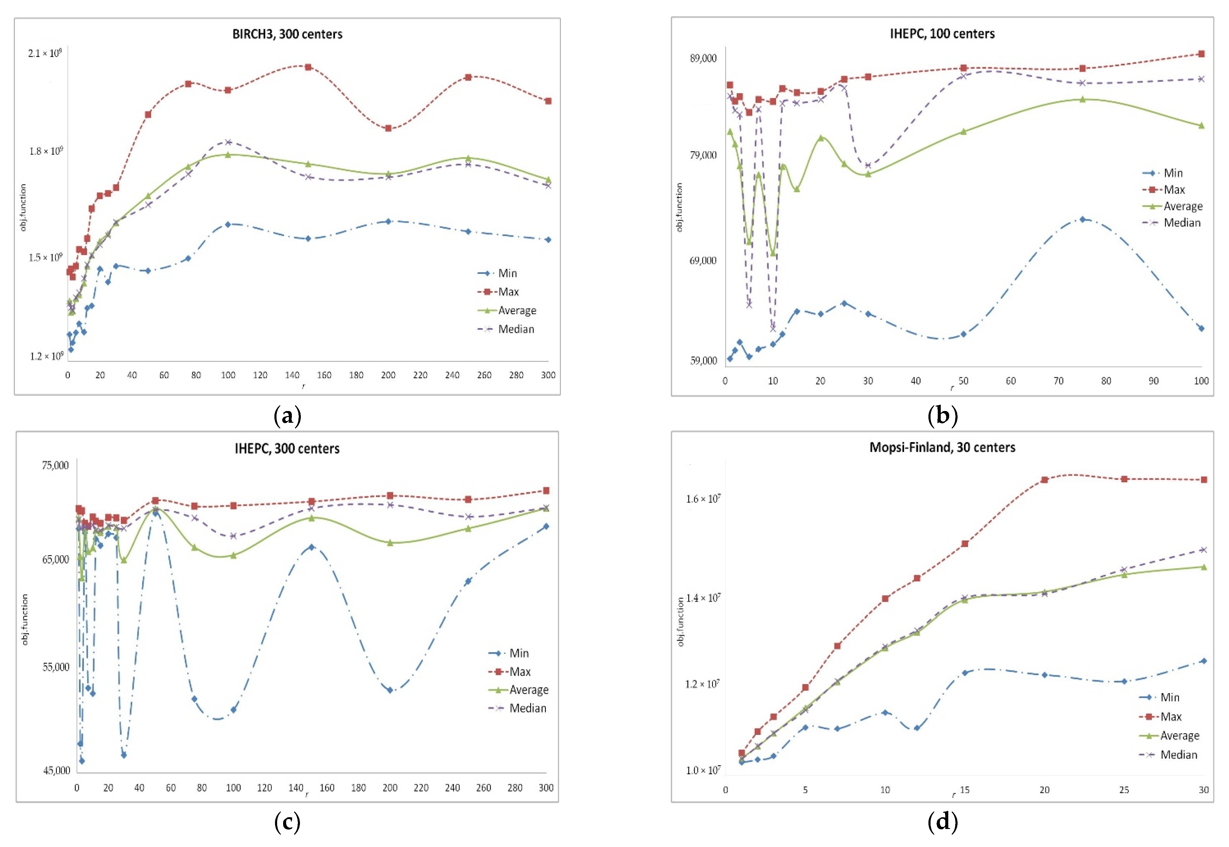
Let us denote such a neighborhood by AGGLr (S). Our experiments demonstrate that the obtained result of the local search in AGGLr neighborhoods strongly depends on r (see Figure 2).
As mentioned above, the greedy agglomerative procedure AGGLr can be used as the crossover operator of the genetic algorithms. Algorithms proposed in [52,71] use such procedures with r = 1 and r = p for solving the k-means and p-median problems.
As a rule, the VNS algorithms move from neighborhoods of lower cardinality to wider neighborhoods. For instance, in [52], the authors propose a sequential search in the neighborhoods AGGL1AGGLrandomAGGLpAGGL1… Here, AGGLrandom is a neighborhood with randomly selected . In this case, the initial neighborhood type has a strong influence on the result [52]. Figure 1 shows that the dependence of the obtained objective function value on r is complex. For the specific problems, there may exist specific values of the parameter r which enable us to obtain better results which are hardly predictable. Nevertheless, a search algorithm may collect the information of the most efficient values of r during its runtime.
2.3. CUDA Implementation of Greedy Agglomerative Procedures
Compute Unified Device Architecture (CUDA) is a hardware-software parallel computing architecture that can significantly increase computational performance [98] designed for the effective use of non-graphical computing on the graphics processing units (GPUs). A GPU is a set of multiprocessors that simultaneously execute parallel threads grouped into data blocks. The threads execute the same instructions on different data in parallel. Communication and synchronization in blocks is impossible.
A thread is assigned an identifier (threadIdx.x) depending on its position in the block, and a block identifier (blockIdx.x) is also assigned to a thread depending on its position in the grid. The thread and block identifiers are available at run time, which allows us to set specific memory access patterns. Each thread in the GPU performs the same procedure, known as the kernel [98].
CUDA versions of the algorithms for solving discrete p-median problems [99,100,101] (which actually solve rather small discrete problems from the OR (Operation Research) Library) as well as parallel implementations of the ALA algorithm for the k-means problems are described in the modern literature [74,98,102]. In our research, we take into account the specificity of the continuous problems.
For large amounts of data, calculating the distances from demand points to cluster centers is the most computationally expensive part of the ALA algorithm. The distances should be calculated to all centers, since the algorithm does not know in advance which center is the nearest one. Traditionally used in solving the k-means problem, this approach can be accelerated by using the triangle inequality [103,104] in the case of p-median problems: if the displacement of the th center relative to the previous iteration was , and its distance to the th demand point was , then the new distance lies within . If :
such that for new distances, . Knowing all distances from the previous iteration and the shift of the centers , we can avoid calculating a significant part of the distances at each iteration, which is especially important when processing multidimensional data. Nevertheless, for large-scale problems, matrix requires a significant additional amount of memory ( values). Moreover, checking the condition (7) for each pair which requires significantly less computational resources than distance calculation
will not accelerate the execution of the algorithm in the case of its CUDA implementation, which assumes strictly simultaneous execution of all instructions by all threads. Therefore, in this work, we do not use of the triangle inequality to accelerate the CUDA version of the ALA algorithm, although more complex implementations for CUDA could probably take advantage of the triangle inequality.
Note that the distances (8) are calculated both in Step 1 of Algorithm 1, and in its Step 2 which includes the iteration of the Weiszfeld procedure (4).
We used the following CUDA implementation of Step 1 of Algorithm 1. The step is divided into two parts. First, variables common for all threads are initialized Algorithm 4:
| Algorithm 4 CUDA implementation of Step 1 in the ALA algorithm, part 1 (initialization) |
| // Here, are vectors used for recalculation of centers. |
| // Counters of objects assigned to each of centers. |
| // are used to calculate . |
| // -dimensional vectors to calculate . |
For the rest of the CUDA implementation of Step 1 of the ALA algorithm, we used the number of threads for each CUDA block. The number of blocks is calculated as
Thus, each thread processes a single demand point in Algorithm 5:
| Algorithm 5 CUDA implementation of Step 1 in the ALA algorithm |
| ifthen |
| return |
| end if |
| // number of a center for the th data point |
| ; // Assign to center . |
| ; ; ; ; |
| Synchronize threads. |
The parallel implementation of Step 2 of the ALA algorithm (see Algorithm 6) uses threads for each CUDA block. The number of blocks is . The variable, common to all threads, is initialized to 0.
| Algorithm 6 CUDA implementation of Step 2 in the ALA algorithm |
| ifthen |
| return; |
| end if; |
| ; |
| ifthen |
| ; |
| end if; |
| ; |
| Synchronize threads. |
Variable is used at the last step of the ALA algorithm and signals the need to continue the iterations.
In addition, we implemented Step 3 of BasicAggl algorithm on the GPU. At this step, Algorithm 2 calculates the sum of the distances after removing a single center with index : . Knowing the objective function value for set of centers, we can calculate its new value
where
Here, Ci’ is the center number which Ai’ is assigned to (nearest to Xi’). We also used 512 threads per block, the number of blocks is calculated according to (9).
After initialization of common variable Dsum←0, the Algorithm 7 is started in a separate thread for each data point:
| Algorithm 7 CUDA implementation of Step 3 in Algorithm 2 |
| ; |
| ifthen |
| return; |
| end if; |
| Calculate in accordance with (2.8); |
| ifthen |
| ; |
| end if; |
| Synchronize threads. |
After parallel running this algorithm, is calculated in accordance with (10) on Step 3 of Algorithm 2: .
The remaining parts of our GA are implemented by the central processor unit. The remaining parts performing the selection do not have any significant effect on the calculation speed. This CUDA implementation of the ALA algorithm enables us to use both the ALA algorithm and more complex algorithms that include it, on large amounts of data, up to millions of demand points.
2.4. New Algorithm
As in local search algorithms, in accordance with the general idea of (1 + 1)-EAs, our new algorithm successively improves the single intermediate solution. To improve it, the AGGLr procedure is applied to it (see Algorithm 3) with an additional intermediate solution randomly generated as the second parameter S2, which is improved by the ALA procedure. A similar idea was applied for the k-means problem in VNS algorithms with randomized neighborhoods [54], which we included in the list of algorithms for comparison. The key feature of the new algorithm is that it does not fix values of the r parameter nor does it generate r values with equal probability, but it adjusts the values of the generation probabilities for each of the possible r values in accordance with the results obtained. If the use of the AGGLr—procedure has resulted in an improvement in the value of the objective function, our algorithm increases the probability Pr for the used r and for values close to it.
The new algorithm can be described as follows in Algorithm 8.
| Algorithm 8 Aggl-EA () |
| Randomly select a subset S {A1, …, AN}; ; assign ; |
| repeat |
| randomly select a subset S2 {A1, …, AN}; ; |
| in proportion to the values of the probabilities Pi, , choose the value of r ; |
| if then |
| ; // we used k1 = 1.1 and k2 = 1.5. |
| // probability normalization |
| S |
| end if; |
| until time limitation is reached. |
| returnS. |
3. Results of Computational Experiments
In all our experiments, we used the classic datasets from the UCI Machine Learning and Clustering basic benchmark repositories [94,95,105]: (a) Individual Household Electric Power Consumption (IHEPC)—energy consumption data of households during several years, more than 2 million demand points (data vectors) in , 0–1 normalized data, “date” and ”time” columns removed; (b) BIRCH3: 100 groups of points of random size, 100,000 demand points in ; (c,d) S1 and S4 datasets, respectively: Gaussian clusters with cluster overlap (5000 demand points in ); (e) Mopsi-Joensuu: geographic locations of users (6014 data vectors, 2 dimensions) in Joensuu city; (f) Mopsi-Finland: geographic locations of users (13,467 data vectors, 2 dimensions) in Finland.
For our computational experiments, we used the following test system: Intel Core 2 Duo E8400 CPU, 16GB RAM, NVIDIA GeForce GTX1050ti GPU with 4096 MB RAM, floating-point performance 2138 GFLOPS. This choice of the GPU hardware was made due to its prevalence, and also one of the best values of the price/performance ratio. The program code was written in C++. We used Visual C++ 2017 compiler embedded into Visual Studio v.15.9.5, NVIDIA CUDA 10.0 Wizards, and NVIDIA Nsight Visual Studio Edition CUDA Support v.6.0.0. For all datasets, 30 attempts were made to run each of algorithms (Algorithms 1–6).
We examined the following algorithms: (a) Lloyd: the ALA algorithm in the multi-start mode; (b) j-means: j-means algorithm (regular search in SWAP1 neighborhood in combination with the ALA algorithm) in the multi-start mode; (c) AGGLr: randomized search in the AGGLr neighborhood, ; (d) SWAPr: local search in SWAPr neighborhoods, (only the best result for is given); (e–g) GH-VNS1, GH-VNS2, GH-VNS3: Variable Neighborhood Search algorithms with neighborhoods formed by application of AGGLr() procedure, see [52]; (h) GA-1POINT: genetic algorithm with a standard 1-point crossover; (i) GA-UNIFORM: genetic algorithm with a standard 1-point crossover and uniform random mutation [56]; (j) Aggl-EA: our new algorithm.
For all datasets, 30 attempts were made to run each of the algorithms (see Table 1 and Table A1, Table A2, Table A3, Table A4, Table A5, Table A6, Table A7, Table A8, Table A9, Table A10, Table A11, Table A12, Table A13, Table A14 and Table A15 in Appendix A). In Table 1, we present the results of our new algorithm Aggl-EA() and the best of listed known algorithms, i.e., known algorithms which provided the best average or median values of the objective function (1) after 30 runs.
For the smallest and simplest test problems (see Table A1 and Table A4 in Appendix A), several algorithms including Aggl-EA() and search in the AGGL neighborhoods resulted in the same objective function value (standard deviation of the result is 0.0) which is probably the global minimum. Nevertheless, the Aggl-EA() algorithm outperforms both genetic algorithms and simplest local search algorithms such as Lloyd() or j-means which do not reach this minimum value in all attempts. For more complex test problems, the comparative efficiency varies. However, there were no test problems for which our new algorithm demonstrated a statistically significant disadvantage in comparison with the best of known algorithms.
The best (minimum), worst (maximum), average, and median values of the achieved objective function were averaged after 30 runs of each algorithm with fixed time limitation. The best average and median values of the objective Function (1) are underlined. We compared our new Aggl-EA () algorithm with known examined algorithm having the best median or average results. The significance of advantage/disadvantage of Aggl-EA() algorithm was estimated with the t-test [106,107] and non-parametric Wilcoxon rank sum test [108,109].
In the analysis of algorithm efficiency, the researchers often estimate the computational expenses as the number of the objective function calculations. The ALA procedure is the most computationally expensive part of all examined algorithms. In the ALA algorithm, the objective Function (1) is never calculated directly. The program code profiling results show that Step 2 of Algorithm 1 and Step 3 of Algorithm 2 occupy more than 99% of computational resources (processor time). These steps were implemented on GPUs. Moreover, we use the same implementation of the ALA procedure and BasicAggl() algorithm for all examined algorithms. Thus, the consumed time could be proportional with the number of iterations of the ALA algorithm (its Step 2) and the most time-consuming iterations of Algorithm 2 (its Step 3). However, the time consumption of these iterations depends on the number of centers which successively decreases during the work of the BasicAggl () algorithm. Thus, for the p-median problems, we used the astronomical time as the most informative unit for the computational expenses.
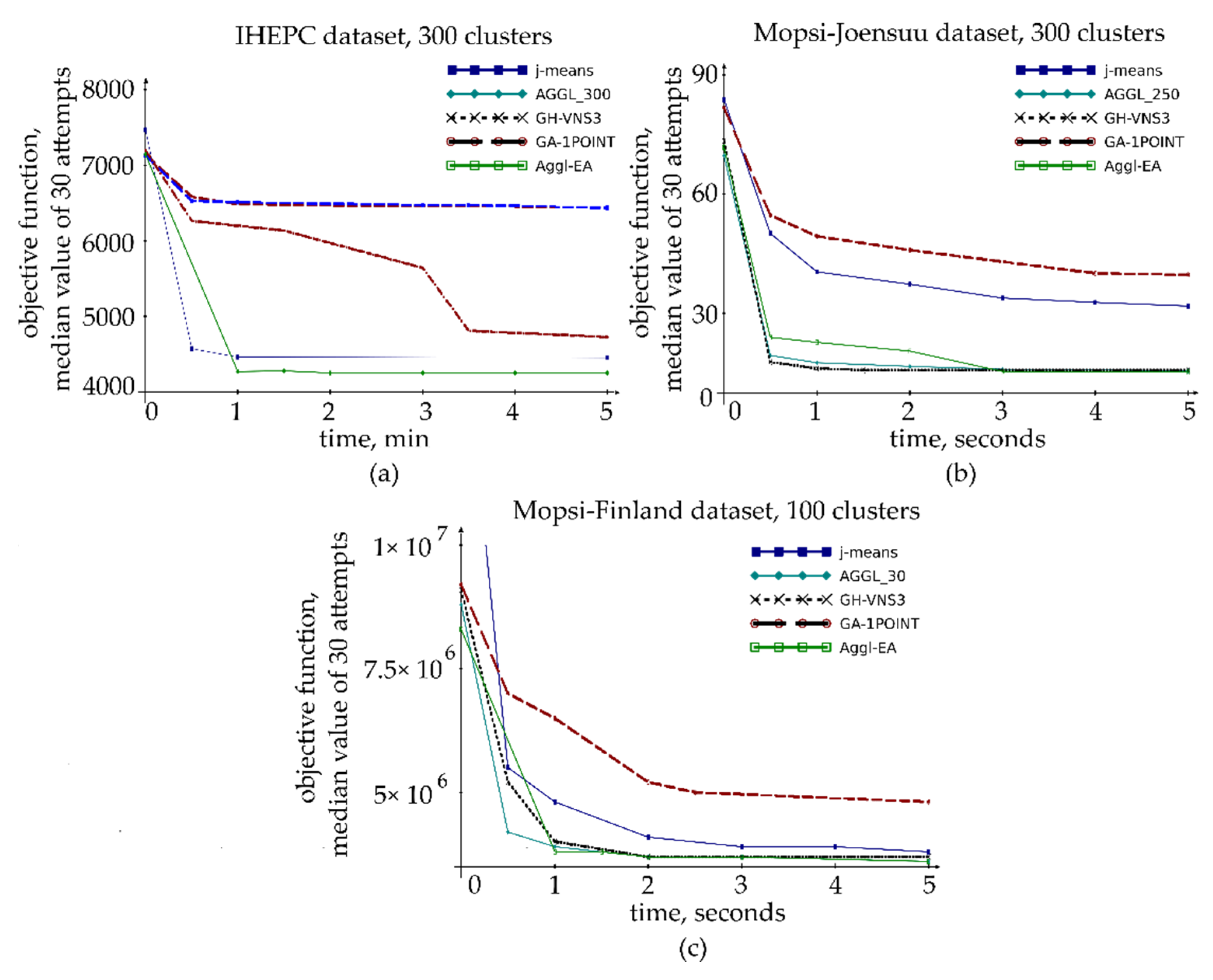
The time limitation plays an important role: the fastest algorithms may stop their convergence after several iterations and, vice versa, the slowest algorithms may continue their slow convergence and outperform the fastest algorithms if we enlarge their time limits. However, our new algorithms demonstrate their comparative advantage within wide time intervals (see Figure 3).
4. Discussion
The genetic algorithms and Variable Neighborhood Search are algorithmic frameworks useful for creating efficient solvers of various problems including location problems such as p-median. The greedy agglomerative approach can be efficiently used as the crossover genetic operator [58,70,71,102] as well as in the VNS [52]. However, as our experiments show (Appendix A), the correct choice of parameter r in such procedures plays the most important role and simple search algorithms with constant value of r may outperform more complex VNS algorithms if r is tuned correctly.
Unlike the majority of evolutionary algorithms, the (1 + 1)-evolutionary algorithms as well as local search algorithms focus on the successive improvement of a single intermediate solution. Successful application of various local search algorithms such as SWAP search, j-means or various VNS algorithms including to the p-median problem shows that the correct choice of a neighborhood or an algorithmic procedure for the successive improvement of a single current solution can be a more profitable strategy for solving practical problems than operating with a large population of solutions. In this work, we have increased the efficiency of one of these procedures by adjusting its parameter. Nevertheless, adjusting the parameters of greedy agglomerative procedures can also enhance the capabilities of genetic algorithms with a greedy agglomerative crossing operator, which, in our opinion, is an urgent area of further research. In addition, similar algorithms can be developed for a wider range of problems, including k-means, k-medoid, and the problem of separating a mixture of probability distributions.
Our new algorithm demands significant computational resources. Nevertheless, obtaining the most accurate results for solving problems, in addition to being of immediate practical importance in the case of a high cost of error, solves the problem of obtaining reference solutions with which the results of other, less computationally expensive algorithms can be compared.
As in the case of the k-means problem [74], the most complex dependence of the greedy procedure efficiency on its parameter r and important advantage of our new algorithm is detected for the largest tested problems (IHEPC dataset) as well as for the problems of “geographic” location (Mopsi datasets) with the sets of demand points formed under the influence of natural factors, as well as factors associated with the development of urban infrastructure.
For the majority of test problems, our computational experiments demonstrate the advantage of our new algorithm or its approximately equal effectiveness in comparison with known algorithms. For large-scale problem, the effect of our new algorithm is more significant. Nevertheless, even with equal results in comparison with known algorithms, our new Aggl-EA algorithm is a more versatile tool due to its ability of adjusting its parameter in accordance with its behavior. Sometimes, our new algorithm demonstrates less stable results (higher standard deviation of the objective function) which may limit its scope or demands running in multi-start mode. Thus, further study of the causes and factors leading to the instability of the result is required.
We considered the use of the self-adjusted agglomerative procedures as the mutation operator of the simplest evolutionary algorithm with no true population of solutions. The efficiency of embedding similar mutation operators (without any self-adjustment) was shown in the paper [96]. Thus, the investigation of the self-adjustment features of other evolutionary operators (first of all, crossover operator of genetic algorithms) is a promising direction for the further research.
5. Conclusions
In this article, we introduced the concept of the AGGLr neighborhood based on the application of the agglomerative procedure, and investigate the search efficiency in such a neighborhood depending on the parameter r. Using the similarities between local search algorithms and (1 + 1)-evolutionary algorithms, as well as the ability of the latter to adapt their search parameters, we introduced our new Aggl-EA () algorithm with an embedded greedy agglomerative procedure with the automatically tuned parameter r. Our computational experiments on large-scale and medium-scale problems demonstrate the advantages of the new algorithm in comparison with known algorithms including the algorithms based on greedy agglomerative procedures.
Our computational experiments confirmed the proposed working hypotheses and led to the following conclusions:
The agglomerative mutation operator, when used as part of an evolutionary algorithm, is not only able to improve its solutions, moreover, it can also be efficiently used as the only evolutionary operator in the (1 + 1)-evolutionary algorithm with results outperforming more complex genetic algorithms. Therefore, self-adjustment capability of other evolutionary operators based on agglomerative procedures is a promising direction for the further research.
The algorithm with the adjustment of the parameter r (the number of excess centers to be removed) of the agglomerative procedure shows the most impressive results in the case of solving large problems, as well as problems of a “geographic” nature, where many points of demand have a complex structure, formed under the influence of natural factors.
Such algorithms, implemented for massively parallel systems, despite the high computational complexity of the embedded agglomerative procedure, ALA-algorithm and Weiszfeld procedure, are capable of solving problems with several million demand points in a reasonable time.
Author Contributions
Conceptualization, L.K.; methodology, L.K. and I.R.; software, L.K.; validation, I.R.; formal analysis, L.K. and G.S.; investigation, I.R.; resources, L.K.; data curation, I.R.; writing—original draft preparation, L.K. and G.S.; writing—review and editing, L.K.; visualization, I.R.; supervision, L.K.; project administration, L.K.; funding acquisition, L.K. All authors have read and agreed to the published version of the manuscript.
Funding
This research was funded by The Ministry of Science and Higher Education of the Russian Federation, project No. FEFE-2020-0013.
Institutional Review Board Statement
Not applicable.
Informed Consent Statement
Not applicable.
Data Availability Statement
Publicly available datasets were analyzed in this study. This data can be found here: http://cs.joensuu.fi/sipu/datasets/ (accessed on 21 April 2020), https://archive.ics.uci.edu/ml/index.php (accessed on 21 April 2020).
Conflicts of Interest
The authors declare no conflict of interest. The funder had no role in the design of the study; in the collection, analyses, or interpretation of data; in the writing of the manuscript, or in the decision to publish the results.
Appendix A. Detailed Results of Computational Experiments

Table A1.
Comparative results for BIRCH3 dataset. 105 data vectors in , p = 30 centers, time limitation 10 s.
Table A1.
Comparative results for BIRCH3 dataset. 105 data vectors in , p = 30 centers, time limitation 10 s.
| Algorithm or Neighborhood | Achieved Objective Function Values (1) Summarized after 30 Runs | ||||
|---|---|---|---|---|---|
| Min (Record) | Max (Worst) | Average | Median | Std. Dev | |
| Lloyd (multistart) | 4.38183 × 10⁹ | 4.67540 × 10⁹ | 4.52387 × 10⁹ | 4.51929 × 10⁹ | 7.82433 × 10⁷ |
| j-means (SWAP1 + Lloyd) | 3.56107 × 10⁹ | 5.25877 × 10⁹ | 3.92248 × 10⁹ | 3.88872 × 10⁹ | 3.09203 × 10⁸ |
| AGGL1 | 3.45692 × 10⁹ | 3.56599 × 10⁹ | 3.46697 × 10⁹ | 3.45692 × 10⁹ | 2.40890 × 10⁷ |
| AGGL2 | 3.45057 × 10⁹ | 3.45692 × 10⁹ | 3.45650 × 10⁹ | 3.45692 × 10⁹ | 1.61204 × 10⁶ |
| AGGL3 | 3.45057 × 10⁹ | 3.45692 × 10⁹ | 3.45650 × 10⁹ | 3.45692 × 10⁹ | 1.61204 × 10⁶ |
| AGGL5–20 (equal results) | 3.45692 × 10⁹ | 3.45692 × 10⁹ | 3.45692 × 10⁹ | 3.45692 × 10⁹ | 0.00000 |
| AGGL25 | 3.45057 × 10⁹ | 3.45057 × 10⁹ | 3.45057 × 10⁹ | 3.45057 × 10⁹ | 46.7390 |
| AGGL30 | 3.45057 × 10⁹ | 3.45057 × 10⁹ | 3.45057 × 10⁹ | 3.45057 × 10⁹ | 127.558 |
| GH-VNS1-3 (equal results) | 3.45057 × 10⁹ | 3.45057 × 10⁹ | 3.45057 × 10⁹ | 3.45057 × 10⁹ | 0.00000 |
| SWAP1 (the best of SWAP) | 3.70386 × 10⁹ | 4.43612 × 10⁹ | 3.89665 × 10⁹ | 3.89201 × 10⁹ | 1.24246 × 10⁸ |
| GA-1POINT | 3.51505 × 10⁹ | 3.63646 × 10⁹ | 3.56546 × 10⁹ | 3.56848 × 10⁹ | 3.24395 × 10⁷ |
| GA-UNIFORM | 3.45057 × 10⁹ | 3.59155 × 10⁹ | 3.49515 × 10⁹ | 3.49778 × 10⁹ | 3.07081 × 10⁷ |
| Aggl-EA | 3.45057 × 10⁹ | 3.45057 × 10⁹ | 3.45057 × 10⁹ | 3.45057 × 10⁹ | 0.00000 |
Note (for all tables): the best results are underlined.
Table A2.
Comparative results for BIRCH3 dataset. 105 data vectors in , p = 100 centers, time limitation 10 s.
Table A2.
Comparative results for BIRCH3 dataset. 105 data vectors in , p = 100 centers, time limitation 10 s.
| Algorithm or Neighborhood | Achieved Objective Function Values (1) Summarized after 30 Runs | ||||
|---|---|---|---|---|---|
| Min (Record) | Max (Worst) | Average | Median | Std. Dev | |
| Lloyd (multistart) | 2.27163 × 10⁹ | 2.54224 × 10⁹ | 2.44280 × 10⁹ | 2.46163 × 10⁹ | 7.42330 × 10⁷ |
| j-means (SWAP1 + Lloyd) | 1.52130 × 10⁹ | 1.88212 × 10⁹ | 1.69226 × 10⁹ | 1.67712 × 10⁹ | 8.03684 × 10⁷ |
| AGGL1 | 1.56737 × 10⁹ | 2.14554 × 10⁹ | 1.81181 × 10⁹ | 1.80137 × 10⁹ | 1.60897 × 10⁸ |
| AGGL2 | 1.49271 × 10⁹ | 1.57474 × 10⁹ | 1.49822 × 10⁹ | 1.49445 × 10⁹ | 1.51721 × 10⁷ |
| AGGL3 | 1.49232 × 10⁹ | 1.59406 × 10⁹ | 1.50429 × 10⁹ | 1.49447 × 10⁹ | 2.64626 × 10⁷ |
| AGGL5 | 1.49341 × 10⁹ | 1.57503 × 10⁹ | 1.50433 × 10⁹ | 1.49439 × 10⁹ | 2.44200 × 10⁷ |
| AGGL7 | 1.49341 × 10⁹ | 1.59630 × 10⁹ | 1.51531 × 10⁹ | 1.49515 × 10⁹ | 3.58332 × 10⁷ |
| AGGL10 | 1.49261 × 10⁹ | 1.60585 × 10⁹ | 1.51345 × 10⁹ | 1.50733 × 10⁹ | 2.79785 × 10⁷ |
| AGGL12 | 1.49358 × 10⁹ | 1.61554 × 10⁹ | 1.51105 × 10⁹ | 1.49754 × 10⁹ | 3.16092 × 10⁷ |
| AGGL15 | 1.49414 × 10⁹ | 1.57599 × 10⁹ | 1.50791 × 10⁹ | 1.49667 × 10⁹ | 2.39108 × 10⁷ |
| AGGL20 | 1.49406 × 10⁹ | 1.57432 × 10⁹ | 1.51096 × 10⁹ | 1.50880 × 10⁹ | 1.83795 × 10⁷ |
| AGGL25 | 1.49386 × 10⁹ | 1.53280 × 10⁹ | 1.51017 × 10⁹ | 1.51159 × 10⁹ | 1.23389 × 10⁷ |
| AGGL30 | 1.49355 × 10⁹ | 1.53113 × 10⁹ | 1.50656 × 10⁹ | 1.50311 × 10⁹ | 1.12716 × 10⁷ |
| AGGL50 | 1.49380 × 10⁹ | 1.52818 × 10⁹ | 1.50495 × 10⁹ | 1.50073 × 10⁹ | 1.11666 × 10⁷ |
| AGGL75 | 1.49415 × 10⁹ | 1.56935 × 10⁹ | 1.51541 × 10⁹ | 1.51203 × 10⁹ | 1.95288 × 10⁷ |
| AGGL100 | 1.49413 × 10⁹ | 1.56603 × 10⁹ | 1.51133 × 10⁹ | 1.49943 × 10⁹ | 2.01570 × 10⁷ |
| GH-VNS1 | 1.49362 × 10⁹ | 1.66273 × 10⁹ | 1.54540 × 10⁹ | 1.51469 × 10⁹ | 5.07461 × 10⁷ |
| GH-VNS2 | 1.49413 × 10⁹ | 1.59073 × 10⁹ | 1.50692 × 10⁹ | 1.50235 × 10⁹ | 1.87495 × 10⁷ |
| GH-VNS3 | 1.49247 × 10⁹ | 1.55423 × 10⁹ | 1.50561 × 10⁹ | 1.49497 × 10⁹ | 1.84421 × 10⁷ |
| SWAP1 (the best of SWAP) | 1.70412 × 10⁹ | 2.00689 × 10⁹ | 1.83218 × 10⁹ | 1.83832 × 10⁹ | 6.04418 × 10⁷ |
| GA-1POINT | 1.61068 × 10⁹ | 1.85786 × 10⁹ | 1.69042 × 10⁹ | 1.65346 × 10⁹ | 7.23930 × 10⁷ |
| GA-UNIFORM | 1.67990 × 10⁹ | 1.92521 × 10⁹ | 1.77471 × 10⁹ | 1.76783 × 10⁹ | 6.95451 × 10⁷ |
| Aggl-EA | 1.49199 × 10⁹ | 1.57449 × 10⁹ | 1.50670 × 10⁹ | 1.49495 × 10⁹ | 2.46374 × 10⁷ |
Table A3.
Comparative results for BIRCH3 dataset. 105 data vectors in , p = 300 centers, time limitation 10 s.
Table A3.
Comparative results for BIRCH3 dataset. 105 data vectors in , p = 300 centers, time limitation 10 s.
| Algorithm or Neighborhood | Achieved Objective Function Values (1) Summarized after 30 Runs | ||||
|---|---|---|---|---|---|
| Min (Record) | Max (Worst) | Average | Median | Std. Dev | |
| Lloyd (multistart) | 1.54171 × 10⁹ | 1.64834 × 10⁹ | 1.59859 × 10⁹ | 1.60045 × 10⁹ | 2.62443 × 10⁷ |
| j-means (SWAP1 + Lloyd) | 9.95926 × 10⁸ | 1.15171 × 10⁹ | 1.05927 × 10⁹ | 1.04561 × 10⁹ | 4.63788 × 10⁷ |
| AGGL1 | 1.14784 × 10⁹ | 1.88404 × 10⁹ | 1.47311 × 10⁹ | 1.42352 × 10⁹ | 1.94210 × 10⁸ |
| AGGL2 | 9.96893 × 10⁸ | 1.23746 × 10⁹ | 1.08456 × 10⁹ | 1.07354 × 10⁹ | 5.76487 × 10⁷ |
| AGGL3 | 9.87064 × 10⁸ | 1.21980 × 10⁹ | 1.07148 × 10⁹ | 1.06503 × 10⁹ | 4.84664 × 10⁷ |
| AGGL5 | 9.68357 × 10⁸ | 1.13508 × 10⁹ | 1.06002 × 10⁹ | 1.06617 × 10⁹ | 4.50726 × 10⁷ |
| AGGL7 | 1.00537 × 10⁹ | 1.19050 × 10⁹ | 1.07440 × 10⁹ | 1.06799 × 10⁹ | 4.73520 × 10⁷ |
| AGGL10 | 9.78925 × 10⁸ | 1.17041 × 10⁹ | 1.06123 × 10⁹ | 1.05264 × 10⁹ | 5.10834 × 10⁷ |
| AGGL12 | 9.94720 × 10⁸ | 1.16133 × 10⁹ | 1.05659 × 10⁹ | 1.05930 × 10⁹ | 3.59604 × 10⁷ |
| AGGL15 | 9.64129 × 10⁸ | 1.18512 × 10⁹ | 1.05884 × 10⁹ | 1.04935 × 10⁹ | 5.54774 × 10⁷ |
| AGGL20 | 9.53544 × 10⁸ | 1.15383 × 10⁹ | 1.03729 × 10⁹ | 1.03124 × 10⁹ | 4.58983 × 10⁷ |
| AGGL25 | 9.98103 × 10⁸ | 1.13062 × 10⁹ | 1.03990 × 10⁹ | 1.02958 × 10⁹ | 3.39141 × 10⁷ |
| AGGL30 | 9.59132 × 10⁸ | 1.08646 × 10⁹ | 1.02528 × 10⁹ | 1.02102 × 10⁹ | 3.48713 × 10⁷ |
| AGGL50 | 9.48152 × 10⁸ | 1.07480 × 10⁹ | 1.00313 × 10⁹ | 9.97259 × 10⁸ | 2.65919 × 10⁷ |
| AGGL75 | 9.44390 × 10⁸ | 1.05320 × 10⁹ | 9.90754 × 10⁸ | 9.86511 × 10⁸ | 3.04626 × 10⁷ |
| AGGL100 | 9.33977 × 10⁸ | 1.02524 × 10⁹ | 9.70365 × 10⁸ | 9.63525 × 10⁸ | 2.48207 × 10⁷ |
| AGGL150 | 9.20206 × 10⁸ | 1.02162 × 10⁹ | 9.61877 × 10⁸ | 9.60465 × 10⁸ | 2.42984 × 10⁷ |
| AGGL200 | 9.18310 × 10⁸ | 1.01805 × 10⁹ | 9.52666 × 10⁸ | 9.42071 × 10⁸ | 2.73422 × 10⁷ |
| AGGL250 | 9.08532 × 10⁸ | 9.78792 × 10⁸ | 9.36947 × 10⁸ | 9.29497 × 10⁸ | 1.97893 × 10⁷ |
| AGGL300 | 9.10975 × 10⁸ | 9.77193 × 10⁸ | 9.39030 × 10⁸ | 9.39434 × 10⁸ | 1.27907 × 10⁷ |
| GH-VNS1 | 1.00289 × 10⁹ | 1.08471 × 10⁹ | 1.03856 × 10⁹ | 1.03485 × 10⁹ | 2.20294 × 10⁷ |
| GH-VNS2 | 9.68045 × 10⁸ | 1.11832 × 10⁹ | 1.01461 × 10⁹ | 1.00404 × 10⁹ | 3.80607 × 10⁷ |
| GH-VNS3 | 9.12455 × 10⁸ | 9.44414 × 10⁸ | 9.31225 × 10⁸ | 9.32001 × 10⁸ | 8.25653 × 10⁶ |
| SWAP2 (the best of SWAP by avg.) | 1.23379 × 10⁹ | 1.46395 × 10⁹ | 1.33987 × 10⁹ | 1.35305 × 10⁹ | 5.64094 × 10⁷ |
| SWAP3 (the best of SWAP by median) | 1.25432 × 10⁹ | 1.44136 × 10⁹ | 1.34388 × 10⁹ | 1.34424 × 10⁹ | 5.01104 × 10⁷ |
| GA-1POINT | 1.11630 × 10⁹ | 1.38598 × 10⁹ | 1.23404 × 10⁹ | 1.22828 × 10⁹ | 7.05936 × 10⁷ |
| GA-UNIFORM | 1.17534 × 10⁹ | 1.37190 × 10⁹ | 1.26758 × 10⁹ | 1.25424 × 10⁹ | 5.20153 × 10⁷ |
| Aggl-EA | 9.14179 × 10⁸ | 9.71905 × 10⁸ | 9.34535 × 10⁸ | 9.33403 × 10⁸ | 1.51920 × 10⁷ |
Table A4.
Comparative results for S1 dataset. 5000 data vectors in , p = 15 centers, time limitation 1 s.
Table A4.
Comparative results for S1 dataset. 5000 data vectors in , p = 15 centers, time limitation 1 s.
| Algorithm or Neighborhood | Achieved Objective Function Values (1) Summarized after 30 Runs | ||||
|---|---|---|---|---|---|
| Min (Record) | Max (Worst) | Average | Median | Std. Dev | |
| Lloyd (multistart) | 1.69034 × 10⁸ | 2.02847 × 10⁸ | 1.79099 × 10⁸ | 1.69034 × 10⁸ | 1.56374 × 10⁷ |
| j-means (SWAP1 + Lloyd) | 1.69034 × 10⁸ | 2.18797 × 10⁸ | 1.74375 × 10⁸ | 1.69034 × 10⁸ | 1.40223 × 10⁷ |
| AGGL1 | 1.69034 × 10⁸ | 2.02619 × 10⁸ | 1.71265 × 10⁸ | 1.69034 × 10⁸ | 8.49108 × 10⁶ |
| AGGL2-15 (equal results) | 1.69034 × 10⁸ | 1.69034 × 10⁸ | 1.69034 × 10⁸ | 1.69034 × 10⁸ | 0.00000 |
| SWAP1 (the best of SWAP) | 1.69034 × 10⁸ | 2.08453 × 10⁸ | 1.70348 × 10⁸ | 1.69034 × 10⁸ | 7.19690 × 10⁶ |
| GA-1POINT | 1.69034 × 10⁸ | 2.02783 × 10⁸ | 1.76877 × 10⁸ | 1.69034 × 10⁸ | 1.44603 × 10⁷ |
| GA-UNIFORM | 1.69034 × 10⁸ | 1.69034 × 10⁸ | 1.69034 × 10⁸ | 1.69034 × 10⁸ | 2.92119 |
| Aggl-EA | 1.69034 × 10⁸ | 1.69034 × 10⁸ | 1.69034 × 10⁸ | 1.69034 × 10⁸ | 0.00000 |
Table A5.
Comparative results for S1 dataset. 5000 data vectors in , p = 50 centers, time limitation 1 s.
Table A5.
Comparative results for S1 dataset. 5000 data vectors in , p = 50 centers, time limitation 1 s.
| Algorithm or Neighborhood | Achieved Objective Function Values (1) Summarized after 30 Runs | ||||
|---|---|---|---|---|---|
| Min (Record) | Max (Worst) | Average | Median | Std. Dev | |
| Lloyd (multistart) | 1.14205 × 10⁸ | 1.16737 × 10⁸ | 1.15594 × 10⁸ | 1.15666 × 10⁸ | 6.33573 × 10⁵ |
| j-means (SWAP1 + Lloyd) | 1.13500 × 10⁸ | 1.17631 × 10⁸ | 1.15035 × 10⁸ | 1.14954 × 10⁸ | 9.38353 × 10⁵ |
| AGGL1 | 1.13121 × 10⁸ | 1.15265 × 10⁸ | 1.14219 × 10⁸ | 1.14035 × 10⁸ | 6.23645 × 10⁵ |
| AGGL2 | 1.12430 × 10⁸ | 1.12572 × 10⁸ | 1.12475 × 10⁸ | 1.12464 × 10⁸ | 3.76180 × 10⁴ |
| AGGL3 | 1.12426 × 10⁸ | 1.12548 × 10⁸ | 1.12465 × 10⁸ | 1.12457 × 10⁸ | 2.92460 × 10⁴ |
| AGGL5 | 1.12446E × 108 | 1.12552 × 10⁸ | 1.12487 × 10⁸ | 1.12483 × 10⁸ | 3.00588 × 10⁴ |
| AGGL7 | 1.12437 × 10⁸ | 1.12591 × 10⁸ | 1.12481 × 10⁸ | 1.12478 × 10⁸ | 3.26658 × 10⁴ |
| AGGL10 | 1.12462 × 10⁸ | 1.12558 × 10⁸ | 1.12500 × 10⁸ | 1.12500 × 10⁸ | 2.68212 × 10⁴ |
| AGGL15 | 1.12462 × 10⁸ | 1.12579 × 10⁸ | 1.12526 × 10⁸ | 1.12528 × 10⁸ | 2.83854 × 10⁴ |
| AGGL20 | 1.12461 × 10⁸ | 1.12590 × 10⁸ | 1.12535 × 10⁸ | 1.12538 × 10⁸ | 3.27419 × 10⁴ |
| AGGL25 | 1.12472 × 10⁸ | 1.12632 × 10⁸ | 1.12541 × 10⁸ | 1.12543 × 10⁸ | 4.34545 × 10⁴ |
| AGGL30 | 1.12523 × 10⁸ | 1.12662 × 10⁸ | 1.12572 × 10⁸ | 1.12566 × 10⁸ | 3.55121 × 10⁴ |
| AGGL50 | 1.12541 × 10⁸ | 1.12848 × 10⁸ | 1.12666 × 10⁸ | 1.12651 × 10⁸ | 7.48936 × 10⁴ |
| GH-VNS1 | 1.12419 × 10⁸ | 1.12796 × 10⁸ | 1.12467 × 10⁸ | 1.12446 × 10⁸ | 7.47785 × 10⁴ |
| GH-VNS2 | 1.12472 × 10⁸ | 1.12601 × 10⁸ | 1.12525 × 10⁸ | 1.12519 × 10⁸ | 3.37221 × 10⁴ |
| GH-VNS3 | 1.12531 × 10⁸ | 1.12969 × 10⁸ | 1.12712 × 10⁸ | 1.12708 × 10⁸ | 9.60927 × 10⁴ |
| SWAP1 (the best of SWAP) | 1.13142 × 10⁸ | 1.16627 × 10⁸ | 1.14430 × 10⁸ | 1.14412 × 10⁸ | 8.48529 × 10⁵ |
| GA-1POINT | 1.14271 × 10⁸ | 1.16790 × 10⁸ | 1.15443 × 10⁸ | 1.15343 × 10⁸ | 7.16204 × 10⁵ |
| GA-UNIFORM | 1.13119 × 10⁸ | 1.15805 × 10⁸ | 1.14384 × 10⁸ | 1.14405 × 10⁸ | 6.75227 × 10⁵ |
| Aggl-EA | 1.12476 × 10⁸ | 1.15978 × 10⁸ | 1.14049 × 10⁸ | 1.13985 × 10⁸ | 1.05017 × 10⁶ |
Table A6.
Comparative results for S4 dataset. 5000 data vectors in , p = 15 centers, time limitation 1 s.
Table A6.
Comparative results for S4 dataset. 5000 data vectors in , p = 15 centers, time limitation 1 s.
| Algorithm or Neighborhood | Achieved Objective Function Values (1) Summarized after 30 Runs | ||||
|---|---|---|---|---|---|
| Min (Record) | Max (Worst) | Average | Median | Std. Dev | |
| Lloyd (multistart) | 2.27694 × 10⁸ | 2.27694 × 10⁸ | 2.27694 × 10⁸ | 2.27694 × 10⁸ | 25.4490 |
| j-means (SWAP1 + Lloyd) | 2.27694 × 10⁸ | 2.60475 × 10⁸ | 2.30812 × 10⁸ | 2.27694 × 10⁸ | 7.33507 × 10⁶ |
| AGGL1 | 2.27694 × 10⁸ | 2.27694 × 10⁸ | 2.27694 × 10⁸ | 2.27694 × 10⁸ | 26.4692 |
| AGGL2 | 2.27694 × 10⁸ | 2.27694 × 10⁸ | 2.27694 × 10⁸ | 2.27694 × 10⁸ | 6.88293 |
| AGGL3 | 2.27694 × 10⁸ | 2.27694 × 10⁸ | 2.27694 × 10⁸ | 2.27694 × 10⁸ | 7.84212 |
| AGGL5 | 2.27694 × 10⁸ | 2.27694 × 10⁸ | 2.27694 × 10⁸ | 2.27694 × 10⁸ | 14.9936 |
| AGGL7 | 2.27694 × 10⁸ | 2.27694 × 10⁸ | 2.27694 × 10⁸ | 2.27694 × 10⁸ | 26.1335 |
| AGGL10 | 2.27694 × 10⁸ | 2.27694 × 10⁸ | 2.27694 × 10⁸ | 2.27694 × 10⁸ | 112.307 |
| AGGL12 | 2.27694 × 10⁸ | 2.27694 × 10⁸ | 2.27694 × 10⁸ | 2.27694 × 10⁸ | 41.2754 |
| AGGL15 | 2.27694 × 10⁸ | 2.27694 × 10⁸ | 2.27694 × 10⁸ | 2.27694 × 10⁸ | 81.9819 |
| GH-VNS1 | 2.27694 × 10⁸ | 2.27694 × 10⁸ | 2.27694 × 10⁸ | 2.27694 × 10⁸ | 0.00000 |
| GH-VNS2 | 2.27694 × 10⁸ | 2.27694 × 10⁸ | 2.27694 × 10⁸ | 2.27694 × 10⁸ | 35.8018 |
| GH-VNS3 | 2.27694 × 10⁸ | 2.27694 × 10⁸ | 2.27694 × 10⁸ | 2.27694 × 10⁸ | 81.1213 |
| SWAP1 (the best of SWAP) | 2.27694 × 10⁸ | 2.38720 × 10⁸ | 2.28342 × 10⁸ | 2.27694 × 10⁸ | 2.48983 × 10⁶ |
| GA-1POINT | 2.27694 × 10⁸ | 2.27694 × 10⁸ | 2.27694 × 10⁸ | 2.27694 × 10⁸ | 17.3669 |
| GA-UNIFORM | 2.27694 × 10⁸ | 2.27694 × 10⁸ | 2.27694 × 10⁸ | 2.27694 × 10⁸ | 8.55973 |
| Aggl-EA | 2.27694 × 10⁸ | 2.27694 × 10⁸ | 2.27694 × 10⁸ | 2.27694 × 10⁸ | 78.6011 |
Table A7.
Comparative results for S4 dataset. 5000 data vectors in , p = 50 centers, time limitation 1 s.
Table A7.
Comparative results for S4 dataset. 5000 data vectors in , p = 50 centers, time limitation 1 s.
| Algorithm or Neighborhood | Achieved Objective Function Values (1) Summarized after 30 Runs | ||||
|---|---|---|---|---|---|
| Min (Record) | Max (Worst) | Average | Median | Std. Dev | |
| Lloyd (multistart) | 1.35718 × 10⁸ | 1.38141 × 10⁸ | 1.37187 × 10⁸ | 1.37299 × 10⁸ | 4.98608 × 10⁵ |
| j-means (SWAP1 + Lloyd) | 1.35353 × 10⁸ | 1.38227 × 10⁸ | 1.36673 × 10⁸ | 1.36589 × 10⁸ | 7.55140 × 10⁵ |
| AGGL1 | 1.35378 × 10⁸ | 1.37459 × 10⁸ | 1.36291 × 10⁸ | 1.36286 × 10⁸ | 5.78265 × 10⁵ |
| AGGL2 | 1.35237 × 10⁸ | 1.35416 × 10⁸ | 1.35353 × 10⁸ | 1.35378 × 10⁸ | 5.39798 × 10⁴ |
| AGGL3 | 1.35237 × 10⁸ | 1.35450 × 10⁸ | 1.35372 × 10⁸ | 1.35384 × 10⁸ | 5.64379 × 10⁴ |
| AGGL5 | 1.35229 × 10⁸ | 1.35675 × 10⁸ | 1.35388 × 10⁸ | 1.35388 × 10⁸ | 6.46057 × 10⁴ |
| AGGL7 | 1.35232 × 10⁸ | 1.35449 × 10⁸ | 1.35306 × 10⁸ | 1.35294 × 10⁸ | 5.64815 × 10⁴ |
| AGGL10 | 1.35248 × 10⁸ | 1.35438 × 10⁸ | 1.35325 × 10⁸ | 1.35314 × 10⁸ | 5.64928 × 10⁴ |
| AGGL12 | 1.35259 × 10⁸ | 1.35422 × 10⁸ | 1.35321 × 10⁸ | 1.35312 × 10⁸ | 4.98093 × 10⁴ |
| AGGL15 | 1.35267 × 10⁸ | 1.35424 × 10⁸ | 1.35323 × 10⁸ | 1.35312 × 10⁸ | 4.16267 × 10⁴ |
| AGGL20 | 1.35294 × 10⁸ | 1.35448 × 10⁸ | 1.35347 × 10⁸ | 1.35331 × 10⁸ | 4.45414 × 10⁴ |
| AGGL25 | 1.35264 × 10⁸ | 1.35470 × 10⁸ | 1.35348 × 10⁸ | 1.35342 × 10⁸ | 5.03965 × 10⁴ |
| AGGL30 | 1.35260 × 10⁸ | 1.35453 × 10⁸ | 1.35345 × 10⁸ | 1.35336 × 10⁸ | 4.55230 × 10⁴ |
| AGGL50 | 1.35254 × 10⁸ | 1.35467 × 10⁸ | 1.35354 × 10⁸ | 1.35336 × 10⁸ | 5.50925 × 10⁴ |
| GH-VNS1 | 1.35219 × 10⁸ | 1.35758 × 10⁸ | 1.35408 × 10⁸ | 1.35383 × 10⁸ | 1.27073 × 10⁵ |
| GH-VNS2 | 1.35239 × 10⁸ | 1.35433 × 10⁸ | 1.35327 × 10⁸ | 1.35324 × 10⁸ | 4.90352 × 10⁴ |
| GH-VNS3 | 1.35299 × 10⁸ | 1.35469 × 10⁸ | 1.35374 × 10⁸ | 1.35382 × 10⁸ | 5.29113 × 10⁴ |
| SWAP1 (the best of SWAP) | 1.35930 × 10⁸ | 1.39391 × 10⁸ | 1.37402 × 10⁸ | 1.37351 × 10⁸ | 8.40302 × 10⁵ |
| GA-1POINT | 1.35943 × 10⁸ | 1.38086 × 10⁸ | 1.36776 × 10⁸ | 1.36723 × 10⁸ | 4.96830 × 10⁵ |
| GA-UNIFORM | 1.35260 × 10⁸ | 1.36698 × 10⁸ | 1.35917 × 10⁸ | 1.35937 × 10⁸ | 3.50731 × 10⁵ |
| Aggl-EA | 1.35241 × 10⁸ | 1.35438 × 10⁸ | 1.35313 × 10⁸ | 1.35304 × 10⁸ | 5.26194 × 10⁴ |
Table A8.
Comparative results for Mopsi-Joensuu dataset. 6014 data vectors in , p = 100 centers, time limitation 5 s.
Table A8.
Comparative results for Mopsi-Joensuu dataset. 6014 data vectors in , p = 100 centers, time limitation 5 s.
| Algorithm or Neighborhood | Achieved Objective Function Values (1) Summarized after 30 Runs | ||||
|---|---|---|---|---|---|
| Min (Record) | Max (Worst) | Average | Median | Std. Dev | |
| Lloyd (multistart) | 99.7279 | 123.1325 | 110.4963 | 109.9706 | 5.6551 |
| j-means (SWAP1 + Lloyd) | 48.3311 | 57.1689 | 51.6673 | 51.1146 | 2.0749 |
| AGGL1 | 51.9696 | 81.9848 | 64.2454 | 62.4350 | 8.3403 |
| AGGL2 | 44.4866 | 50.0924 | 46.1544 | 46.0973 | 1.0708 |
| AGGL3 | 43.8615 | 46.3881 | 45.1735 | 45.3303 | 0.7306 |
| AGGL5 | 43.7373 | 46.0294 | 44.8369 | 44.7245 | 0.6888 |
| AGGL7 | 44.0820 | 48.4483 | 45.2256 | 45.0851 | 0.9135 |
| AGGL10 | 43.8603 | 45.7149 | 44.6455 | 44.6387 | 0.5400 |
| AGGL15 | 43.7995 | 45.5927 | 44.7005 | 44.7173 | 0.5203 |
| AGGL20 | 43.6629 | 46.0316 | 44.4626 | 44.3353 | 0.5953 |
| AGGL25 | 43.6357 | 46.5550 | 44.5179 | 44.3408 | 0.6543 |
| AGGL30 | 43.6728 | 44.5830 | 44.1677 | 44.1137 | 0.2945 |
| AGGL50 | 43.6202 | 45.0433 | 44.2257 | 44.3137 | 0.3590 |
| AGGL75 | 43.6375 | 45.6856 | 44.1450 | 43.9860 | 0.4683 |
| AGGL100 | 43.6054 | 44.9035 | 44.0472 | 43.9875 | 0.3061 |
| GH-VNS1 | 47.7171 | 59.6970 | 53.4896 | 53.1948 | 3.4123 |
| GH-VNS2 | 43.7781 | 46.0085 | 44.8602 | 44.9149 | 0.5772 |
| GH-VNS3 | 43.8585 | 46.4490 | 44.7263 | 44.6593 | 0.6018 |
| SWAP1 (the best of SWAP) | 47.8800 | 52.4030 | 49.8287 | 49.5523 | 1.1239 |
| GA-1POINT | 61.2677 | 76.9114 | 67.2297 | 66.9182 | 3.8341 |
| GA-UNIFORM | 68.6276 | 102.0867 | 84.8705 | 83.8152 | 7.4129 |
| Aggl-EA | 43.5826 | 44.4452 | 43.7486 | 43.7560 | 0.1624 |
Table A9.
Comparative results for Mopsi-Joensuu dataset. 6014 data vectors in , p = 30 centers, time limitation 5 s.
Table A9.
Comparative results for Mopsi-Joensuu dataset. 6014 data vectors in , p = 30 centers, time limitation 5 s.
| Algorithm or Neighborhood | Achieved Objective Function Values (1) Summarized after 30 Runs | ||||
|---|---|---|---|---|---|
| Min (Record) | Max (Worst) | Average | Median | Std. Dev | |
| Lloyd (multistart) | 190.1025 | 229.0199 | 218.3214 | 219.6611 | 8.1825 |
| j-means (SWAP1 + Lloyd) | 146.3243 | 158.0798 | 151.0530 | 150.6979 | 2.7908 |
| AGGL1 | 145.7872 | 163.1270 | 152.6856 | 153.2432 | 5.6803 |
| AGGL2 | 145.7738 | 146.2262 | 145.8728 | 145.7798 | 0.1532 |
| AGGL3 | 145.7745 | 146.2161 | 145.9185 | 145.7841 | 0.1744 |
| AGGL5 | 145.7742 | 146.1392 | 145.8211 | 145.7830 | 0.1088 |
| AGGL7 | 145.7738 | 146.1416 | 145.8188 | 145.7829 | 0.1084 |
| AGGL10 | 145.7770 | 146.1370 | 145.8295 | 145.7831 | 0.1209 |
| AGGL15 | 145.7742 | 146.1392 | 145.8211 | 145.7830 | 0.1088 |
| AGGL20 | 145.7784 | 145.8113 | 145.7869 | 145.7847 | 0.0084 |
| AGGL25 | 145.7753 | 146.1479 | 145.8043 | 145.7893 | 0.0680 |
| AGGL30 | 145.7791 | 146.1466 | 145.8022 | 145.7877 | 0.0670 |
| GH-VNS1 | 145.7738 | 146.2193 | 145.8769 | 145.7789 | 0.1537 |
| GH-VNS2 | 145.7729 | 146.1506 | 145.8323 | 145.7780 | 0.1243 |
| GH-VNS3 | 145.7721 | 146.1273 | 145.7932 | 145.7761 | 0.0664 |
| SWAP1 (the best of SWAP) | 145.9265 | 155.8482 | 148.4986 | 148.0995 | 1.8866 |
| GA-1POINT | 148.2359 | 164.0893 | 154.9963 | 154.6930 | 3.4858 |
| GA-UNIFORM | 153.8591 | 201.7184 | 175.8969 | 174.2682 | 10.9540 |
| Aggl-EA | 145.7721 | 145.7752 | 145.7738 | 145.7739 | 0.0008 |
Table A10.
Comparative results for Mopsi-Joensuu dataset. 6014 data vectors in , p = 300 centers, time limitation 5 s.
Table A10.
Comparative results for Mopsi-Joensuu dataset. 6014 data vectors in , p = 300 centers, time limitation 5 s.
| Algorithm or Neighborhood | Achieved Objective Function Values (1) Summarized after 30 Runs | ||||
|---|---|---|---|---|---|
| Min (Record) | Max (Worst) | Average | Median | Std. Dev | |
| Lloyd (multistart) | 47.8874 | 54.4850 | 51.6395 | 51.1162 | 1.6453 |
| j-means (SWAP1 + Lloyd) | 23.6798 | 35.3805 | 31.2554 | 31.8670 | 2.7425 |
| AGGL1 | 34.3990 | 54.5291 | 42.5890 | 41.8879 | 5.0023 |
| AGGL2 | 18.6255 | 22.8995 | 20.4858 | 20.3853 | 1.0785 |
| AGGL3 | 16.7389 | 19.8415 | 18.5376 | 18.6063 | 0.7018 |
| AGGL5 | 16.5944 | 19.4305 | 17.7512 | 17.5557 | 0.7611 |
| AGGL7 | 16.1609 | 20.0563 | 17.8918 | 17.8397 | 0.8182 |
| AGGL10 | 16.4099 | 19.0087 | 17.3922 | 17.2220 | 0.6228 |
| AGGL15 | 16.0706 | 17.4835 | 16.7584 | 16.7537 | 0.4276 |
| AGGL20 | 15.7783 | 17.6122 | 16.6852 | 16.7338 | 0.4712 |
| AGGL25 | 15.6854 | 18.3011 | 16.7847 | 16.6473 | 0.5885 |
| AGGL50 | 15.7963 | 17.7948 | 16.2860 | 16.2920 | 0.4237 |
| AGGL100 | 15.1942 | 16.3370 | 15.6951 | 15.6738 | 0.3081 |
| AGGL150 | 15.2025 | 16.4996 | 15.7898 | 15.7990 | 0.2939 |
| AGGL200 | 15.1805 | 16.2245 | 15.7252 | 15.7801 | 0.2843 |
| AGGL250 | 15.0975 | 16.8500 | 15.7103 | 15.6757 | 0.3640 |
| AGGL300 | 15.2509 | 16.2803 | 15.7108 | 15.7224 | 0.2694 |
| GH-VNS1 | 21.5583 | 31.4467 | 27.7853 | 27.9011 | 2.5876 |
| GH-VNS2 | 15.5928 | 17.6197 | 16.6424 | 16.6345 | 0.5166 |
| GH-VNS3 | 15.3488 | 16.8864 | 15.9644 | 15.8850 | 0.4229 |
| SWAP5 (the best of SWAP by avg.) | 22.3193 | 30.7398 | 27.5174 | 27.9711 | 1.9760 |
| SWAP7 (the best of SWAP by median) | 24.0243 | 30.9356 | 27.6329 | 27.8934 | 1.9714 |
| GA-1POINT | 34.4429 | 45.0868 | 40.1539 | 39.6896 | 2.3970 |
| GA-UNIFORM | 37.4806 | 53.3750 | 43.8100 | 43.7275 | 3.7585 |
| Aggl-EA | 14.8354 | 19.4531 | 15.4576 | 15.3310 | 0.8131 |
Table A11.
Comparative results for Individual Household Electric Power Consumption (IHEPC) dataset. 2,075,259 data vectors in , p = 30 centers, time limitation 5 min.
Table A11.
Comparative results for Individual Household Electric Power Consumption (IHEPC) dataset. 2,075,259 data vectors in , p = 30 centers, time limitation 5 min.
| Algorithm or Neighborhood | Achieved Objective Function Values (1) Summarized after 30 Runs | ||||
|---|---|---|---|---|---|
| Min (Record) | Max (Worst) | Average | Median | Std. Dev | |
| Lloyd (multistart) | 88,145.6484 | 93,677.3281 | 90,681.1663 | 89,967.9297 | 1818.1249 |
| j-means (SWAP1 + Lloyd) | 87,907.7813 | 95,055.2422 | 89,657.8895 | 88,702.9297 | 2442.1302 |
| AGGL1 | 91,021.6016 | 110,467.5625 | 104,694.9900 | 109,976.7266 | 9278.2649 |
| AGGL2 | 86,291.1406 | 109,972.0781 | 99,788.2522 | 109,817.8125 | 12,557.4381 |
| AGGL3 | 109,817.8125 | 109,999.1328 | 109,913.6953 | 109,972.0781 | 90.3626 |
| AGGL5 | 86,240.7344 | 109,999.1328 | 103,145.4487 | 109,817.8281 | 11,519.4208 |
| AGGL7 | 86,345.9297 | 109,817.8359 | 99,781.6283 | 109,817.8203 | 12,517.3778 |
| AGGL10 | 86,414.0938 | 109,999.1563 | 106,500.3449 | 109,817.8281 | 8857.4620 |
| AGGL15 | 87,253.8281 | 109,817.8438 | 103,391.2009 | 109,817.8359 | 10,975.6502 |
| AGGL20 | 87,616.3984 | 109,999.1563 | 106,677.1384 | 109,817.8438 | 8405.2571 |
| AGGL25 | 87,409.8203 | 109,817.8438 | 106,616.6953 | 109,817.8438 | 8469.4358 |
| AGGL30 | 87,852.5938 | 109,878.0156 | 106,707.1674 | 109,853.0547 | 8314.1220 |
| GH-VNS1 | 86,228.4844 | 109,999.1250 | 99,811.1853 | 109,817.7734 | 12,593.8724 |
| GH-VNS2 | 86,368.7891 | 109,817.8281 | 99,807.6674 | 109,817.8125 | 12,485.0346 |
| GH-VNS3 | 86,304.9141 | 109,817.8281 | 96,518.5525 | 86,865.2813 | 12,441.4202 |
| SWAP1 (the best of SWAP) | 86,672.6250 | 112,683.0469 | 100,566.9531 | 109,979.8594 | 12,666.0305 |
| GA-1POINT | 88,170.4141 | 100,368.3438 | 92,664.3739 | 92,332.9922 | 4102.0677 |
| GA-UNIFORM | 87,650.1016 | 110,271.6172 | 96,631.6763 | 92,752.2813 | 9762.9279 |
| Aggl-EA | 86,147.6953 | 109,817.7969 | 91,515.1658 | 86,393.3750 | 10,377.0956 |
Table A12.
Comparative results for Individual Household Electric Power Consumption (IHEPC) dataset. 2,075,259 data vectors in , p = 300 centers, time limitation 5 min.
Table A12.
Comparative results for Individual Household Electric Power Consumption (IHEPC) dataset. 2,075,259 data vectors in , p = 300 centers, time limitation 5 min.
| Algorithm or Neighborhood | Achieved Objective Function Values (1) Summarized after 30 Runs | ||||
|---|---|---|---|---|---|
| Min (Record) | Max (Worst) | Average | Median | Std. Dev | |
| Lloyd (multistart) | 49,901.8086 | 58,872.1094 | 53,113.4275 | 52,599.0273 | 2781.6693 |
| j-means (SWAP1 + Lloyd) | 44,074.6445 | 47,562.4922 | 45,375.1657 | 44,608.1953 | 1505.4071 |
| AGGL1 | 67,508.2344 | 69,943.5000 | 69,070.9118 | 69,328.3750 | 845.3473 |
| AGGL2 | 43,966.8594 | 67,854.2500 | 60,923.9386 | 67,576.6875 | 11,525.2718 |
| AGGL3 | 43,867.1211 | 68,638.1953 | 58,670.0921 | 67,070.9375 | 11,658.5487 |
| AGGL5 | 44,337.6641 | 68,679.3125 | 61,875.6590 | 67,577.0625 | 10,517.0718 |
| AGGL7 | 43,688.3750 | 68,976.5469 | 64,480.6272 | 67,636.7188 | 9192.1896 |
| AGGL10 | 66,566.2969 | 68,004.2500 | 67,175.4855 | 67,188.0938 | 510.9257 |
| AGGL15 | 43,160.3125 | 67,295.1797 | 57,406.8198 | 66,625.8047 | 12,069.9982 |
| AGGL20 | 43,819.1289 | 67,265.2188 | 60,462.2919 | 66,883.5938 | 11,234.3160 |
| AGGL25 | 43,324.3203 | 67,231.0859 | 60,237.4286 | 66,842.1719 | 11,452.1535 |
| AGGL50 | 42,628.9141 | 66,279.0781 | 62,340.2411 | 65,467.8828 | 8700.5474 |
| AGGL100 | 64,635.6055 | 65,408.7891 | 65,055.4102 | 65,155.6328 | 284.9207 |
| AGGL150 | 64,458.3047 | 65,008.1641 | 64,682.8622 | 64,706.7969 | 188.7753 |
| AGGL200 | 41,754.1680 | 64,694.6328 | 58,240.8147 | 64,582.5625 | 10,883.6398 |
| AGGL250 | 64,385.2461 | 64,646.9141 | 64,538.0787 | 64,547.0820 | 82.7326 |
| AGGL300 | 41,373.4453 | 65,051.3594 | 61,283.1027 | 64,492.8828 | 8781.8445 |
| GH-VNS1 | 67,290.1406 | 68,655.8125 | 67,645.6563 | 67,467.4375 | 478.1909 |
| GH-VNS2 | 43,395.0273 | 67,046.0234 | 63,081.6233 | 66,222.0313 | 8689.9374 |
| GH-VNS3 | 42,124.9375 | 64,425.2734 | 61,204.4487 | 64,358.4844 | 8413.3478 |
| SWAP3 (the best of SWAP by avg.) | 46,137.9570 | 70,000.2813 | 63,618.6362 | 68,361.8672 | 9467.2699 |
| SWAP100 (the best of SWAP by median) | 51,026.5859 | 70,514.3359 | 65,787.6618 | 67,617.5781 | 6667.2423 |
| GA-1POINT | 45,618.3828 | 52,858.6875 | 49,198.6964 | 47,304.4453 | 3129.2994 |
| GA-UNIFORM | 46,171.7148 | 62,034.5273 | 52,218.1077 | 50,642.4961 | 5712.0544 |
| Aggl-EA | 41,795.5078 | 65,057.9375 | 51,888.0642 | 42,525.5000 | 12,122.2332 |
Table A13.
Comparative results for Individual Household Electric Power Consumption (IHEPC) dataset. 2,075,259 data vectors in , p = 100 centers, time limitation 5 min.
Table A13.
Comparative results for Individual Household Electric Power Consumption (IHEPC) dataset. 2,075,259 data vectors in , p = 100 centers, time limitation 5 min.
| Algorithm or Neighborhood | Achieved Objective Function Values (1) Summarized after 30 Runs | ||||
|---|---|---|---|---|---|
| Min (Record) | Max (Worst) | Average | Median | Std. Dev | |
| Lloyd (multistart) | 61,803.3047 | 65,997.1406 | 64,612.3371 | 65,037.8281 | 1431.8760 |
| j-means (SWAP1 + Lloyd) | 61,374.5742 | 70,854.6953 | 63,433.8962 | 62,227.1172 | 3308.9649 |
| AGGL1 | 60,709.2500 | 88,798.9453 | 82,890.4255 | 86,253.2539 | 9221.4664 |
| AGGL2 | 58,098.7578 | 85,587.0938 | 78,612.5859 | 84,406.7891 | 11,517.2424 |
| AGGL3 | 58,508.1367 | 84,416.4219 | 75,654.4905 | 83,573.3906 | 11,916.7366 |
| AGGL5 | 58,326.4648 | 83,891.5781 | 69,386.2210 | 59,046.0703 | 13,415.1144 |
| AGGL7 | 58,623.8203 | 84,465.2500 | 69,618.7757 | 59,477.0938 | 13,118.7602 |
| AGGL10 | 58,665.4414 | 84,494.0938 | 72,985.3951 | 82,966.5156 | 13,078.1135 |
| AGGL15 | 58,306.4961 | 83,287.7891 | 69,407.9023 | 59,881.0156 | 12,347.6134 |
| AGGL20 | 58,666.2383 | 83,110.8438 | 76,161.1618 | 82,986.7578 | 11,757.2349 |
| AGGL25 | 58,533.1406 | 83,046.0703 | 69,305.3025 | 59,392.3672 | 12,821.3261 |
| AGGL50 | 58,768.5430 | 82,938.1797 | 69,450.1853 | 60,540.5391 | 12,428.4255 |
| AGGL75 | 58,538.9922 | 82,544.6875 | 75,635.4358 | 82,477.6172 | 11,673.3413 |
| AGGL100 | 58,460.1914 | 82,531.0000 | 78,951.6490 | 82,422.8125 | 9036.9781 |
| GH-VNS1 | 59,228.6055 | 85,246.7969 | 73,899.8482 | 83,708.7031 | 13,239.8092 |
| GH-VNS2 | 82,966.8750 | 83,334.9688 | 83,061.5056 | 83,033.9844 | 128.9717 |
| GH-VNS3 | 59,417.9375 | 82,291.0391 | 78,905.5815 | 82,124.6094 | 8593.7433 |
| SWAP10 (the best of SWAP) | 61,196.4414 | 84,698.2109 | 70,051.5938 | 62,676.3125 | 10,652.0083 |
| GA-1POINT | 62,192.1719 | 64,413.2578 | 63,051.7500 | 63,028.9922 | 733.3966 |
| GA-UNIFORM | 60,873.5859 | 66,829.2969 | 63,656.8555 | 64,155.6875 | 2084.6202 |
| Aggl-EA | 57,594.0703 | 72,909.5000 | 65,782.6094 | 58,506.6484 | 3208.6879 |
Table A14.
Comparative results for Mopsi-Finland dataset. 13,467 data vectors in , p = 100 centers, time limitation 5 s.
Table A14.
Comparative results for Mopsi-Finland dataset. 13,467 data vectors in , p = 100 centers, time limitation 5 s.
| Algorithm or Neighborhood | Achieved Objective Function Values (1) Summarized after 30 Runs | ||||
|---|---|---|---|---|---|
| Min (Record) | Max (Worst) | Average | Median | Std. Dev | |
| Lloyd (multistart) | 6.28454 × 10⁶ | 7.25139 × 10⁶ | 6.92349 × 10⁶ | 6.95864 × 10⁶ | 198,384 |
| j-means (SWAP1 + Lloyd) | 3.76240 × 10⁶ | 4.00651 × 10⁶ | 3.85266 × 10⁶ | 3.84859 × 10⁶ | 59,481.8 |
| AGGL1 | 4.17611 × 10⁶ | 5.71925 × 10⁶ | 4.87105 × 10⁶ | 4.79499 × 10⁶ | 417,612 |
| AGGL2 | 3.64502 × 10⁶ | 3.67299 × 10⁶ | 3.65556 × 10⁶ | 3.65350 × 10⁶ | 7644.61 |
| AGGL3 | 3.64508 × 10⁶ | 3.77758 × 10⁶ | 3.66037 × 10⁶ | 3.65225 × 10⁶ | 28,242.8 |
| AGGL5 | 3.64502 × 10⁶ | 3.77520 × 10⁶ | 3.65956 × 10⁶ | 3.65221 × 10⁶ | 31,464.1 |
| AGGL7 | 3.64352 × 10⁶ | 3.77238 × 10⁶ | 3.66457 × 10⁶ | 3.65259 × 10⁶ | 36,374.3 |
| AGGL10 | 3.64503 × 10⁶ | 3.74222 × 10⁶ | 3.65639 × 10⁶ | 3.65191 × 10⁶ | 18,087.8 |
| AGGL12 | 3.64508 × 10⁶ | 3.77121 × 10⁶ | 3.65745 × 10⁶ | 3.65299 × 10⁶ | 22,688.4 |
| AGGL15 | 3.64351 × 10⁶ | 3.78305 × 10⁶ | 3.66115 × 10⁶ | 3.65050 × 10⁶ | 32,121.2 |
| AGGL20 | 3.64289 × 10⁶ | 3.74971 × 10⁶ | 3.65333 × 10⁶ | 3.64965 × 10⁶ | 19,010.0 |
| AGGL25 | 3.64354 × 10⁶ | 3.66605 × 10⁶ | 3.64913 × 10⁶ | 3.64784 × 10⁶ | 5184.35 |
| AGGL30 | 3.64290 × 10⁶ | 3.67201 × 10⁶ | 3.65106 × 10⁶ | 3.64702 × 10⁶ | 7780.79 |
| AGGL50 | 3.64511 × 10⁶ | 3.67594 × 10⁶ | 3.65120 × 10⁶ | 3.64940 × 10⁶ | 6920.69 |
| AGGL75 | 3.64510 × 10⁶ | 3.68136 × 10⁶ | 3.65552 × 10⁶ | 3.65355 × 10⁶ | 7722.98 |
| AGGL100 | 3.64508 × 10⁶ | 3.67524 × 10⁶ | 3.65651 × 10⁶ | 3.65395 × 10⁶ | 9106.84 |
| GH-VNS1 | 3.69265 × 10⁶ | 5.20291 × 10⁶ | 4.05038 × 10⁶ | 3.93463 × 10⁶ | 336,130 |
| GH-VNS2 | 3.64503 × 10⁶ | 3.66884 × 10⁶ | 3.65123 × 10⁶ | 3.65015 × 10⁶ | 6284.54 |
| GH-VNS3 | 3.64503 × 10⁶ | 3.67655 × 10⁶ | 3.65735 × 10⁶ | 3.65370 × 10⁶ | 9247.64 |
| SWAP1 (the best of SWAP) | 3.68260 × 10⁶ | 3.79031 × 10⁶ | 3.74321 × 10⁶ | 3.74447 × 10⁶ | 25,846.1 |
| GA-1POINT | 4.38348 × 10⁶ | 5.29721 × 10⁶ | 4.83383 × 10⁶ | 4.82569 × 10⁶ | 198,278 |
| GA-UNIFORM | 5.00518 × 10⁶ | 6.29115 × 10⁶ | 5.62017 × 10⁶ | 5.60439 × 10⁶ | 347,120 |
| Aggl-EA | 3.64285 × 10⁶ | 3.65052 × 10⁶ | 3.64473 × 10⁶ | 3.64502 × 10⁶ | 1467.87 |
Table A15.
Comparative results for Mopsi-Finland dataset. 13,467 data vectors in , p = 300 centers, time limitation 5 s.
Table A15.
Comparative results for Mopsi-Finland dataset. 13,467 data vectors in , p = 300 centers, time limitation 5 s.
| Algorithm or Neighborhood | Achieved Objective Function Values (1) Summarized after 30 Runs | ||||
|---|---|---|---|---|---|
| Min (Record) | Max (Worst) | Average | Median | Std. Dev | |
| Lloyd (multistart) | 3.28826 × 10⁶ | 3.58614 × 10⁶ | 3.46203 × 10⁶ | 3.47443 × 10⁶ | 80,996.0 |
| j-means (SWAP1 + Lloyd) | 1.59039 × 10⁶ | 2.13796 × 10⁶ | 1.74473 × 10⁶ | 1.71790 × 10⁶ | 120,717 |
| AGGL1 | 2.34524 × 10⁶ | 3.59085 × 10⁶ | 3.03226 × 10⁶ | 2.97788 × 10⁶ | 300,773 |
| AGGL2 | 1.47203 × 10⁶ | 1.68652 × 10⁶ | 1.53552 × 10⁶ | 1.52156 × 10⁶ | 55,909.7 |
| AGGL3 | 1.41824 × 10⁶ | 1.65971 × 10⁶ | 1.49980 × 10⁶ | 1.49186 × 10⁶ | 50,351.7 |
| AGGL5 | 1.41376 × 10⁶ | 1.69573 × 10⁶ | 1.48142 × 10⁶ | 1.47572 × 10⁶ | 53,828.0 |
| AGGL7 | 1.42594 × 10⁶ | 1.67197 × 10⁶ | 1.49188 × 10⁶ | 1.47882 × 10⁶ | 50,893.8 |
| AGGL10 | 1.42666 × 10⁶ | 1.61224 × 10⁶ | 1.48780 × 10⁶ | 1.48111 × 10⁶ | 37,416.1 |
| AGGL15 | 1.38648 × 10⁶ | 1.68429 × 10⁶ | 1.51728 × 10⁶ | 1.50331 × 10⁶ | 61,906.0 |
| AGGL20 | 1.43027 × 10⁶ | 1.67186 × 10⁶ | 1.51494 × 10⁶ | 1.49912 × 10⁶ | 63,635.8 |
| AGGL25 | 1.42352 × 10⁶ | 1.74796 × 10⁶ | 1.51280 × 10⁶ | 1.49324 × 10⁶ | 75,237.2 |
| AGGL30 | 1.42871 × 10⁶ | 1.66177 × 10⁶ | 1.49960 × 10⁶ | 1.48752 × 10⁶ | 51,468.1 |
| AGGL50 | 1.40068 × 10⁶ | 1.47648 × 10⁶ | 1.44410 × 10⁶ | 1.44245 × 10⁶ | 17,875.2 |
| AGGL75 | 1.38586 × 10⁶ | 1.48921 × 10⁶ | 1.42238 × 10⁶ | 1.42229 × 10⁶ | 23,714.1 |
| AGGL100 | 1.37383 × 10⁶ | 1.43596 × 10⁶ | 1.40575 × 10⁶ | 1.41181 × 10⁶ | 17,442.5 |
| AGGL150 | 1.36240 × 10⁶ | 1.40877 × 10⁶ | 1.38853 × 10⁶ | 1.38929 × 10⁶ | 11,719.5 |
| AGGL200 | 1.35686 × 10⁶ | 1.42109 × 10⁶ | 1.38415 × 10⁶ | 1.38600 × 10⁶ | 17,504.0 |
| AGGL250 | 1.35268 × 10⁶ | 1.40887 × 10⁶ | 1.38198 × 10⁶ | 1.38182 × 10⁶ | 13,577.4 |
| AGGL300 | 1.35163 × 10⁶ | 1.41077 × 10⁶ | 1.38198 × 10⁶ | 1.37998 × 10⁶ | 15,384.2 |
| GH-VNS1 | 1.70022 × 10⁶ | 2.04728 × 10⁶ | 1.87817 × 10⁶ | 1.88773 × 10⁶ | 101,777 |
| GH-VNS2 | 1.43218 × 10⁶ | 1.78314 × 10⁶ | 1.51093 × 10⁶ | 1.49528 × 10⁶ | 70,431.8 |
| GH-VNS3 | 1.36493 × 10⁶ | 1.43665 × 10⁶ | 1.38037 × 10⁶ | 1.37633 × 10⁶ | 14,603.0 |
| SWAP1 (the best of SWAP) | 1.49832 × 10⁶ | 1.72366 × 10⁶ | 1.57134 × 10⁶ | 1.56292 × 10⁶ | 47,997.3 |
| GA-1POINT | 2.69754 × 10⁶ | 3.29563 × 10⁶ | 2.91834 × 10⁶ | 2.88716 × 10⁶ | 144,687 |
| GA-UNIFORM | 2.55194 × 10⁶ | 3.53833 × 10⁶ | 2.91604 × 10⁶ | 2.89257 × 10⁶ | 205,946 |
| Aggl-EA | 1.36496 × 10⁶ | 1.40537 × 10⁶ | 1.38311 × 10⁶ | 1.38149 × 10⁶ | 12,302.2 |
References
- Drezner, Z.; Hamacher, H. Facility Location: Applications and Theory; Springer: Berlin, Germany, 2004. [Google Scholar]
- Khachumov, M.V. Distances, metrics and data clustering. Sci. Tech. Inf. Proc. 2012, 39, 310–316. [Google Scholar] [CrossRef]
- Çolakoglu, H.B. A Generalization of the Minkowski Distance and a New Definition of the Ellipse. Available online: https://arxiv.org/abs/1903.09657v1 (accessed on 12 March 2021).
- France, S.; Carroll, J.D.; Xiong, H. Distance metrics for high dimensional nearest neighborhood recovery: Compression and normalization. Inform. Sci. 2012, 184, 92–110. [Google Scholar] [CrossRef]
- Weiszfeld, E.; Plastria, F. On the point for which the sum of the distances to n given points is minimum. Ann. Oper. Res. 2009, 167, 7–41. [Google Scholar] [CrossRef]
- Kuhn, H.W. A note on Fermat’s problem. Math. Program. 1973, 4, 98–107. [Google Scholar] [CrossRef]
- Weiszfeld, E. Sur le point sur lequel la somme des distances de n points donnes est minimum. Tohoku Math. J. 1937, 43, 335–386. [Google Scholar]
- Sturm, R. Ueber den Punkt kleinster Entfernungssumme von gegebenen Punkten. J. Rein. Angew. Math. 1884, 97, 49–61. [Google Scholar]
- Beck, A. Weiszfeld’s Method: Old and New Results. J. Optim. Theory Appl. 2015, 164, 1–40. [Google Scholar] [CrossRef]
- Garey, M.; Johnson, D.; Witsenhausen, H. The complexity of the generalized Lloyd—Max problem (Corresp.). IEEE Trans. Inf. Theory 1982, 28, 255–256. [Google Scholar] [CrossRef]
- Farahani, R.Z.; Hekmatfar, M. Facility Location Concepts, Models, Algorithms and Case Studies; Springer: Berlin/Heidelberg, Germany, 2009. [Google Scholar] [CrossRef]
- Hakimi, S.L. Optimum locations of switching centers and the absolute centers and medians of a graph. Oper. Res. 1964, 12, 450–459. [Google Scholar] [CrossRef]
- Masuyama, S.; Ibaraki, T.; Hasegawa, T. The computational complexity of the m center problems on the plane. Trans. Inst. Electron. Commun. Eng. Jpn. 1981, 64E, 57–64. [Google Scholar]
- Kariv, O.; Hakimi, S.L. An algorithmic approach to network location problems. The p-medians. SIAM J. Appl. Math 1979, 37, 539–560. [Google Scholar] [CrossRef]
- Cooper, L. The weber problem revisited. Comput. Math. Appl. 1981, 7, 225–234. [Google Scholar] [CrossRef] [Green Version]
- Lawrence, M. Ostresh. On the convergence of a class of iterative methods for solving the weber location problem. Oper. Res. 1978, 26, 597–609. [Google Scholar]
- Plastria, F.; Elosmani, M. On the convergence of the Weiszfeld algorithm for continuous single facility location allocation problems. TOP 2008, 16, 388–406. [Google Scholar] [CrossRef]
- Vardi, Y. The multivariate L1-median and associated data depth. Proc. Natl. Acad. Sci. USA 2000, 97, 1423–1426. [Google Scholar] [CrossRef] [PubMed] [Green Version]
- Badoiu, M. Approximate clustering via core-sets. In Proceedings of the 34th Annual ACM Symposium on Theory of Computing, Montréal, QC, Canada, 19–21 May 2002; pp. 250–257. [Google Scholar]
- Kuhn, H.W. An efficient algorithm for the numerical solution of the generalized Weber problem in spatial economics. J. Reg. Sci. 1962, 4, 21–34. [Google Scholar]
- Mladenovic, N.; Brimberg, J.; Hansen, P.; Moreno-Perez, J.A. The p-median problem: A survey of metaheuristic approaches. Eur. J. Oper. Res. 2007, 179, 927–939. [Google Scholar] [CrossRef] [Green Version]
- Reese, J. Solution methods for the p-median problem: An annotated bibliography. Networks 2006, 48, 125–142. [Google Scholar] [CrossRef]
- Hakimi, S.L. Optimum distribution of switching centers in a communication network and some related graph theoretic problems. Oper. Res. 1965, 13, 462–475. [Google Scholar] [CrossRef]
- Kuenne, R.E.; Soland, R.M. Exact and approximate solutions to the multisource Weber problem. Math. Program. 1972, 3, 193–209. [Google Scholar] [CrossRef]
- Ostresh, L.M.J. The stepwise location-allocation problem: Exact solutions in continuous and discrete spaces. Geogr. Anal. 1978, 10, 174–185. [Google Scholar] [CrossRef]
- Rosing, K.E. An optimal method for solving the (generalized) multi-weber problem. Eur. J. Oper. Res. 1992, 58, 414–426. [Google Scholar] [CrossRef]
- Rabbani, M. A novel approach for solving a constrained location allocation problem. Int. J. Ind. Eng. Comput. 2013, 4, 203–214. [Google Scholar] [CrossRef]
- Fathali, J.; Rad, N.J.; Sherbaf, S.R. The p-median and p-center problems on bipartite graphs. Iran. J. Math. Sci. Inf. 2014, 9, 37–43. [Google Scholar] [CrossRef]
- Avella, P.; Sassano, A.; Vasil’ev, I. Computational study of large-scale p-median problems. Math. Program. 2007, 109, 89–114. [Google Scholar] [CrossRef]
- Avella, P.; Boccia, M.; Salerno, S.; Vasilyev, I. An aggregation heuristic for large-scale p-median problem. Comput. Oper. Res. 2012, 39, 1625–1632. [Google Scholar] [CrossRef]
- Resende, M.G.C. Metaheuristic hybridization with greedy randomized adaptive search procedures. Inf. TutORials Oper. Res. 2008, 295–319. [Google Scholar] [CrossRef] [Green Version]
- Resende, M.G.C.; Ribeiro, C.C.; Glover, F.; Marti, R. Scatter search and path relinking: Fundamentals, advances, and applications. In Handbook of Metaheuristics; Gendreau, M., Potvin, J.-Y., Eds.; Springer: Boston, MA, USA, 2010; pp. 87–107. [Google Scholar] [CrossRef]
- Brimberg, J.; Drezner, Z.; Mladenovic, N.; Salhi, S. A New Local Search for Continuous Location Problems. Eur. J. Oper. Res. 2014, 232, 256–265. [Google Scholar] [CrossRef] [Green Version]
- Drezner, Z.; Brimberg, J.; Mladenovic, N.; Salhi, S. New heuristic algorithms for solving the planar p-median problem. Comput. Oper. Res. 2015, 62, 296–304. [Google Scholar] [CrossRef]
- Drezner, Z.; Brimberg, J.; Mladenovic, N.; Salhi, S. Solving the planar p-median problem by variable neighborhood and concentric searches. J. Glob. Optim. 2015, 63, 501–514. [Google Scholar] [CrossRef] [Green Version]
- Mladenovic, N.; Alkandari, A.; Pei, J.; Todosijevic, R.; Pardalos, P.M. Less is more approach: Basic variable neighborhood search for the obnoxious p -median problem. Int. Trans. Oper. Res. 2019, 27, 480–493. [Google Scholar] [CrossRef] [Green Version]
- Bernábe-Loranca, M.; González-Velázquez, R.; Granillo-Martinez, E.; Romero-Montoya, M.; Barrera-Cámara, R. P-median problem: A real case application. In Intelligent Systems Design and Applications. ISDA 2019. Advances in Intelligent Systems and Computing; Springer: Cham, Switherlands, 2021; Volume 1181. [Google Scholar] [CrossRef]
- Arthur, D.; Vassilvitskii, S. k-Means++: The Advantages of Careful Seeding. In Proceedings of the SODA’07, SIAM, New Orleans, LA, USA, 7–9 January 2007; pp. 1027–1035. [Google Scholar]
- Hromkovic, J. Algorithmics for Hard Problems: Introduction to Combinatorial Optimization, Randomization, Approximation, and Heuristics; Springer: Berlin/Heidelberg, Germany, 2011. [Google Scholar]
- Ng, T. Expanding Neighborhood Tabu Search for facility location problems in water infrastructure planning. In Proceedings of the 2014 IEEE International Conference on Systems, Man, and Cybernetics (SMC), San Diego, CA, USA, 5–8 October 2014; pp. 3851–3854. [Google Scholar] [CrossRef]
- Kochetov, Y.; Mladenovic, N.; Hansen, P. Local search with alternating neighborhoods. Discret. Anal. Oper. Res. 2003, 10, 11–43. (In Russian) [Google Scholar]
- Hansen, P. Variable neighborhood search: Principles and applications. Eur. J. Oper. Res 2001, 130, 449–467. [Google Scholar] [CrossRef]
- Hansen, P.; Mladenovic, N. Development of Variable Neighborhood Search. In Essays and Surveys in Metaheuristics; Ribeiro, C.C., Hansen, P., Eds.; Kluwer Academic Publishers: Dordrecht, The Netherlands, 2002; pp. 415–440. [Google Scholar]
- Mladenovic, N. Variable neighborhood search. Comput. Oper. Res. 1997, 24, 1097–1100. [Google Scholar] [CrossRef]
- Kochetov, Y.A. Local Search Methods for Discrete Location Problems. Ph.D. Thesis, Sobolev Institute of Mathematics SB RAS, Novosibirsk, Russia, 19 January 2010. (In Russian). [Google Scholar]
- Hansen, P. Variable Neighborhood Search. In Search Methodology; Bruke, E.K., Kendall, G., Eds.; Springer: Berlin/Heidelberg, Germany, 2005; pp. 211–238. [Google Scholar] [CrossRef]
- Brimberg, J.; Mladenovic, N. A variable neighborhood algorithm for solving the continuous location-allocation problem. Stud. Locat. Anal. 1996, 10, 1–12. [Google Scholar]
- Hansen, P.; Mladenovic, N.; Perez-Brito, D. Variable neighborhood decomposition search. J. Heuristics 2001, 7, 335–350. [Google Scholar] [CrossRef]
- Brimberg, J.; Hansen, P.; Mladenovic, N.; Taillard, E. Improvements and comparison of heuristics for solving the uncapacitated multisource Weber problem. Oper. Res. 2000, 48, 444–460. [Google Scholar] [CrossRef]
- Kochetov, Y.; Alekseeva, E.; Levanova, T.; Loresh, M. Large neighborhood local search for the p-median problem. Yugosl. J. Oper. Res. 2005, 15, 53–63. [Google Scholar] [CrossRef]
- Lopez, F.G.; Batista, B.M.; Moreno-Perez, J.; Moreno-Vega, M. The parallel variable neighborhood search for the p-median problem. J. Heuristics 2002, 8, 375–388. [Google Scholar] [CrossRef]
- Rozhnov, I.P.; Orlov, V.I.; Kazakovtsev, L.A. VNS-Based algorithms for the centroid-based clustering problem. FACTA Univ. Ser. Math. Inform. 2019, 34, 957–972. [Google Scholar]
- Still, S.; Bialek, W.; Bottou, L. Geometric clustering using the information bottleneck method, Advances. In Neural Information Processing Systems. 16; MIT Press: Cambridge, UK, 2004. [Google Scholar]
- Sun, Z.; Fox, G.; Gu, W.; Li, Z. A parallel clustering method combined information bottleneck theory and centroid-based clustering. J. Supercomput. 2014, 69, 452–467. [Google Scholar] [CrossRef]
- Houck, C.R.; Joines, J.A.; Kay, M.G. Comparison of genetic algorithms, random restart and two-opt switching for solving large location-allocation problems. Comput. Oper. Res. 1996, 23, 587–596. [Google Scholar] [CrossRef]
- Maulik, U.; Bandyopadhyay, S. Genetic algorithm-based clustering technique. Pattern Recognit. 2000, 33, 1455–1465. [Google Scholar] [CrossRef]
- Krishna, K.; Murty, M.M. Genetic k-means algorithm. IEEE Trans. Syst. Man Cybernetics. Part B 1999, 29, 433–439. [Google Scholar] [CrossRef] [PubMed] [Green Version]
- Neema, M.N.; Maniruzzaman, K.M.; Ohgai, A. New genetic algorithms based approaches to continuous p-median problem. Netw. Spat. Econ. 2011, 11, 83–99. [Google Scholar] [CrossRef]
- Tuba, E.; Strumberger, I.; Tuba, I.; Bacanin, N.; Tuba, M. Water cycle algorithm for solving continuous p-median problem. In Proceedings of the SACI 2018 IEEE 12th International Symposium on Applied Computational Intelligence and Informatics, Timiuoara, Romania, 17–19 May 2018; pp. 351–354. [Google Scholar] [CrossRef]
- Levanova, T.V.; Gnusarev, A.Y. Simulated annealing for competitive p–median facility location problem. J. Phys. Conf. Ser. 2018, 1050, 012044. [Google Scholar] [CrossRef] [Green Version]
- Zhao, H.; Zhang, C. An online-learning-based evolutionary many-objective algorithm. Inf. Sci. 2020, 509, 1–21. [Google Scholar] [CrossRef]
- Dulebenets, M.A. An adaptive island evolutionary algorithm for the berth scheduling problem. Memetic Comp. 2020, 12, 51–72. [Google Scholar] [CrossRef]
- Liu, Z.Z.; Wang, Y.; Huang, P.Q. AnD: A many-objective evolutionary algorithm with angle-based selection and shift-based density estimation. Inf. Sci. 2020, 509, 400–419. [Google Scholar] [CrossRef] [Green Version]
- Ruiz, E.; Soto-Mendoza, V.; Barbosa, A.E.R.; Reyes, R. Solving the open vehicle routing problem with capacity and distance constraints with a biased random key genetic algorithm. Comput. Ind. Eng. 2019, 133, 207–219. [Google Scholar] [CrossRef]
- Bae, H.; Moon, I. Multi-depot vehicle routing problem with time windows considering delivery and installation vehicles. Appl. Math. Model. 2016, 40, 6536–6549. [Google Scholar] [CrossRef]
- Pasha, J.; Dulebenets, M.A.; Kavoosi, M.; Abioye, O.F.; Wang, H.; Guo, W. An optimization model and solution algorithms for the vehicle routing problem with a “factory-in-a-box”. IEEE Access 2020, 8, 134743–134763. [Google Scholar] [CrossRef]
- D’Angelo, G.; Pilla, R.; Tascini, C.; Rampone, S. A proposal for distinguishing between bacterial and viral meningitis using genetic programming and decision trees. Soft Comput. 2019, 23, 11775–11791. [Google Scholar] [CrossRef]
- Panda, N.; Majhi, S.K. How Effective is the Salp Swarm Algorithm in Data Classification. In Computational Intelligence in Pattern Recognition. Advances in Intelligent Systems and Computing; Das, A., Nayak, J., Naik, B., Pati, S., Pelusi, D., Eds.; Springer: Singapore, 2020; Volume 999. [Google Scholar] [CrossRef]
- Falkenauer, E. Genetic Algorithms and Grouping Problems; Wiley: New York, NY, USA, 1998. [Google Scholar]
- Alp, O.; Erkut, E.; Drezner, Z. An efficient genetic algorithm for the p-median problem. Ann. Oper. Res. 2003, 122, 21–42. [Google Scholar] [CrossRef]
- Kazakovtsev, L.A.; Antamoshkin, A.N. Genetic algorithm with fast greedy heuristic for clustering and location problems. Informatica 2014, 38, 229–240. [Google Scholar]
- Hosage, C.M.; Goodchild, M.F. Discrete space location-allocation solutions from genetic algorithms. Ann. Oper. Res. 1986, 6, 35–46. [Google Scholar] [CrossRef]
- Blum, C.; Roli, A. Metaheuristics in combinatorial optimization: Overview and conceptual comparison. Acm Comput. Surv. 2001, 35, 268–308. [Google Scholar] [CrossRef]
- Kazakovtsev, L.; Rozhnov, I.; Popov, A.; Tovbis, E.M. Self-adjusting variable neighborhood search algorithm for near-optimal k-means clustering. Computation 2020, 8, 90. [Google Scholar] [CrossRef]
- Lloyd, S.P. Least Squares Quantization in PCM. IEEE Trans. Inf. Theory 1982, 28, 129–137. [Google Scholar] [CrossRef]
- MacQueen, J.B. Some methods of classification and analysis of multivariate observations. In Proceedings of the 5th Berkley Symposium on Mathematical Statistics and Probability, California, CA, USA, 21 June–18 July 1965; Volume 1, pp. 281–297. [Google Scholar]
- Kazakovtsev, L.A.; Rozhnov, I.P. Comparative study of local search in SWAP and agglomerative neighbourhoods for the continuous p-median problem. In Proceedings of the IOP Conference Series: Materials Science and Engineering, Volume 1047, III International Conference MIST: Aerospace 2020: Advanced Technologies in Aerospace, Mechanical and Automation Engineering (Aerospace 2020), Krasnoyarsk, Russia, 20–21 November 2020; Volume 1047. [Google Scholar] [CrossRef]
- Droste, S.; Jansen, T.; Wegener, I. On the analysis of the (1+1) evolutionary algorithm. Theor. Comput. Sci. 2002, 276, 51–81. [Google Scholar] [CrossRef] [Green Version]
- Borisovsky, P.A.; Eremeev, A.V. A study on performance of the (1+1)-Evolutionary Algorithm. In Foundations of Genetic Algorithms; De Jong, K., Poli, R., Rowe, J., Eds.; Morgan Kaufmann: San Francisco, CA, USA, 2003; pp. 271–287. [Google Scholar]
- Eremeev, A.V.; Borisovsky, P.A. Comparing evolutionary algorithms to the (1+1)–EA. Theor. Comput. Sci. 2008, 403, 33–41. [Google Scholar] [CrossRef] [Green Version]
- Sung, C.W.; Yuen, S.Y. Analysis of (1+1) evolutionary algorithm and randomized local search with memory. Evol. Comput. 2011, 19, 287–323. [Google Scholar] [CrossRef]
- Doerr, B.; Johannsen, D.; Schmidt, M. Runtime analysis of the (1+1) evolutionary algorithm on strings over finite alphabets. In Proceedings of the 11th Workshop on Foundations of Genetic Algorithms (FOGA’11), Schwarzenberg, Austria, 5–9 January 2011; pp. 119–126. [Google Scholar] [CrossRef]
- Peng, X. Performance analysis of (1+1)EA on the maximum independent set problem. In Lecture Notes in Computer Science; Springer: Cham, Switherlands, 2015; Volume 9483. [Google Scholar] [CrossRef]
- Xia, X.; Zhou, Y. Approximation performance of the (1+1) evolutionary algorithm for the minimum degree spanning tree problem. In Communications in Computer and Information Science; Springer: Berlin/Heidelberg, Germany, 2015; Volume 562. [Google Scholar] [CrossRef]
- Bian, C.; Qian, C.; Tang, K.; Yu, Y. Running time analysis of the (1+1)-EA for robust linear optimization. Theor. Comput. Sci. 2020, 843, 57–72. [Google Scholar] [CrossRef]
- Doerr, B.; Le, H.P.; Makhmara, R.; Nguyen, T.D. Fast genetic algorithms. In Proceedings of the Genetic and Evolutionary Computation Conference, GECCO 2017; Bosman, P.A.N., Ed.; Spriger: Berlin, Germany, 2017; pp. 777–784. [Google Scholar] [CrossRef]
- Cooper, L. Heuristic methods for location-allocation problems. SIAM Rev. 1964, 6, 37–53. [Google Scholar] [CrossRef]
- Jiang, J.L.; Yuan, X.M. A heuristic algorithm for constrained multi-source Weber problem. The variational inequality approach. Eur. J. Oper. Res. 2007, 187, 357–370. [Google Scholar] [CrossRef]
- Dempster, A.P.; Laird, N.M.; Rubin, D.B. Maximum likelihood from incomplete data via the EM algorithm. J. R. Stat. Soc. Ser. B 1977, 39, 1–38. [Google Scholar] [CrossRef]
- O’Callaghan, L.; Mishra, N.; Meyerson, A.; Guha, S.; Motwani, R. Streaming-data algorithms for high-quality clustering. In Proceedings of the 18th International Conference on Data Engineering, San Jose, CA, USA, 26 February–1 March 2002; pp. 685–694. [Google Scholar] [CrossRef]
- Ackermann, M.R.; Martens, M.; Raupach, C.; Swierkot, K.; Lammersen, C.; Sohler, C. Streamkm: A clustering algorithm for data streams. J. Exp. Algorithms 2010, 17, art.2.4. [Google Scholar] [CrossRef]
- Kazakovtsev, L.; Stashkov, D.; Gudyma, M.; Kazakovtsev, V. Algorithms with Greedy Heuristic Procedures for Mixture Probability Distribution Separation. Yugosl. J. Oper. Res. 2018, 29, 51–67. [Google Scholar] [CrossRef]
- Nikolaev, A.; Mladenovic, N.; Todosijevic, R. J-means and I-means for minimum sum-of-squares clustering on networks. Optim. Lett. 2017, 11, 359–376. [Google Scholar] [CrossRef]
- Clustering Basic Benchmark. Available online: http://cs.joensuu.fi/sipu/datasets/ (accessed on 25 September 2020).
- Dua, D.; Graff, C. UCI Machine Learning Repository 2019. Available online: http://archive.ics.uci.edu/ml (accessed on 30 September 2020).
- Kazakovtsev, L.; Rozhnov, I.; Shkaberina, G.; Orlov, V. K-Means genetic algorithms with greedy genetic operators. Math. Probl. Eng. 2020, 2020, 8839763. [Google Scholar] [CrossRef]
- Kazakovtsev, L.; Rozhnov, I. Application of algorithms with variable greedy heuristics for k-medoids problems. Informatica 2020, 44, 55–61. [Google Scholar] [CrossRef] [Green Version]
- Luebke, D.; Humphreys, G. How GPUs work. Computer 2007, 40, 96–100. [Google Scholar] [CrossRef]
- Lim, G.; Ma, L. GPU-based parallel vertex substitution algorithm for the p-median problem. Comput. Ind. Eng. 2013, 64, 381–388. [Google Scholar] [CrossRef]
- AlBdaiwi, B.F.; AboElFotoh, H.M.F. A GPU-based genetic algorithm for the p-median problem. J. Supercomput. 2017, 73, 4221–4244. [Google Scholar] [CrossRef] [Green Version]
- Herda, M. Parallel genetic algorithm for capacitated p-median problem. Procedia Eng. 2017, 192, 313–317. [Google Scholar] [CrossRef]
- Zechner, M.; Granitzer, M. Accelerating K-Means on the Graphics Processor via CUDA. In Proceedings of the International Conference on Intensive Applications and Services, Valencia, Spain, 20–25 April 2009; pp. 7–15. [Google Scholar] [CrossRef] [Green Version]
- Charikar, M.; Guha, S.; Tardos, E.; Shmoys, D.B. A constant-factor approximation algorithm for the k-median problem. In Proceedings of the 31st Annual ACM Symposium on Theory of Computing, Atlanta, GA, USA, 1–4 May 1999; pp. 1–10. [Google Scholar]
- Jain, K.; Vazirani, V. Approximation algorithms for metric facility location and k-median problems using the primal-dual schema and lagrangian relaxation. J. ACM 2001, 48, 274–296. [Google Scholar] [CrossRef]
- Fränti, P.; Sieranoja, S. K-means properties on six clustering benchmark datasets. Appl. Intell. 2018, 48, 4743–4759. [Google Scholar] [CrossRef]
- Smucker, M.D.; Allan, J.; Carterette, B.A. Comparison of Statistical Significance Tests for Information Retrieval. In Proceedings of the Sixteenth ACM Conference on Conference on Information and Knowledge Management (CIKM’07), Lisbon, Portugal, 6−10 November 2007; pp. 623–632. [Google Scholar]
- Park, H.M. Comparing Group Means: The t-Test and One-Way ANOVA Using STATA, SAS, and SPSS; Indiana University: Bloomington, IN, USA, 2009. [Google Scholar]
- Mann, H.B.; Whitney, D.R. On a Test of Whether one of Two Random Variables is Stochastically Larger than the Other. Ann. Math. Stat. 1947, 18, 50–60. [Google Scholar] [CrossRef]
- Fay, M.P.; Proschan, M.A. Wilcoxon-Mann-Whitney or t-Test? On Assumptions for Hypothesis Tests and Multiple Interpretations of Decision Rules. Stat. Surv. 2010, 4, 1–39. [Google Scholar] [CrossRef]
Figure 1.
Comparative results of the search in SWAPr neighborhoods. Dependence of the result (1) on r: (a) BIRCH3 dataset, search for 300 centers, 100,000 data vectors, time limitation 10 s; (b,c) IHEPC dataset, search for 100 and 300 centers, respectively, 2,075,259 data vectors, time limitation 300 s; (d) Mopsi-Finland dataset, search for 30 centers, 13467 data vectors, time limitation 5 s.

Figure 2.
Comparative results of the search in AGGLr neighborhoods. Dependence of the result (1) on r: (a,b) BIRCH3 dataset, search for 100 and 300 centers, respectively, 100,000 data vectors, time limitation 10 s; (c,d) IHEPC dataset, search for 30 and 100 centers, respectively, 2,075,259 data vectors, time limitation 300 s; (e) Mopsi-Finland dataset, search for 300 centers, 13,467 data vectors, time limitation 5 s; (f) Mopsi-Joensuu dataset, search for 100 centers, 6014 data vectors, time limitation 5 s.

Figure 3.
Comparative analysis of the convergence speed. Dependence of the median result on computation time for: (a) Individual Household Electric Power Consumption (IHEPC) dataset, 50 centers, 2,075,259 data vectors, time limitation 300 s; (b) Mopsi-Joensuu dataset, search for 300 centers, 6014 data vectors, time limitation 5 s. (c) Mopsi-Finland dataset, search for 300 centers, 13,467 data vectors, time limitation 5 s.

Table 1.
Comparative results for all datasets (best of known algorithms vs. new algorithm).
| Algorithm or Neighborhood | Achieved Objective Function Values (1) Summarized after 30 Runs | ||||
|---|---|---|---|---|---|
| Min (Record) | Max (Worst) | Average | Median | Std. Dev | |
| BIRCH3 dataset. 100,000 data vectors in , k = 30 clusters, time limitation 10 s | |||||
| GH-VNS1 | 3.45057 × 10⁹ | 3.45057 × 10⁹ | 3.45057 × 10⁹ | 3.45057 × 10⁹ | 0.00000 |
| Aggl-EA↔⇔ | 3.45057 × 10⁹ | 3.45057 × 10⁹ | 3.45057 × 10⁹ | 3.45057 × 10⁹ | 0.00000 |
| BIRCH3 dataset. 100.000 data vectors in , k = 100 clusters, time limitation 10 s | |||||
| AGGL2 | 1.49271 × 10⁹ | 1.57474 × 10⁹ | 1.49822 × 10⁹ | 1.49445 × 10⁹ | 1.51721 × 10⁷ |
| AGGL5 | 1.49341 × 10⁹ | 1.57503 × 10⁹ | 1.50433 × 10⁹ | 1.49439 × 10⁹ | 2.44200 × 10⁷ |
| Aggl-EA↔⇔ | 1.49199 × 10⁹ | 1.57449 × 10⁹ | 1.50670 × 10⁹ | 1.49495 × 10⁹ | 2.46374 × 10⁷ |
| BIRCH3 dataset. 100.000 data vectors in , k = 300 clusters, time limitation 10 s | |||||
| AGGL250 | 9.08532 × 10⁸ | 9.78792 × 10⁸ | 9.36947 × 10⁸ | 9.29497 × 10⁸ | 1.97893 × 10⁷ |
| GH-VNS3 | 9.12455 × 10⁸ | 9.44414 × 10⁸ | 9.31225 × 10⁸ | 9.32001 × 10⁸ | 8.25653 × 10⁶ |
| Aggl-EA↔⇔ | 9.14179 × 10⁸ | 9.71905 × 10⁸ | 9.34535 × 10⁸ | 9.33403 × 10⁸ | 1.51920 × 10⁷ |
| Mopsi-Joensuu dataset. 6014 data vectors in , k = 30 clusters, time limitation 5 s | |||||
| AGGL20 | 145.7784 | 145.8113 | 145.7869 | 145.7847 | 0.0084 |
| GH-VNS3 | 145.7721 | 146.1273 | 145.7932 | 145.7761 | 0.0664 |
| Aggl-EA↑⇑ | 145.7721 | 145.7752 | 145.7738 | 145.7739 | 0.0008 |
| Mopsi-Joensuu dataset. 6014 data vectors in , k = 100 clusters, time limitation 5 s | |||||
| AGGL75 | 43.6375 | 45.6856 | 44.1450 | 43.9860 | 0.4683 |
| AGGL100 | 43.6054 | 44.9035 | 44.0472 | 43.9875 | 0.3061 |
| Aggl-EA↑⇑ | 43.5826 | 44.4452 | 43.7486 | 43.7560 | 0.1624 |
| Mopsi-Joensuu dataset. 6014 data vectors in , k = 300 clusters, time limitation 5 s | |||||
| AGGL250 | 15.0975 | 16.8500 | 15.7103 | 15.6757 | 0.3640 |
| Aggl-EA↔⇔ | 14.8354 | 19.4531 | 15.4576 | 15.3310 | 0.8131 |
| IHEPC dataset. 2,075,259 data vectors in , k = 30 clusters, time limitation 5 min | |||||
| j-means | 87907.7813 | 95,055.2422 | 89,657.8895 | 88,702.9297 | 2442.1302 |
| Aggl-EA↔⇔ | 86147.6953 | 10,9817.7969 | 91,515.1658 | 86,393.3750 | 10,377.0956 |
| IHEPC dataset. 2,075,259 data vectors in , k = 100 clusters, time limitation 5 min s | |||||
| GA-1POINT | 62,192.1719 | 64,413.2578 | 63,051.7500 | 63,028.9922 | 733.3966 |
| Aggl-EA↔⇑ | 57,594.0703 | 72,909.5000 | 65,782.6094 | 58,506.6484 | 3208.6879 |
| IHEPC dataset. 2,075,259 data vectors in , k = 300 clusters, time limitation 5 min s | |||||
| j-means | 44,074.6445 | 47,562.4922 | 45,375.1657 | 44,608.1953 | 1505.4071 |
| Aggl-EA↔⇔ | 41,795.5078 | 65,057.9375 | 51,888.0642 | 42,525.5000 | 12,122.2332 |
| Mopsi- Finland dataset.13,467 data vectors in , k = 30 clusters, time limitation 5 s | |||||
| AGGL7 | 1.03013 × 10⁷ | 1.03013 × 10⁷ | 1.03013 × 10⁷ | 1.03013 × 10⁷ | 3.35641 |
| Aggl-EA↔⇔ | 1.03013 × 10⁷ | 1.03013 × 10⁷ | 1.03013 × 10⁷ | 1.03013 × 10⁷ | 2.42022 |
| Mopsi-Finland dataset. 13,467 data vectors in , k = 100 clusters, time limitation 5 s | |||||
| AGGL25 | 3.64354 × 10⁶ | 3.66605 × 10⁶ | 3.64913 × 10⁶ | 3.64784 × 10⁶ | 5184.35 |
| AGGL30 | 3.64290 × 10⁶ | 3.67201 × 10⁶ | 3.65106 × 10⁶ | 3.64702 × 10⁶ | 7780.79 |
| Aggl-EA↔⇔ | 3.64285 × 10⁶ | 3.65052 × 10⁶ | 3.64473 × 10⁶ | 3.64502 × 10⁶ | 1467.87 |
| Mopsi-Finland dataset. 13,467 data vectors in , k = 300 clusters, time limitation 5 s | |||||
| GH-VNS3 | 1.36493 × 10⁶ | 1.43665 × 10⁶ | 1.38037 × 10⁶ | 1.37633 × 10⁶ | 14603.0 |
| Aggl-EA↔⇔ | 1.36496 × 10⁶ | 1.40537 × 10⁶ | 1.38311 × 10⁶ | 1.38149 × 10⁶ | 12302.2 |
| S1 dataset. 5000 data vectors in , k = 15 clusters, time limitation 1 s | |||||
| GH-VNS1 | 1.69034 × 10⁸ | 1.69034 × 10⁸ | 1.69034 × 10⁸ | 1.69034 × 10⁸ | 0.00000 |
| Aggl-EA↔⇔ | 1.69034 × 10⁸ | 1.69034 × 10⁸ | 1.69034 × 10⁸ | 1.69034 × 10⁸ | 0.00000 |
| S1 dataset. 5000 data vectors in , k = 50 clusters, time limitation 1 s | |||||
| AGGL3 | 1.12426 × 10⁸ | 1.12548 × 10⁸ | 1.12465 × 10⁸ | 1.12457 × 10⁸ | 2.92460 × 10⁴ |
| GH-VNS1 | 1.12419 × 10⁸ | 1.12796 × 10⁸ | 1.12467 × 10⁸ | 1.12446 × 10⁸ | 7.47785 × 10⁴ |
| Aggl-EA↔⇔ | 1.12476 × 10⁸ | 1.15978 × 10⁸ | 1.14049 × 10⁸ | 1.13985 × 10⁸ | 1.05017 × 10⁶ |
| S4 dataset. 5000 data vectors in , k = 15 clusters, time limitation 1 s | |||||
| GH-VNS1 | 2.27694 × 10⁸ | 2.27694 × 10⁸ | 2.27694 × 10⁸ | 2.27694 × 10⁸ | 0.00000 |
| Aggl-EA↔⇔ | 2.27694 × 10⁸ | 2.27694 × 10⁸ | 2.27694 × 10⁸ | 2.27694 × 10⁸ | 78.6011 |
| S4 dataset. 5000 data vectors in , k = 50 clusters, time limitation 1 s | |||||
| AGGL7 | 1.35232 × 10⁸ | 1.35449 × 10⁸ | 1.35306 × 10⁸ | 1.35294 × 10⁸ | 5.64815 × 10⁴ |
| Aggl-EA↔⇔ | 1.35241 × 10⁸ | 1.35438 × 10⁸ | 1.35313 × 10⁸ | 1.35304 × 10⁸ | 5.26194 × 10⁴ |
Note: “↑”, “⇑”: the advantage of the new algorithms over known algorithms is statistically significant (“↑” for t-test and “⇑” for Mann–Whitney U test), “↓”, “⇓”: the disadvantage of the new algorithm over known algorithms is statistically significant; “↔”, “⇔”: the advantage or disadvantage is statistically insignificant. Significance level is 0.05. The best results are underlined.
Publisher’s Note: MDPI stays neutral with regard to jurisdictional claims in published maps and institutional affiliations. |
© 2021 by the authors. Licensee MDPI, Basel, Switzerland. This article is an open access article distributed under the terms and conditions of the Creative Commons Attribution (CC BY) license (https://creativecommons.org/licenses/by/4.0/).
Share and Cite
MDPI and ACS Style
Kazakovtsev, L.; Rozhnov, I.; Shkaberina, G. Self-Configuring (1 + 1)-Evolutionary Algorithm for the Continuous p-Median Problem with Agglomerative Mutation. Algorithms 2021, 14, 130. https://0-doi-org.brum.beds.ac.uk/10.3390/a14050130
AMA Style
Kazakovtsev L, Rozhnov I, Shkaberina G. Self-Configuring (1 + 1)-Evolutionary Algorithm for the Continuous p-Median Problem with Agglomerative Mutation. Algorithms. 2021; 14(5):130. https://0-doi-org.brum.beds.ac.uk/10.3390/a14050130
Chicago/Turabian StyleKazakovtsev, Lev, Ivan Rozhnov, and Guzel Shkaberina. 2021. "Self-Configuring (1 + 1)-Evolutionary Algorithm for the Continuous p-Median Problem with Agglomerative Mutation" Algorithms 14, no. 5: 130. https://0-doi-org.brum.beds.ac.uk/10.3390/a14050130
Note that from the first issue of 2016, this journal uses article numbers instead of page numbers. See further details here.