
Text Indexing for Regular Expression Matching


Department of Computer Science, University of Central Florida, Orlando, FL 32816, USA
*
Author to whom correspondence should be addressed.
†
These authors contributed equally to this work.
Algorithms 2021, 14(5), 133; https://0-doi-org.brum.beds.ac.uk/10.3390/a14050133
Submission received: 4 March 2021
/
Revised: 21 April 2021
/
Accepted: 21 April 2021
/
Published: 23 April 2021
(This article belongs to the Special Issue Algorithms and Data-Structures for Compressed Computation)
Abstract
:Finding substrings of a text T that match a regular expression p is a fundamental problem. Despite being the subject of extensive research, no solution with a time complexity significantly better than has been found. Backurs and Indyk in FOCS 2016 established conditional lower bounds for the algorithmic problem based on the Strong Exponential Time Hypothesis that helps explain this difficulty. A natural question is whether we can improve the time complexity for matching the regular expression by preprocessing the text T? We show that conditioned on the Online Matrix–Vector Multiplication (OMv) conjecture, even with arbitrary polynomial preprocessing time, a regular expression query on a text cannot be answered in strongly sublinear time, i.e., for any . Furthermore, if we extend the OMv conjecture to a plausible conjecture regarding Boolean matrix multiplication with polynomial preprocessing time, which we call Online Matrix–Matrix Multiplication (OMM), we can strengthen this hardness result to there being no solution with a query time that is . These results hold for alphabet sizes three or greater. We then provide data structures that answer queries in time where is fixed at construction. These include a solution that works for all regular expressions with preprocessing time and space. For patterns containing only ‘concatenation’ and ‘or’ operators (the same type used in the hardness result), we provide (1) a deterministic solution which requires preprocessing time and space, and (2) when for , a randomized solution with amortized query time which answers queries correctly with high probability, requiring preprocessing time and space.
1. Introduction
The ability to search for substrings matching a regular expression in preprocessed text is useful in countless applications. This is evident from the multitude of popular regular expression engines that exist to facilitate this task. This list includes regular expression engines built into software packages and programming languages [1,2,3,4,5,6], those used within search engines for code repositories [7,8,9], and more generally, engines used for searching through string fields in database systems like SQL and non-relational databases [10,11,12]. In many of these cases, the text that we wish to search over is available long before any regular expression is provided. Based on this, one could hope that we could do much better than an algorithmic solution that does not take advantage of preprocessing the text. Despite a substantial effort, however, there has been little progress in finding solutions with good theoretical worst-case guarantees, and most often heuristic solutions are used, some of which are briefly described in Section 1.1. Let us now formalize the problem that we wish to solve.
Problem 1.
You are given a text T for polynomial-time preprocessing. Following preprocessing, queries are given in the form of a regular expression p. The response to this query should be the set . The existential version of this problem asks whether this set is empty or not.
This paper approaches the problem from both sides of computational complexity. It provides a data structure that takes advantage of our ability to preprocess the text. It also establishes conditional lower bounds that help to explain the difficulty in deriving better solutions. We will show that, conditioned on a popular conjecture, there does not exist a query time solution for any . Under a slightly stronger assumption, there does not exist query time solution for any . The proofs are presented in Section 2.
We next discuss some of the problems used to prove the results stated above, along with the related conjectures and background. These reductions will all use a similar theme, that is, a connection between matching a regular expression to a text and the multiplication of two Boolean vectors. This connection is simply that for the inner product of two Boolean vectors to be 0, a 0 can be multiplied with a 0 or a 1, but a 1 cannot be multiplied with another 1. We will see in Section 2 that this behavior can be easily modeled using the or operator of a regular expression. These observations are evident in the original fine-grained hardness results for regular expression pattern matching appearing in [13]. Two problems based on the orthogonality of Boolean vectors are used in this work to manipulate the size of the query input and obtain different hardness results.
The first of these problems is the Online Boolean Matrix–Vector Multiplication problem. In this problem, matrix multiplication is over the Boolean semiring where matrix multiplication is defined as . The formal definition is as follows:
Problem 2
(Online Boolean Matrix–Vector Multiplication Problem (OMv)). You are given an Boolean matrix M for polynomial-time preprocessing. Following preprocessing, n vectors each of dimension are given in an online fashion. After each vector is given, the vector (over the Boolean semiring) must be reported.
The following conjecture is used frequently in the field of fine-grained complexity.
Conjecture 1
(OMv Conjecture [14]). The Online Boolean Matrix–Vector Multiplication problem cannot be solved in strongly subcubic time, for any , using purely combinatorial methods, even with arbitrary polynomial-time preprocessing.
This conjecture was first introduced in [14] and has grown in popularity in recent years. It has been used as the basis for results in dynamic graph problems among other works [15,16,17,18,19]. The best-known algorithms that the authors are aware of for OMv can be found in [20]. We now introduce a natural extension of the OMv problem and a stronger conjecture.
Problem 3
(Online Boolean Matrix–Matrix Multiplication problem (OMM)). You are given an Boolean matrix A for polynomial-time preprocessing. Following preprocessing, an Boolean matrix B is given and the Boolean matrix must be reported.
Conjecture 2
(OMM Conjecture). The Online Boolean Matrix–Matrix Multiplication problem cannot be solved in strongly subcubic time, for any , even with arbitrary polynomial-time preprocessing, using purely combinatorial methods.
Although OMM is very similar to Boolean Matrix Multiplication (BMM), where one has matrices A and B and seeks their product over the Boolean semiring, it differs in that it allows for arbitrary polynomial-time preprocessing of one of the matrices. It, therefore, forms something of a combination of BMM and OMv.
Note that a strongly subcubic time algorithm for OMM does not imply a strongly subcubic time algorithm for OMv. Hence, the OMM conjecture being proven false would not tell us the validity of the OMv conjecture. However, a combinatorial subcubic time algorithm for OMv would imply a subcubic time algorithm for OMM. Hence the OMv conjecture being proven false (with a combinatorial subcubic time algorithm) would prove the OMM conjecture false as well. This makes the OMv conjecture a favorable assumption when it is possible to base results on it rather than OMM. In the case of the problems addressed in [14], a single vector suffices in their reduction where individual updates to the structure of interest are made, such as adding an edge or modifying an edge weight in a graph. Dynamic problems with batch updates are less frequently addressed, but they may be problems where the OMM conjecture is a better-suited conjecture. In particular, the OMM conjecture may be useful when the input size of a query needs to be manipulated to obtain stronger hardness results. To the best of our knowledge, research related to solving OMM focuses on utilizing the sparsity of one of the matrices [21,22].
Returning to the problem of indexing a text for regular expression queries, from the side of upper bounds, simple approaches like storing all precomputed solutions do not work as the space required cannot be bounded in terms of . This is since can be larger than . To this end, we present three solutions to the existential version of the problem for constant-sized alphabets. The first one is a general solution with query time, and space and preprocessing time ( means ), where is a parameter fixed at construction time. To handle queries containing only concatenation and or operators, we provide (i) a solution with query time, and space and preprocessing time, and (ii) a randomized solution for that can answer queries correctly whp (With high probability (whp) means with probability at least ) in amortized time . The preprocessing time and space is .
Our solutions also provide all of the starting and ending locations of matches for p. However, they do not give the correspondences between the two (which ending positions are for a given starting position). Our approach is based on constructing graph-based representations that map starting indices of substrings matched by the regular expression to ending indices of the substrings matched by the regular expression. We preprocess solutions to small regular expressions and provide a way in which these preprocessed solutions can be merged to form the final query response.
1.1. Background and Related Work
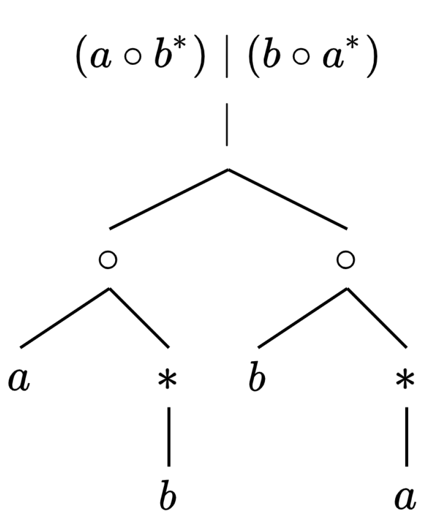
A regular expression p as defined in this paper is one of the following: the or operator ‘∣’ applied to two regular expressions and , the concatenation operator ‘∘’ applied to two regular expressions and , the star operator ‘’ applied to a regular expression , a symbol from the alphabet, the empty string, or the empty set. We call and subexpressions of p. We will not consider more advanced operators such as bracketed expressions that allow for a range of characters to be denoted within a few symbols, or captured groups that allow matched substrings to be recalled, or other added features that can make the problem NP-complete [23]. When considering the length of p, denoted , one can view this as the number of vertices in the parse tree for p, as seen in Figure 1. The precedence-setting braces in the regular expression do not contribute to its length as they do not appear as any vertex in the parse tree. To avoid confusion, we will always refer to the length of the text T as and the length of the pattern as , thereby reserving n for the matrices in Section 2. We will also always consider T as indexed from 1 to .
As mentioned in the introduction, this problem has to be solved frequently in applications. As such, different heuristics have been proposed [24,25]. Most of these heuristics use the idea of multi-grams. Multi-grams are small portions of text that will match some part of a substring in the inputted expression. In practice, applications often use multi-grams. Furthermore, to the author’s best knowledge, there are no solutions that preprocess the T and have a guaranteed time complexity less than that of any algorithmic solution. In the case where the pattern is given for preprocessing (rather than the text) work by Bille shows that after preprocessing time, each character in the text can be processed in time, where w is the word size [26].
For the algorithmic problem without any preprocessing, there exists a large body of research. The oldest and most fundamental solution is Thompson’s Method from 1968 [27]. This method locates substrings matching the regular expression p in time via the simulation of a nondeterministic finite automaton equivalent to p. Results by Myers improve this to time [28]. This was further improved to time in [29]. Additionally, a result by Bille and Thorup says that if p consists of k strings then the algorithmic problem can be solved in time [30]. In practice, for programming languages like Perl and Python, the simulation of this NFA is typically done using a method called back-tracking, which can lead to exponential time in the worst case. The main reason for this choice in implementation appears to be its simplicity [31].
To help answer why there have not been more significant advancements on the algorithmic problem, Backurs and Indyk established fine-grained lower bounds [13]. These lower bounds use the Strong Exponential Time Hypothesis (SETH). The proofs use a reduction from SETH to the problem of finding two orthogonal vectors, each from its own set (the Orthogonal Vectors problem). This is then reduced to pattern matching on regular expressions. The main idea in the final step is to use regular expressions to detect orthogonality between two vectors. The same technique is used in this paper in Section 2, although conditioned on a different conjecture. Both the work [13], as well as extensions of this work [32], focus on classifying regular expressions based on which types make pattern matching more difficult. We do not make such distinctions here.
2. Hardness of Creating an Index for Regular Expression Queries
The solution described in Section 3 requires exponential preprocessing and storage to see significant improvements in the query complexity over complete recomputation. In this section, we show that it is unlikely we will obtain a solution with polynomial preprocessing time and query time significantly better than , and even more unlikely we obtain one with query time significantly better than . All of the hardness results in this section hold for strings over an alphabet of size 3.
2.1. Hardness Based on OMv
The reduction here differs from the one in [13] in that the reduction here is from OMv (see Section 1 for a description of OMv) rather than the Orthogonal Vectors problem. This is done to add the notion of preprocessing. We adopt similar notation as was used there and consider this as the warm-up to the reduction used in Section 2.2.
Suppose the matrix M has the rows from top to bottom , …, where each is an binary vector. We set the text T as the concatenation of the corresponding binary strings using the character 2 as a delimiter, that is . Next we show how to process an input vector v into a regular expression p. The component gadget is the same as the one from [13]. It is
The definition is motivated by the fact that in the inner product of two vectors, 0 can be multiplied by either a 0 or 1 while maintaining that the inner product is 0. The definition is motivated by the fact that in the inner product of two vectors, 1 can only be multiplied by 0 while maintaining that the inner product is 0.
Next, we define the vector gadget as . Observe that our regular expression query pattern p has a length which is . For example, .
Lemma 1.
For , the pattern p matches a substring starting at index in T if and only if .
Proof.
First assume . If a component , we must have . By setting , we match this particular character. For all characters we set , thus all n characters in can be matched. This implies the substring for that starts at can be matched with .
To prove the converse, assume . Then there exists a component where and . Because , cannot be made to match the 1 character in T corresponding to . Additionally, because of the leading 2 symbols, this is the only character in the substring with which could be matched. The two observations combined imply the substring that starts at cannot be matched with p. □
Theorem 1.
For all , conditioned on the OMv conjecture, there does not exist an index that can answer regular expression queries in time, where is the size of the output. This holds even with arbitrary polynomial-time preprocessing.
Proof.
The OMv conjecture is that for an matrix M the OMv problem cannot be solved in time, even with polynomial preprocessing time. The input string T is of length , and we receive a total of n vectors that correspond to n regular expression queries. If each of the regular expression queries could be solved in for time (note that and the output size is at most ), then by Lemma 1 we can solve OMv in time , which is . □
It is natural to ask if we are not using the full power of our hypothetical solution for regular expression queries. After all, our solution can potentially report matching substrings starting at every index. In the above reduction, if we removed the 2s acting as delimiters, it would compute the orthogonality of the input vector v with every starting position in the linearized M. This can be used to compute the cross-correlation between two vectors with non-negative entries if one is only concerned with whether a resulting entry is zero or non-zero. By reversing one of the vectors, the convolution can also be computed. Specifically, we can modify our reduction to have T represent an binary vector and p the bottom-to-top reversal of a second binary vector (both padded with at least n zeros on either side). This allows us to compute the convolution .
By restricting the preprocessing time, we can obtain corollaries directly from the above reduction and the 3SUM hardness results established for the partial convolution indexing problem in [33]. Suppose along with the regular expression p we are given a set S of indices where we wish to know if a match starts. Call this the Partial Regular Expression Query problem. The following corollary is immediate from [33].
Corollary 1.
For all , conditioned on the 3SUM conjecture being true, there is no algorithm for the Partial Regular Expression Query problem with preprocessing time and query time, even if is .
2.2. Hardness Based on OMM
We will now utilize the OMM conjecture to strengthen our results. The reduction in this section requires only a single query pattern of size . This allows us to obtain a lower bound stronger than those obtained under OMv or 3SUM, but still conditioned on a plausible conjecture. See Section 1 for a description of the OMM conjecture.
Again, let , …, be the rows of the input matrix A that we can preprocess. We make . The substrings will allow us to deduce from each ending index of a match the vector used in the construction of p that is responsible for that match. As we will see, this is since a subexpression in p built from a vector has the suffix . Note that .
From the matrix B supplied at run time, we construct a regular expression p. Let B have the columns , …, from left to right. Using the same vector gadgets from Section 2.1, we set .
Lemma 2.
For there exists a substring matched by regular expression p starting in T at index and a substring matched ending at index iff where .
Proof.
First assume . This implies that . By the argument given in the proof for Lemma 1, this implies the subexpression matches the substring of T, which now starts at index . Moreover, we can match the subexpression of with the first j 1’s that follow in T, giving the final index of the match as .
To prove the converse, assume . This implies . By the argument given in Lemma 1, this implies that cannot be matched with . Furthermore, for any , if matches , then the final index of substring matching and starting at will be at , rather than . Hence, there can not be both a match starting at and a matching ending at . □
The output size of the query is bound by since each of the n subexpressions of p of form match T in at most n places. Because the output size does not exceed our desired lower bound we can apply Lemma 2 and the fact that to obtain Theorem 2.
Theorem 2.
For all , conditioned on the OMM conjecture, there does not exist an index that can answer regular expression queries in , where is the size of the output. This holds even with arbitrary polynomial-time preprocessing.
3. A Regular Expression Index
Before discussing our graph-based representations for query solutions we make a brief observation regarding the parse tree constructed from the regular expression. Within this rooted tree, each vertex represents the regular expression obtained by applying the operator labeling the vertex to the subexpressions represented by its children. The order in which these operators are applied is defined by the structure of the tree (see Figure 1). The leaves of the tree are either the empty string, the empty set, or symbols from the string’s alphabet. The ideas we present next are based on being able to quickly merge the solutions for each vertex of the tree.
3.1. Solution Graphs: Pattern Matching via Reachability
We take a slightly unorthodox view of regular expressions in this section. This viewpoint will make it easier to precompute solutions to small regular expression queries and then merge them with other solutions to answer the query. Essentially, we will view the solution for a regular expression query with regular expression p as a directed graph G where we are mainly concerned with the reachability from vertices in a set to vertices in another set . A solution graph for a given text T and regular expression p is defined as follows:
Definition 1
(Solution Graph). For a text T and regular expression p, a solution graph G is a directed graph that contains two distinguished sets of vertices and , called the start and end vertices, respectively. In G there exists a path from to a vertex if and only if the substring matches the regular expression p. Correspondingly, we will say that the regular expression given by the empty string matches the substring .
Solution graphs for a text and pattern are not unique. Moreover, there will typically be many additional vertices lying on the paths between the and , but we ultimately only care about the reachability between these two sets. Note also that this representation may require much more information than our final solution, which itself must only provide a list of starting positions and ending positions. We will demonstrate how these graphs can be merged together at every step while only using time for each vertex of the parse tree.
Merging Solution Graphs
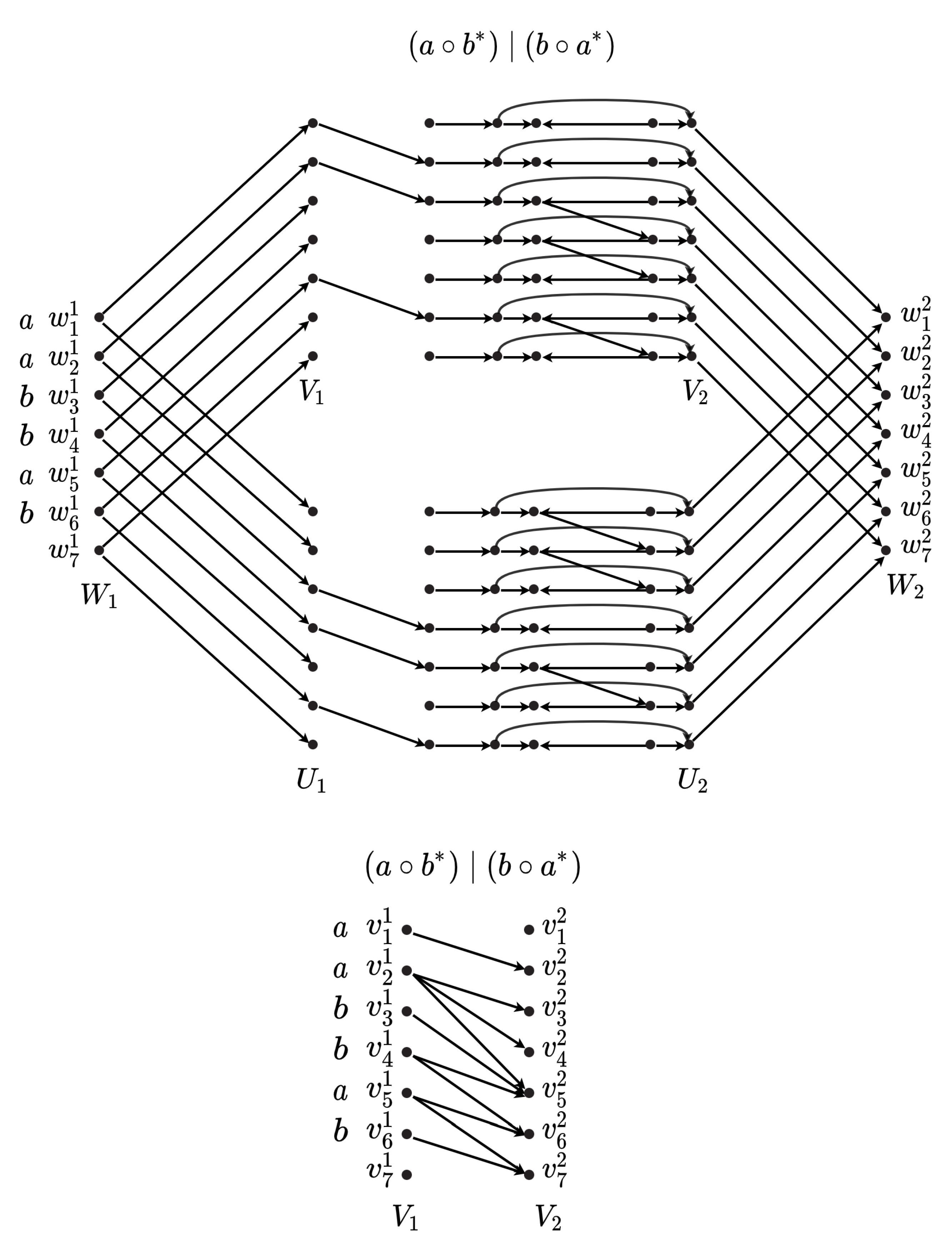
We now describe how solution graphs for subexpressions can be merged based on the operators used. We use this procedure both in the construction and in the query phase. It forms the key component of our technique. Illustrations are provided in Figure 2 and Figure 3. If the regular expression is only a single symbol, the solution graph is easily obtained as a bipartite graph, e.g., the top row of Figure 2.
First we consider the or operator ‘|’. Let be one regular expression with solution graph that has start and end vertex sets and . Let be a regular expression with solution graph that has start and end vertex sets and . To compute the graph G corresponding to , do the following:
- Graph G is initially equal to the two disconnected graphs and .
- Add two sets of new vertices and . These will be the new start and end vertex sets, respectively, of G.
- Add the directed edges: , , , and .
For the concatenation operator ‘∘’ we again take as the solution graph for pattern with start and end vertex sets and , respectively, and as the solution graph for pattern with start and end vertex sets and . To create the solution graph G for , do the following:
- Graph G is initially equal to the two disconnected graphs and .
- Make the start vertex set of G and the end vertex set of G.
- Add the directed edges: .
Lastly, we consider the star operator ‘*’ operator. Again taking , as the starting and ending vertex sets of for , construct the solution graph G for as follows:
- Graph G is initially equal to .
- Add two sets of new vertices and . These will be the start and end vertex sets, respectively, of G.
- Add the directed edges: , , , and .
In each step above edges are added to the resulting solution graph. Furthermore, any solution graphs that arise from matching a pattern consisting of only symbols (the leaves of the parse tree) have only edges. Therefore, a regular expression of length results in a solution graph having edges.
Lemma 3.
The constructions of G for theor(), concatenation(), andstar() operators result in G being a solution graph for the corresponding regular expression.
Proof.
The first two of these are straight forward, but we include them for completeness.
- (i)
- For the or operator, first consider when there exists a substring matched by . Then the substring must be matched by or . Say WLOG it is matched by , then there exists a path from to , which implies a path from to in G due to the edges and .
In the other direction, if there exists a path from to , it must start with either the edge or . Say WLOG it starts with the edge , then the final edge must be since there no edges between the graphs and . This implies a path through from to and hence the substring is matched by .
- (ii)
- For concatenation, first consider when there exists a substring matched by . Then there exists some k such that where is matched by and is matched by . Hence, there exists a path from to in and a path from to in . Connecting these paths using the edge we obtain the desired path.
In the other direction, if there exists a path from to then there must exist a path from to some and then a path from to , which implies is matched by and is matched by .
- (iii)
- For the star operator, Figure 2 is particularly helpfully in understanding the argument. We will use induction on x to show that all substrings matched by concatenations of correspond to a path from to . Suppose is matched by . If , then by the definition of , there exists a path from to . For , we assume our inductive hypothesis holds for all substrings of T matched by concatentations of . Since matches , there exists an index such that matches . Additionally, the substring is matched by . By our inductive hypothesis there exists a path from to and a path from to . Adding the connecting edge provides the path and proves that the induction holds.
To show that matching implies a path from to , if then (the empty string) is matched and the edge provides a path. If , then by the preceding paragraph we can use the edge , the path from to and the edge to obtain the desired path.
In the other direction, if there exists a path from to , and , then the corresponding substring is and so the substring is the empty string which is matched by . Otherwise , in which case the design of G implies there must be a path from to . Along this path any edges from to correspond to a substring of T matched by , and any edges from to correspond to the concatenation of two of these substrings. Putting these together we get that the substring is the concatenation of substrings matched by , and is therefore matched by . □
3.2. Precomputed Solutions
Having established how the solutions to sub-problems can be merged and pushed up to the root of our regular expression parse tree, we next describe how to use this fact to create solutions with the desired preprocessing/query time trade-off.
Solution Graphs for the Leaves. Each leaf represents either the empty set, the empty string, or an alphabet symbol. The empty set graph will have no edges, whereas the empty string has the edges for . For leaves with alphabet symbols, the solution graphs have the edges whenever matches the character labeling that leaf vertex.
Sampling Subtrees. We start with the observation that the number of vertices in the parse tree can be made linear in the number of leaves, despite vertices with the ‘’ label having only a single child. This is thanks to the property , which means that we can contract one of the star operator vertex if it appears as a child of another star operator vertex.
For a given value we can consider all regular expressions of length . With constant alphabet sizes, there are such regular expressions. For each of these, we will compute the solution graph for the root of its parse tree. For smaller patterns, this means that the solution graph for the whole parse tree will already be computed and the query response can be immediately given upon seeing the query. We store additional structures to deal with larger patterns. We store a bipartite graph that captures the reachability of start to end vertex sets in the solution graph and contains edges. An example of this can be seen in Figure 3. The bipartite graph is stored in the form of a Boolean adjacency matrix.
In more detail, suppose one has a bipartite graph G with vertex partitions and , each of size . Then given a subset S of vertices in , determining which vertices in are reachable from S can be done using the multiplication of a Boolean matrix M of size against a vector of size . The matrix M would have a 1 in entry iff is reachable from . The vector has a 1 for every entry in S and a 0 otherwise. The resulting product shows the reachable vertices in . The space required for storing all of these matrices is .
3.3. Constructing the Solution Graph at Query Time
A solution to a query is now a regular expression parse tree where every subtree of size or less has been replaced with a single vertex whose solution graph has been precomputed and is represented with a Boolean matrix. To obtain this final solution graph we proceed as described in the last section, recursively computing the solution until we obtain the graph at the root of the full parse tree. In doing so, we treat the precomputed solution graphs as merely a set of start and end vertices.
The total time to do this merging and obtain the final solution graph is . The precomputed solutions cut the number of leaves in the parse tree down by a factor of , and hence, by the observation that the number of internal vertices is linear in the number of leaves, it cuts the size of the parse tree down by a factor of as well. The parse tree now consists of vertex for non-precomputed solution graphs, each of which contributes edges when constructed, and Boolean matrices representing the reachability information of precomputed solution graphs. There are edges not represented by Boolean matrices.
3.4. Querying Matches via Graph Traversal
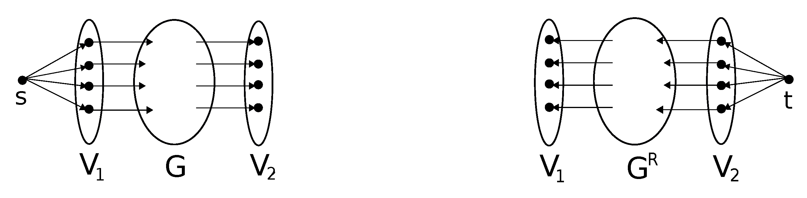
Adding an additional start vertex s and edges (see Figure 4), the query from s to detect reachability to the final set of ending vertices can be done by a graph traversal. During a traversal, when a subgraph represented by a Boolean matrix is arrived at, matrix multiplication can be performed (when beneficial) to more efficiently traverse the subgraph.
For general regular expressions, the star operator allows for the same subgraph to be visited multiple times. In the worst case, we return up to times to a subgraph where we may have the Boolean matrix representation. Rather than use the Boolean matrix multiplication, we take the adjacencies of each starting vertex. This results in a query time of . We reparameterize by setting . This makes the query time complexity and changes the space from to .
Theorem 3.
There exists a solution to answer existential regular expression queries with query time , requiring space and preprocessing time.
3.4.1. Restricted Regular Expressions
If we restrict ourselves to patterns with only concatenation and or operators (restricted regular expressions), using breadth-first-search all ‘start’ vertices of a subgraph are reached on the same level of the search. Hence for restricted regular expressions, we can better utilize the Boolean matrix representations of subgraphs, taking advantage of techniques developed for performing this multiplication more efficiently. Based on whether we desire a deterministic solution or a solution that is correct whp we obtain different space and preprocessing times.
Lemma 4
(Williams [34]). For all , every Boolean matrix A can be preprocessed in time such that every subsequent multiplication of A with an arbitrary Boolean n-vector x can be performed in time, on a pointer machine or a -word RAM.
Applying Lemma 4 with , the query time complexity becomes
We again reparameterize, setting . The query time becomes . The space complexity goes from to and the preprocessing time goes from to . The parameter ranges from 1 to .
Theorem 4.
For constant sized alphabets and some parameter fixed at construction, for patterns p containing only ‘concatenation’ and ‘or’ operators, there exists a data structure which answers regular expression existential queries in time requiring space and preprocessing time.
The techniques of Larson and Williams in [20] yield a randomized solution with better preprocessing time and space.
Lemma 5
([20]). With no preprocessing of the matrix and for any sequence of vectors , online matrix-vector multiplication of A and over the Boolean semiring can be performed in amortized time, with a randomized algorithm that succeeds whp.
Given a set of start vertices represented as a binary vector, this allows us to obtain the reachable end vertices using a randomized algorithm running in amortized time over queries that succeeds whp. For each matrix constructed, we apply multiplications against random binary vectors in preprocessing. The added time complexity of this operation is in total per matrix. This step is necessary to ensure the amortization techniques used in [20] will work.
The traversal is done in the same way as in the deterministic solution, only that each matrix-vector multiplication is repeated multiple times, and the most frequent of these solutions is taken as the output vector. We will show that under the conditions of for some , to maintain high probability of success of the overall algorithm it is sufficient to perform repetitions of each matrix multiplication. Therefore, each matrix during a query requires time. That yields an amortized query time of
where queries succeed whp. We reparameterize, setting .
Theorem 5.
Let T be a text over a constant sized alphabet and τ a parameter in fixed at construction. For patterns p containing onlyconcatenationandoroperators, where for , there exists a data structure which answers regular expression existential queries correctly whp in amortized time , requiring space and preprocessing time.
3.4.2. Preserving High Probability of Success
We know that our matrix-vector multiplication algorithm from [20] succeeds with probability for some . Our algorithm performs matrix-vector multiplication up to times. We assume the correctness of these matrix multiplications is independent. In the worst case, each of these has to be correct for our final answer to be correct. The probability that these are all correct is given by
Using the assumption that , this is bound below by . We will aim to preserve success whp by ‘amplifying’ to some . The technique we will use to do this is repeating each matrix multiplication a sufficient number (denoted by k) of times and using the most frequently resulting vector (the mode) as the solution.
Let be the random variable which is 1 if the multiplication on trial i is correct and 0 otherwise. Let be the probability with which the original matrix-vector multiplication algorithm is correct. The probability that the mode is correct is greater or equal to the probability that the correct solution is outputted at least times. We write the latter quantity as one minus the probability that the correct answer gets outputted less than half the time. Applying Chernoff bound, we get
Recall that we want our probability to be at least for some . Therefore we set the right-hand-side to and solve for to obtain
Since we want , it suffices then that we find the number of trials k such that
For we can easily bound q away from , making . Hence, repeating each matrix multiplication times and taking the mode provides the desired probability of success.
Obtaining Starting and Ending Positions. For each precomputed solution, we consider the edges reversed and the corresponding adjacency matrix as being precomputed. After constructing the final solution graph, we reverse all of its edges and add a single source vertex t and edges (see Figure 4). We call this graph . Using the same traversal techniques on as used on G yields the set of reachable starting vertices in .
4. Discussion
This work contributes to the growing number of fine-grained hardness results for string-related problems. The hardness results presented here belong to a narrower set of hardness results for indexing problems. We also provide here a solution to the indexing problem by utilizing recent innovations in Boolean matrix multiplication. Although requiring an exponential amount of space in terms of the length of the text, this solution allows for faster query times. A future research direction is to more elegantly incorporate the star operator into the above ideas, allowing for more space-efficient indexes that answer queries containing this operator.
Author Contributions
Both authors contributed equally to the concepts and proofs presented in this work. Both authors have read and agreed to the published version of the manuscript.
Funding
Supported in part by the U.S. National Science Foundation (NSF) under CCF-1703489.
Institutional Review Board Statement
Not applicable.
Informed Consent Statement
Not applicable.
Data Availability Statement
Not applicable.
Conflicts of Interest
The authors declare no conflict of interest.
References
- Banchs, R.E. Text Mining with MATLAB®; Springer Science & Business Media: Berlin/Heidelberg, Germany, 2012. [Google Scholar]
- Chapman, C.; Stolee, K.T. Exploring regular expression usage and context in Python. In Proceedings of the 25th International Symposium on Software Testing and Analysis (ISSTA 2016), Saarbrücken, Germany, 18–20 July 2016; pp. 282–293. [Google Scholar] [CrossRef]
- Donovan, A.A.; Kernighan, B.W. The Go Programming Language; Addison-Wesley Professional: Boston, MA, USA, 2015. [Google Scholar]
- Friedl, J.E.F. Mastering Regular Expressions—Understand Your Data and Be more Productive: For Perl, PHP, Java, .NET, Ruby; O’Reilly Media: Sebastopol, California, 2006. [Google Scholar]
- Goyvaerts, J.; Levithan, S. Regular Expressions Cookbook—Detailed Solutions in Eight Programming Languages, 2nd ed.; O’Reilly Media: Sebastopol, CA, USA, 2012. [Google Scholar]
- Karakoidas, V.; Spinellis, D. FIRE/J—Optimizing regular expression searches with generative programming. Softw. Pract. Exp. 2008, 38, 557–573. [Google Scholar] [CrossRef]
- Cox, R. Regular Expression Matching with a Trigram Index or How Google Code Search Worked. Available online: https://swtch.com/~rsc/regexp/regexp4.html (accessed on 3 March 2021).
- Devanbu, P.T. On “A Framework for Source Code Search Using Program Patterns”. IEEE Trans. Softw. Eng. 1995, 21, 1009–1010. [Google Scholar] [CrossRef]
- Umarji, M.; Sim, S.E. Archetypal Internet-Scale Source Code Searching. In Finding Source Code on the Web for Remix and Reuse; Springer: Boston, MA, USA, 2008. [Google Scholar]
- Chodorow, K.; Dirolf, M. MongoDB—The Definitive Guide: Powerful and Scalable Data Storage; O’Reilly Media: Sebastopol, CA, USA, 2010. [Google Scholar]
- Garofalakis, M.N.; Rastogi, R.; Shim, K. SPIRIT: Sequential Pattern Mining with Regular Expression Constraints. In Proceedings of the 25th International Conference on Very Large Data Bases (VLDB’99), Edinburgh, Scotland, UK, 7–10 September 1999; pp. 223–234. [Google Scholar]
- Obe, R.; Hsu, L. PostgreSQL—Up and Running: A Practical Guide to the Advanced Open Source Database; O’Reilly Media: Sebastopol, CA, USA, 2012. [Google Scholar]
- Backurs, A.; Indyk, P. Which Regular Expression Patterns Are Hard to Match? In Proceedings of the 2016 IEEE 57th Annual Symposium on Foundations of Computer Science (FOCS), New Brunswick, NJ, USA, 9–11 October 2016; pp. 457–466. [Google Scholar] [CrossRef] [Green Version]
- Henzinger, M.; Krinninger, S.; Nanongkai, D.; Saranurak, T. Unifying and Strengthening Hardness for Dynamic Problems via the Online Matrix-Vector Multiplication Conjecture. In Proceedings of the Forty-Seventh Annual ACM on Symposium on Theory of Computing (STOC 2015), Portland, OR, USA, 14–17 June 2015; pp. 21–30. [Google Scholar] [CrossRef] [Green Version]
- Abboud, A.; Dahlgaard, S. Popular Conjectures as a Barrier for Dynamic Planar Graph Algorithms. In Proceedings of the IEEE 57th Annual Symposium on Foundations of Computer Science (FOCS 2016), New Brunswick, NJ, USA, 9–11 October 2016; pp. 477–486. [Google Scholar] [CrossRef] [Green Version]
- Berkholz, C.; Keppeler, J.; Schweikardt, N. Answering Conjunctive Queries under Updates. In Proceedings of the 36th ACM SIGMOD-SIGACT-SIGAI Symposium on Principles of Database Systems (PODS 2017), Chicago, IL, USA, 14–19 May 2017; pp. 303–318. [Google Scholar] [CrossRef] [Green Version]
- Berkholz, C.; Keppeler, J.; Schweikardt, N. Answering UCQs under Updates and in the Presence of Integrity Constraints. In Proceedings of the 21st International Conference on Database Theory (ICDT 2018), Vienna, Austria, 26–29 March 2018; pp. 8:1–8:19. [Google Scholar] [CrossRef]
- Henzinger, M.; Neumann, S. Incremental and Fully Dynamic Subgraph Connectivity For Emergency Planning. In Proceedings of the 24th Annual European Symposium on Algorithms (ESA 2016), Aarhus, Denmark, 22–24 August 2016; pp. 48:1–48:11. [Google Scholar] [CrossRef]
- van den Brand, J.; Nanongkai, D.; Saranurak, T. Dynamic Matrix Inverse: Improved Algorithms and Matching Conditional Lower Bounds. In Proceedings of the 60th IEEE Annual Symposium on Foundations of Computer Science (FOCS 2019), Baltimore, MD, USA, 9–12 November 2019; pp. 456–480. [Google Scholar] [CrossRef] [Green Version]
- Larsen, K.G.; Williams, R.R. Faster Online Matrix-Vector Multiplication. In Proceedings of the Twenty-Eighth Annual ACM-SIAM Symposium on Discrete Algorithms (SODA 2017), Barcelona, Spain, 16–19 January 2017; pp. 2182–2189. [Google Scholar] [CrossRef] [Green Version]
- Blelloch, G.E.; Vassilevska, V.; Williams, R. A New Combinatorial Approach for Sparse Graph Problems. In Automata, Languages and Programming, Proceedings of the 35th International Colloquium (ICALP 2008), Reykjavik, Iceland, 7–11 July 2008; Part I: Tack A: Algorithms, Automata, Complexity, and Games; Springer: Berlin/Heidelberg, Germany, 2008; pp. 108–120. [Google Scholar] [CrossRef] [Green Version]
- Yuster, R.; Zwick, U. Fast sparse matrix multiplication. ACM Trans. Algorithms 2005, 1, 2–13. [Google Scholar] [CrossRef] [Green Version]
- Aho, A.V. Algorithms for Finding Patterns in Strings. In Handbook of Theoretical Computer Science, Volume A: Algorithms and Complexity; Elsevier: Amsterdam, The Netherlands, 1990; pp. 255–300. [Google Scholar]
- Tsang, D.; Chawla, S. An index for regular expression queries: Design and implementation. arXiv 2011, arXiv:1108.1228. [Google Scholar]
- Cho, J.; Rajagopalan, S. A Fast Regular Expression Indexing Engine. In Proceedings of the 18th International Conference on Data Engineering, San Jose, CA, USA, 26 February–1 March 2002; pp. 419–430. [Google Scholar] [CrossRef] [Green Version]
- Bille, P. New Algorithms for Regular Expression Matching. In Automata, Languages and Programming, Proceedings of the 33rd International Colloquium (ICALP 2006), Venice, Italy, 10–14 July 2006; Part I; Springer: Berlin/Heidelberg, Germany, 2006; pp. 643–654. [Google Scholar] [CrossRef] [Green Version]
- Thompson, K. Regular Expression Search Algorithm. Commun. ACM 1968, 11, 419–422. [Google Scholar] [CrossRef]
- Myers, E.W. A Four Russians Algorithm for Regular Expression Pattern Matching. J. ACM 1992, 39, 430–448. [Google Scholar] [CrossRef]
- Bille, P.; Thorup, M. Faster Regular Expression Matching. In Automata, Languages and Programming, Proceedings of the 36th International Colloquium (ICALP 2009), Rhodes, Greece, 5–12 July 2009; Part I; Springer: Berlin/Heidelberg, Germany, 2009; pp. 171–182. [Google Scholar] [CrossRef] [Green Version]
- Bille, P.; Thorup, M. Regular Expression Matching with Multi-Strings and Intervals. In Proceedings of the Twenty-First Annual ACM-SIAM Symposium on Discrete Algorithms (SODA 2010), Austin, TX, USA, 17–19 January 2010. [Google Scholar]
- Cox, R. Regular Expression Matching Can Be Simple and Fast (but Is Slow in java, perl, php, python, ruby,...). 2007. Available online: http://swtch.com/rsc/regexp/regexp1.html (accessed on 3 March 2021).
- Bringmann, K.; Grønlund, A.; Larsen, K.G. A Dichotomy for Regular Expression Membership Testing. In Proceedings of the 58th IEEE Annual Symposium on Foundations of Computer Science (FOCS 2017), Berkeley, CA, USA, 15–17 October 2017; pp. 307–318. [Google Scholar] [CrossRef] [Green Version]
- Goldstein, I.; Kopelowitz, T.; Lewenstein, M.; Porat, E. How Hard is it to Find (Honest) Witnesses? In Proceedings of the 24th Annual European Symposium on Algorithms (ESA 2016), Aarhus, Denmark, 22–24 August 2016; pp. 45:1–45:16. [Google Scholar] [CrossRef]
- Williams, R. Matrix-vector multiplication in sub-quadratic time: (Some preprocessing required). In Proceedings of the Eighteenth Annual ACM-SIAM Symposium on Discrete Algorithms (SODA 2007), New Orleans, LA, USA, 7–9 January 2007; pp. 995–1001. [Google Scholar]
Figure 1.
The parse tree for the regular expression .

Figure 2.
Solution graphs for the text . (Top): solution graphs for regular expressions a and b. Second from top: solution graphs for the regular expressions and . Second from the bottom: solution graph for . (Bottom): solution graph for .
Figure 2.
Solution graphs for the text . (Top): solution graphs for regular expressions a and b. Second from top: solution graphs for the regular expressions and . Second from the bottom: solution graph for . (Bottom): solution graph for .

Figure 3.
Solution graphs for the text . (Top): the solution graph for . (Bottom): an equivalent, simpler solution graph for .
Figure 3.
Solution graphs for the text . (Top): the solution graph for . (Bottom): an equivalent, simpler solution graph for .

Figure 4.
On the (left), we have the querying strategy to find all ending vertices corresponding to pattern matches. On the (right), we reverse the edges in G to form . The graph can be used to find starting vertices that correspond to the starting indices of pattern matches.
Figure 4.
On the (left), we have the querying strategy to find all ending vertices corresponding to pattern matches. On the (right), we reverse the edges in G to form . The graph can be used to find starting vertices that correspond to the starting indices of pattern matches.

Publisher’s Note: MDPI stays neutral with regard to jurisdictional claims in published maps and institutional affiliations. |
© 2021 by the authors. Licensee MDPI, Basel, Switzerland. This article is an open access article distributed under the terms and conditions of the Creative Commons Attribution (CC BY) license (https://creativecommons.org/licenses/by/4.0/).
Share and Cite
MDPI and ACS Style
Gibney, D.; Thankachan, S.V. Text Indexing for Regular Expression Matching. Algorithms 2021, 14, 133. https://0-doi-org.brum.beds.ac.uk/10.3390/a14050133
AMA Style
Gibney D, Thankachan SV. Text Indexing for Regular Expression Matching. Algorithms. 2021; 14(5):133. https://0-doi-org.brum.beds.ac.uk/10.3390/a14050133
Chicago/Turabian StyleGibney, Daniel, and Sharma V. Thankachan. 2021. "Text Indexing for Regular Expression Matching" Algorithms 14, no. 5: 133. https://0-doi-org.brum.beds.ac.uk/10.3390/a14050133
Note that from the first issue of 2016, this journal uses article numbers instead of page numbers. See further details here.